Dynamic optimization of open-pit coal mine production scheduling based on ARIMA and fuzzy structured element

A dynamic optimization method was created to address the production schedule issue in an open-pit coal mine while taking into account the characteristics of the fuzzy structured element. The fuzzy mining capacities of all “geologically optimal push-back bodies” were then examined using the moving cove method. One of the most crucial elements in the process of open-pit coal mine production scheduling optimization is coal pricing. As a result, this work also presents a dynamic optimization technique for production scheduling that incorporates the prediction of economic time series and the generation of dynamic economic indices. An appropriate time series model is created to forecast the future coal price based on previous data on coal prices. The prediction results are used in the calculation of optimal mining body generation to dynamically obtain the optimal production scheduling model. The Baorixile Open-pit Coal Mine in China’s Inner Mongolia Autonomous Region is using this method. The Autoregressive Integrated Moving Average Model ARIMA is constructed to anticipate the coal price in the future 23 years by evaluating and processing the coal price from 2009 to 2022, and the ideal production scheduling scheme of the mine economics is afterwards identified. The ideal fuzzy coal mining volume, the potential production life, and the fuzzy total net present value (NPV) of the annual production scheduling are all provided at the same time. The optimization findings can better give fundamental support for mine design and future production since the fuzzy problem is accurately expressed by correct formulations.

1 Introduction

A prominent place is held by open-pit coal mines in the worldwide coal industry. The share of open-pit coal mining in major coal-mining nations like the United States, Australia, Russia, and India is more than 50%, and some countries reach more than 90% (He et al., 2006; Zheng et al., 2014; Wang et al., 2022). The main objective of the OPCMPS is to choose a coal and waste rock extraction sequence that is technically viable and has the greatest possible total economic advantages. The term “technically feasible” refers to the OPCMPS having to adhere to a number of technical requirements; to maximize the entire NPV realized by deposit mining is to obtain the “greatest possible total economic advantages” (Ramazan, 2007; Osanloo et al., 2008; Khan and Niemann-Delius, 2018; Gilani et al., 2020; Fathollahzadeh et al., 2021). Saving non-renewable resources, safeguarding the ecosystem on which people depend for existence, and enhancing total economic gains throughout the mining life cycle are all greatly aided by the OPCMPS in the mine design (Nelson and Goldstern, 1980; Fytas, 1986; Chicoisne et al., 2012; Alipour et al., 2020). Therefore, the optimization design of OPCMPS has been extensively researched since the 1980s and 1990s (Caccetta and Hill, 2003; Bienstock and Zuckerberg, 2009; Boland et al., 2009).

The production scheduling issue has been the subject of much study effort by many professionals and academics. For short-term production scheduling: A multidestination mixed integer linear programming model for short-term open pit mine production scheduling was proposed by Eivazy and Askari-Nasab (2012). The model takes into consideration choices regarding buffer and blending stocks, horizontally directed mining, and ramps. It decreases the whole cost of mining operations, including extraction, processing, transporting, rehandling, and rehabilitation. The following items were presented by Blom et al. (2017): A tool for constructing multiple, diverse, short-term schedules that meet a variety of common objectives without the need for iterative parameter adjustment; and a novel concurrent rolling horizon-based algorithm for the generation of multiple distinct production schedules, each optimized concerning a series of objectives. Using hierarchical decomposition (HDP), Blom et al. (2018) introduced a unique hierarchical decomposition-based approach (HDP). It also provides an experimental comparison of this technique with a scheduling approach based on receding horizon controls. HDP may be used to solve any scheduling issue, not only those that arise in the mining industry. Upadhyay and Askari-Nasab (2018) provide a simulation-optimization framework/tool to take into account uncertainty in mining operations for reliable short-term production planning and proactive decision making. With the use of a goal programming-based mine operational optimization tool and a discrete event simulation model of mine operations, this framework/tool creates a short-term schedule based on uncertainty. For long-term production scheduling: Tolouei et al. (2021a) presented hybrid models to elucidate the long-term production scheduling problem regarding grade uncertainty, and the results show that the models generate a near-optimal solution within a reasonable time. The same year, due to the deterministic assumption and grade uncertainty, Tolouei et al. (2021b) proposed hybrid models that combine the Lagrangian relaxation (LR) approach with meta-heuristic techniques, the bat algorithm, and particle swarm optimization to solve the LTPSP. Utilizing meta-heuristic techniques, the Lagrange multipliers have been updated. The results from the case studies show that, in comparison to other strategies, the LR-bat algorithm hybrid approach may provide a solution that is near to optimum in terms of cumulative NPV, average ore grade, and computing time during a 12-years production period. Khan (2018) uses two distinct computationally effective population-based metaheuristic techniques, based on particle swarm optimization (PSO) and the bat algorithm, to solve one specific stochastic variant of the open pit mine scheduling problem, i.e., the two stage stochastic programming model with recourse for figuring out the long-term production schedule of an open pit mine under the condition of grade uncertainty. Turan and Onur (2022) improved cone extraction sequencing to ascertain the ultimate pit limit. Following that, a long-term production schedule was created utilizing the modified floating cone method’s cone extraction approach and parametric analysis strategy. This method allows for the mining of ore blocks with the same annual production quantity throughout the course of each cycle.

Almost all of the above studies take metal open-pit mines as the research object. It can be found that a large number of researchers have focused their attention on the optimization of production scheduling in open-pit metal mines, but rarely on the optimization of production scheduling in open-pit coal mines. Therefore, Gu et al. (2011) proposed a dynamic sorting method for open-pit coal mines to simultaneously optimize the final pit and production scheduling of mines. The method can simultaneously solve the optimal final pit, mine life, annual recoverable amount of waste rock and coal, and mining sequence. Its flexibility is that it can easily incorporate constraints such as maximum strip ratio, maximum and minimum mining capacity. However, the preparation of an open-pit coal mine production plan should take into account the number of equipment, the number of personnel, the width of the security platform, and the production capacity of available equipment; the maximization of overall economic benefits should be based on the perspective of dynamic economics to maximize the total NPV. In actual production, due to the influence of equipment failure, inaccurate geological model caused by insufficient geological exploration, landslide of working slope, weather and other factors, the actual annual coal mining volume and stripping volume are uncertain and fuzzy, which will lead to the total NPV is also fuzzy. In the process of calculating the NPV, the coal price is often calculated with the average value of coal price in recent years, without considering the variability of coal price. How to solve the reliability of economic parameters is also the key issue in the dynamic optimization of production scheduling. Therefore, based on the research of literature (Gu et al., 2011), this study proposes a dynamic optimization method of mine production scheduling based on fuzzy mining quantity and fuzzy stripping quantity of production plan determined by economic time series prediction production cost and coal sales price combined with the fuzzy structural element. The dynamic optimization of production scheduling considering economic variability and fuzzy stripping quantity is realized, and the fuzzy interval of maximum NPV is obtained. At the same time, the possibility of each value in the interval is given. The effectiveness of the method is verified by an example.

The following sections present the framework and application of the approach. Section 2 introduces the principle of fuzzy structure element; Section 3 explains the dynamic optimization method of geologically optimal mining limit and production scheduling described in the literature (Gu et al., 2011); Section 4 describes the principle of the price time series prediction method; Section 5 contains all the details and processes of the proposed method; To demonstrate the viability of the dynamic optimization approach suggested in this work, a real mine is used in Section 6; Section 7 presents the contribution of this paper to the research field and the characterization of the proposed method, and discusses the experimental results; And, finally, the conclusions are presented in Section 8.

2 Related theory of the fuzzy structured element

In 2002, Guo Sicong presented the fuzzy structure element analysis approach as a solution to the metadata fuzzy operation issue (GUO, 2002a; GUO, 2002b; GUO, 2009; Guo and Song, 2011). This article introduces the fuzzy structured element to achieve OPCMPS dynamic optimization. The basic concept, theorem, and properties of the fuzzy structured element are briefly introduced in this section.

2.1 Fuzzy structured element of the fuzzy number

2.1.1 Definition 1

Let $E$ is a fuzzy set on the real number field $R$, and $E\left(x\right)$ represents the membership function of E, and $x\in R$. Then, $E$ is called a fuzzy structured element on $R$, if

• $E\left(x\right)=1$.

• $E\left(x\right)$ is a function of monotone increasing and right continuous on [(−1, 0), monotone decreasing and left continuous on (0, 1)].

• $E\left(x\right)=0$, When $\mathrm{x}\in \left(-\infty ,-1\right)$ or $\mathrm{x}\in \left(1,+\infty \right)$.

For example, $E$ also is known as a triangle structured element, The graph membership function is shown in Figure 1A, if $E$ has a membership function:

$E\left(x\right)=\{\begin{array}{cc}1+x,& -1\le x\le 0\\ 1-x,& 0\le x\le 1\\ 0,& \mathrm{o}\mathrm{t}\mathrm{h}\mathrm{e}\mathrm{r}\mathrm{w}\mathrm{i}\mathrm{s}\mathrm{e}\end{array}(1)$

FIGURE 1

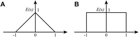
FIGURE 1. Fuzzy structured element. (A) Triangle structured element; (B)Rectangle structured element.

Then $E$ also known as a rectangle structured element, the graph membership function is shown in Figure 1B, if $E$ has a membership function:

$E\left(x\right)=\{\begin{array}{cc}1,& -1\le x\le 1\\ 0,& \mathrm{o}\mathrm{t}\mathrm{h}\mathrm{e}\mathrm{r}\mathrm{w}\mathrm{i}\mathrm{s}\mathrm{e}\end{array}(2)$

2.1.2 Definition 2

E is called a canonical fuzzy structural element, if E satisfies the following conditions:

• $\forall x\in \left(-1,1\right)$, $E\left(x\right)>0$.

• $E\left(x\right)$ is a function of strictly increasing monotonically and continuous on [(−1, 0), strictly decreasing monotonically and continuous on (0, 1)].

Then, E is called a symmetric fuzzy structural element. if $E\left(x\right)=E\left(-x\right)$.

2.1.3 Theorem 1

Let E be a fuzzy structured element and $E\left(x\right)$ is its membership function, the function $f\left(x\right)$ is continuous and monotone on [−1,1], then $f\left(E\right)$ is a fuzzy number, and the membership function of $f\left(E\right)$ is $E\left(f^{-1}\left(x\right)\right)$, (where $f^{-1}\left(x\right)$ is rotational symmetry function for variable x and y, if f is a strictly monotone function, then $f^{-1}\left(x\right)$ is the inverse function of $f\left(x\right)$).

2.1.4 Theorem 2

For a given canonical fuzzy structured element E and any finite fuzzy number $\underset{\sim }{A}$, there always exists a monotone bounded function $f\left(x\right)$ on [−1,1], having the form $A=f\left(E\right)$, and $u_{\underset{\sim }{A}}\left(x\right)=E\left(f^{-1}\left(x\right)\right)$.

2.1.5 Character 1

Let $\underset{\sim }{A}$ and $\underset{\sim }{B}$ are fuzzy numbers generated linearly by the fuzzy structure element E. Let $\underset{\sim }{A}=a+\alpha E$, $\underset{\sim }{B}=b+\beta E$, then, $\underset{\sim }{A}+\underset{\sim }{B}=\left(a+b\right)+\left(\alpha +\beta \right)E=c+\gamma E$, $u_{\underset{\sim }{A}+\underset{\sim }{B}}\left(x\right)=E\left(\frac{x-c}{\gamma }\right)=E\left(\frac{x-\left(a+b\right)}{\alpha +\beta }\right)$; $k\underset{\sim }{A}=ka+k\alpha E$; $u_{k\underset{\sim }{A}}\left(x\right)=E\left(\frac{x-ka}{ka}\right)$

2.2 Fuzzy numbers structured element weighted order

2.2.1 Definition 3

Let $\underset{\sim }{A},\underset{\sim }{B}\in {\underset{\sim }{N}}_c\left(R\right)$, $\underset{\sim }{A}=f\left(E\right)$, $\underset{\sim }{B}=g\left(E\right)$, E is a canonical fuzzy structure element, $E\left(x\right)$ is a membership function. $f$ and $g$ are the same ordered monotonic functions of membership on [−1, 1]. Then the relation “≤” determined by Eq. 3 is the fuzzy numbers structured element weighted order.

$\underset{\sim }{A}\le \underset{\sim }{B}\iff F\left(\underset{\sim }{A},\underset{\sim }{B}\right)={\int }_{-1}^{1}E\left(x\right)\left(f\left(x\right)-g\left(x\right)\right)dx\le 0(3)$

Let $\underset{\sim }{A}$ is a triangular fuzzy number, $\underset{\sim }{A}=\left(a;a^{-},a^{+}\right)$ for short, if the membership function of the fuzzy number $\underset{\sim }{A}$ is:

$E\left(x\right)=\{\begin{array}{cc}\frac{x-a+a^{-}}{a^{-}},& a-a^{-}\le x\le a\\ \frac{a+a^{+}-x}{a^{+}},& a\le x\le a+a^{+}\\ 0& \mathrm{o}\mathrm{t}\mathrm{h}\mathrm{e}\mathrm{r}\mathrm{w}\mathrm{i}\mathrm{s}\mathrm{e}\end{array}(4)$

2.2.2 Theorem 3

If $\underset{\sim }{A}=\left(a;a^{-},a^{+}\right)$ and $\underset{\sim }{B}=\left(b;b^{-},b^{+}\right)$ are fuzzy numbers, then E is the triangular fuzzy structural element, then:

$\underset{\sim }{A}\le \underset{\sim }{B}\iff a+\frac{a^{+}-a^{-}}{6}\le b+\frac{b^{+}-b^{-}}{6}(5)$

The proof of the above theorems can be found in References (Caccetta and Hill, 2003; Bienstock and Zuckerberg, 2009; Boland et al., 2009; Eivazy and Askari-Nasab, 2012).

3 Geologically optimum final pits and their dynamic programming

The highest coal amount among all final pits with volume V in the mining region where the working slope angle does not exceed β is referred to as the geologically optimum final pit. The final pit optimization of OPCMPS is based on the pre-designed annual total mining volume (the sum of the coal mining volume and the stripping volume), and it is based on the corresponding mining parameters to determine the optimal state of the end of every year, which is the state of maximum coal volume in the same mining volume. So it is also possible to achieve the ideal coal mining and stripping volumes. There are multiple states in the mining areas that meet the annual mining volume. It is naturally known that the maximum coal mining volume in the total mining volume that meets the requirements should be the optimization, that is, the OPCMPS that meets the technical feasibility and the maximum total NPV should be found from a series of geological optimum mining pits, and the total NPV is related to the coal mining volume, stripping volume and mining cost.

Therefore, according to the thought of the Reference (Gu et al., 2011), it is assumed that M geological optimum mining pits are obtained in final pits, i.e., ${\left\{p\right\}}_{\mathrm{m}}=\left\{p_1,p_2,\dots ,p_{\mathrm{m}}\right\}$, where p₁ is the smallest pit and p_m is the largest pit, each element in the sequence may be the optimum one. As shown in Figure 2.

• Stage decision variables: in the state p_i, the coal volume is q_i and the stripping volume is w_i.

• State variables: $s\left(t,i\right)$ represents the i state of the t stage, corresponding to the kth mining body of ${\left\{p\right\}}_{\mathrm{m}}$. S (t-1, i) represents the j state of the t-1 stage, corresponding to the kth mining body of ${\left\{p\right\}}_{\mathrm{m}}$.

• State transition equation: let the coal content of the first k mining bodies be q_k and the stripping amount be w_i.

• Objective function: the state transfer profit of each stage is:

$G_{\left(t,i\right)}^{\left(t-1,j\right)}=\left(p_t-c_t\right)q_{\left(t,i\right)}^{\left(t-1,j\right)}-b_t{w}_{\left(t,i\right)}^{\left(t-1,j\right)}-z_t\left(q_{\left(t,i\right)}^{\left(t-1,j\right)}+w_{\left(t,i\right)}^{\left(t-1,j\right)}\right)(6)$

Where $p_{\mathrm{t}}$ is the unit coal price in stage t, $c_{\mathrm{t}}$ is the unit coal mining cost in stage t, $b_{\mathrm{t}}$ is the unit stripping cost in stage t.

FIGURE 2

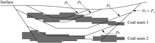
FIGURE 2. Push-backs in a final pit.

NPV refers to the sum of the annual net cash flow by the industry to the base year present value at the beginning of the calculation period in the economic or physical life cycle of the project. When NPV ≥ 0, the project is feasible, and when NPV ≤ 0, the project is not feasible. NPV is a relatively scientific evaluation method of investment scheme. After the time attribute of the ore block and the ore price at corresponding time points are known, the NPV of the boundary scheme can be calculated according to the concept of NPV. According to economic theory, the total NPV should be used as the standard to evaluate the subsequence profit of mining bodies. In view of this, let the maximum NPV from state 0 to state $s\left(t-1,j\right)$ be $NP{V}_{\left(t-1,j\right)}$, and transfer to state $s\left(t,i\right)$ be $NP{V}_{\left(t,j\right)}$, then:

$NP{V}_{\left(t,i\right)}=\underset{j\in J\left(t,i\right)}{\max }\left\{NP{V}_{\left(t-1,j\right)}+\frac{G_{\left(t,i\right)}^{\left(t-1.j\right)}}{{\left(1+d\right)}^t}\right\}(7)$

Where $J\left(t,i\right)$ is the decision set, which represents a state set of state $s\left(t,i\right)$ that may be transferred from stage t-1 to the next stage.

4 Price time series prediction method

Given the dominant position of coal in China’s energy market, fluctuating coal prices not only determine the survival of coal enterprises but also directly affects economic growth, energy security and industrial raw material supply (Li and Lin, 2017; Jiang et al., 2018; Wang et al., 2020; Zhang et al., 2020; Liu, 2021). Therefore, this paper combines economic time series with production scheduling optimization for the first time. Oskar Morgenstern, German Realmist (Clements and Hendry, 1998), first systematically discussed the method of economic forecasting in 1928. Box et al. (2015) proposed the famous Auto-Regressive Moving Average (ARMA) model in 1976, and then Harvey (1990) and Hendry and Doornik (1994) improved it. Auto-Regressive Integrated Moving Average (ARIMA) model is a well-known statistical technique for predicting time series. Numerous studies have demonstrated that the ARIMA model is effective in predicting outcomes in linear time series analysis with high levels of accuracy (Contreras et al., 2003; Li, 2021). Its benefits include a straightforward model and the absence of any additional exogenous variables. There are certain restrictions, though. For example, the time series data must be steady or stable after differential differentiation. In essence, it only detects linear correlations and ignores nonlinear ones. Comparing the ARIMA model to approaches like machine learning, its simplicity may assure the efficiency in the dynamic optimization process of open-pit coal mine production scheduling. The ARIMA model’s forecast accuracy matches the necessary forecasting criteria. The model can be expressed as ARIMA (p, d, q), where p is the autoregressive order, d is the different order, and q is the moving average order. When d = 0, the model can be expressed as ARMA (p, q), namely the autoregressive moving average model; but when p, d, and q are not equal to 0, the model is expressed as ARIMA (p, d, and q), that is, the autoregressive summation moving average model. ARIMA (p, q) model refers to the linear function that the time series can be expressed as the current and previous random error term and the previous value, and its expression is shown in Eq. 8, where $y_t$ is the time series; $\theta$ is the moving average coefficient; $\phi$ is a self-regression coefficient; $u_t$ is an independent white noise sequence, and obeys the normal distribution with a mean value of 0 and variance of ${\sigma }_u^2$.

$y_t={\phi }_1{y}_{t-1}+{\phi }_2{y}_{t-2}+\cdots +{\phi }_p{y}_{t-p}+u_t-\left({\theta }_1{u}_{t-1}+{\theta }_2{u}_{t-2}+\cdots +{\theta }_p{u}_{t-p}\right)(8)$

ARIMA (p, d, q) is a random sequence model with a d-order difference of time series, its expression is shown in Eq. 9, where $B^k$ is a delay operator and can be expressed as $y_{t-k}/y_t$.

$y_t=\frac{\left(1-{\theta }_{1}B-{\theta }_2{B}^2-\dots -{\theta }_q{B}^q\right)u_t}{1-{\phi }_{1}B-{\phi }_2{B}^2-\dots -{\phi }_p{B}^p}(9)$

Time series prediction analysis mainly includes the following steps:

Step-1. Sequence autocorrelation and partial correlation analysisThe simple correlation between each sequence value that constitutes a time series is called autocorrelation, and the autocorrelation coefficient r_k is calculated by Eq. 10, where n is the sample size, k is the lag period, and $\overline{y}$ is the arithmetic mean of the sample data.

$r_k=\frac{{\displaystyle \sum }_{j=1}^{n-k}\left(y_1-\overline{y}\right)\left(y_{t+k}-\overline{y}\right)}{{\displaystyle \sum }_{j=1}^n{\left(y_t-\overline{y}\right)}^2}(10)$

Partial autocorrelation refers to the conditional correlation between $y_t$ and $y_{t-k}$ under the given conditions of $y_{t-1},y_{t-2},\dots ,y_{t-k+1}$ for time series $y_t$. The partial autocorrelation coefficient is calculated by Eq. 11. When k=1, a=b.

${\phi }_{kk}=\frac{r_k-{\displaystyle \sum }_{j=1}^{k-1}{\phi }_{k-1,j}{r}_{k-j}}{1-{\displaystyle \sum }_{j=1}^{k-1}{\phi }_{k-1,j}{r}_j}(11)$

The autocorrelation and partial autocorrelation of sequences are an important basis for judging the stability of sequences and selecting the type and order of prediction models.

Step-2. Model-based parameter estimationThe commonly used model parameter estimation methods include Yule-Walker correlation moment estimation, least-squares estimation, maximum likelihood estimation and entropy estimation methods. The first method is mainly for the AR model, and the second method is generally for the MA model. The mixture of the two methods can be used for the ARMA model.

Step-3. Predictive analysisTime series prediction refers to the prediction of future $y_{t+l}\left(l>0\right)$ in $t+l$ period if $y_t$ is known. Since the time t is known, the predicted value of $y_{t+l}$ can be called the first step prediction starting from the time t. It is stated that to obtain the best prediction effect, the mean square error between the predicted value and the true value $y_{t+l}$ is required to be minimized, that is, to minimize $E{\left[y_{t+l}-{\widehat{y}}_l\right]}^2$. The predicted minimum variance is obtained from the conditional expectation of $y_{t+l}$, that is, ${\widehat{y}}_l\left(l\right)=E\left(y_{t+l}|y_t,y_{t-1},\cdots \cdots \right)$. Therefore, as long as the model of $y_t$ is established, ${\widehat{y}}_l\left(l\right)$ can be derived. The reversal form of ARMA prediction is shown in Eq. 12, that is, the predicted value ${\widehat{y}}_l\left(l\right)$ is the linear combination of all the data at present and in the past, and the coefficient $w_j$ is determined by the inverse function.

${\widehat{y}}_t\left(l\right)={\displaystyle \sum }_{j=1}^{\infty }{w}_j{y}_{t+1-j}(12)$

5 Dynamic sequencing of geological optimum final pit based on structure element theory

Annual actual coal mining and stripping values tend to fluctuate around planned values because they have uncertainty in production. Therefore, the maximum total net present value OPCMPS should be made in the final mining pit, and the annual coal mining and stripping should be regarded as fuzzy numbers. Since the fuzzy number represented by the fuzzy structured element can avoid the complex traversal problem based on the traditional expansion principle in the operation process, the fuzzy structured elements are used to represent the fuzzy coal mining volume and the fuzzy stripping volume.

Let ${\underset{\sim }{q}}_i$ is the fuzzy coal mining volume in state $i$, ${\underset{\sim }{w}}_i$ is the fuzzy stripping volume in state i, and they are linearly generated by symmetric fuzzy structured elements. Let ${\underset{\sim }{q}}_i=a_i+b_{i}E,{\underset{\sim }{w}}_i=c_i+d_{i}E$, then $f\left(x\right)$ and $g\left(x\right)$, two same ordered monotonic functions, can be found on [−1, 1] through Theorem 1. Let $f_i\left(x\right)=a_i+b_{i}x,g_i\left(x\right)=c_i+d_{i}x$, ${\underset{\sim }{q}}_i=f_i\left(E\right)$ and ${\underset{\sim }{w}}_i=g_i\left(E\right)$. So, in the process of state transferred of state $s\left(t-1,j\right)$ to $s\left(t,j\right)$ from stage t-1to stage t, the analytic expression of each index generated by the liner structured element is as follows:

(1) The fuzzy coal mining volume is:

${\underset{\sim }{q}}_{\left(t,i\right)}^{\left(t-1,j\right)}={\underset{\sim }{q}}_k-{\underset{\sim }{q}}_n=f_k\left(E\right)-f_n\left(E\right)=\left(a_k-a_n\right)+\left(b_k-b_n\right)E(13)$

Its membership function is:

$u_{{\underset{\sim }{q}}_{\left(t,i\right)}^{\left(t-1,j\right)}}\left(x\right)=E\left({\left(f_k+f_n^{\tau 1}\right)}^{-1}\left(E\right)\right)=E\left(\frac{x+a_n-a_k}{b_k+b_n}\right)(14)$

(2) The fuzzy stripping volume is:

${\underset{\sim }{w}}_{\left(t,i\right)}^{\left(t-1,j\right)}={\underset{\sim }{w}}_k-{\underset{\sim }{w}}_n=g_k\left(E\right)-g_n\left(E\right)=\left(c_k-c_n\right)+\left(d_k+d_n\right)E(15)$

Its membership function is:

$u_{{\underset{\sim }{q}}_{\left(t,i\right)}^{\left(t-1,j\right)}}\left(x\right)=E\left({\left(g_k+g_n^{\tau 2}\right)}^{-1}\left(E\right)\right)=E\left(\frac{x+c_n-c_k}{d_k+d_n}\right)(16)$

(3) The fuzzy state transferred profit is:

$\begin{array}{l}{\underset{\sim }{G}}_{\left(t,i\right)}^{\left(t-1,j\right)}=p_t{\underset{\sim }{q}}_{\left(t,i\right)}^{\left(t-1,j\right)}-c_t{\underset{\sim }{q}}_{\left(t,i\right)}^{\left(t-1,j\right)}-b_t{\underset{\sim }{w}}_{\left(t,i\right)}^{\left(t-1,j\right)}-z_t\left({\underset{\sim }{q}}_{\left(t,i\right)}^{\left(t-1,j\right)}+{\underset{\sim }{w}}_{\left(t,i\right)}^{\left(t-1,j\right)}\right)\\ =\left(p_t-c_t-z_t\right)\left[\left(a_k-a_n\right)+\left(b_k+b_n\right)E\right]-\left(b_t+z_t\right)\left[\left(c_k-c_n\right)+\left(d_k+d_n\right)E\right]\end{array}(17)$

Its membership function is:

$\begin{array}{l}{u}_{{\underset{\sim }{G}}_{\left(t,i\right)}^{\left(t-1,j\right)}}\left(x\right)=E\left(\left(\left(p_t+c_t+z_t\right){\left(f_k-f_n^{{\tau }_1}\right)}^{-1}\left(E\right)\right)+\left(b_t+z_t\right)\left({\left(g_k+g_n^{{\tau }_2}\right)}^{-1}\left(E\right)\right)\right)\\ =E\left(\frac{x+\left(c_t+z_t-p_t\right)\left(a_k-a_n\right)+\left(b_t+z_t\right)\left(c_k+c_n\right)}{\left(p_t+c_t+z_t\right)\left(b_k+b_n\right)+\left(b_t+z_t\right)\left(d_k+d_n\right)}\right)\end{array}(18)$

(4) Accordingly, the fuzzy NPV transferred to the state $s\left(t,i\right)$ is:

$N\underset{\sim }{P}{V}_{\left(t,i\right)}=\underset{j\in J_{\left(t,i\right)}}{\max }\left\{N\underset{\sim }{P}{V}_{\left(t-1,j\right)}+\frac{{\underset{\sim }{G}}_{\left(t,i\right)}^{\left(t-1,j\right)}}{{\left(1+d\right)}^t}\right\}(19)$

Its membership function is:

$u_{N\underset{\sim }{P}{V}_{\left(t,i\right)}}\left(x\right)=\underset{j\in J_{\left(t,i\right)}}{\max }\left\{u_{N\underset{\sim }{P}{V}_{\left(t-1,j\right)}}\left(x\right)+\frac{u_{{\underset{\sim }{G}}_{\left(t,i\right)}^{\left(t-1,j\right)}}\left(x\right)}{{\left(1+d\right)}^t}\right\}(20)$

To explain the solving process of the model, take Figure 2 as an example for a brief illustration. It can be seen from Figure 2 that 5 geologically optimum pits are produced in the final mining pit, and the possible state transferred mode is shown in Figure 3 (In the actual calculation, tens or hundreds or even more optimum mining pits will be produced. Therefore, a state transferred mode should be drawn base on the actual situation.). Suppose that a sequence of 5 geologically optimum push-backs within a geologically optimum pit F_i has been generated as shown by p₁ to p₅ in Figure 2. A dynamic programming scheme is set up as shown in Figure 3. The horizontal axis of Figure 3 represents stages with each stage being a planning period (usually a year). The number of stages is equal to the number of push-back volumes, represented by circles. The states of each stage are the push-backs in ascending order of push-back volume, represented by circles. The two states of stage 1 are push-backs p₁ and p₂, which means that at the end of the first year, the working slope may be mined (pushed) to p₁ or p₂. The last state (push-back) and the number of states for a stage depend on the constraint on the maximum yearly production capacity.

FIGURE 3

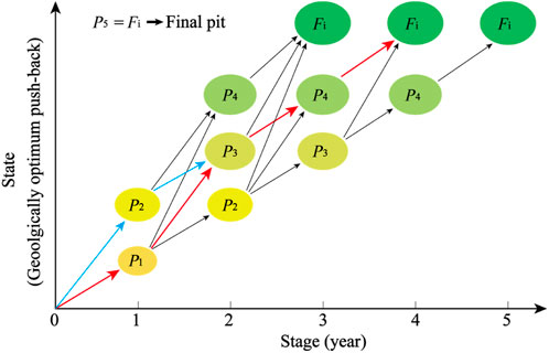
FIGURE 3. The dynamic programming scheme for push-back.

If the fuzzy NPV of path { p₀→p₁→p₃→F_i} in Figure 3 is the largest, the order of states on the path represents the optimal OPCMPS, and it can be seen that:

• The mining life is 3 years (the end of the third year push to the final mining final pit F_i.)

• State sequence. Push-back to state p₁ at the end of the first year; Push-back to state p₃ at the end of the second year; And push-back to state p₅ at the end of the third year.

• Through Eq. 13, it can be obtained that the fuzzy coal mining volume at the end of the 1st, 2nd, and 3rd year are ${\underset{\sim }{q}}_1$, ${\underset{\sim }{q}}_3-{\underset{\sim }{q}}_1$ and ${\underset{\sim }{q}}_5-{\underset{\sim }{q}}_3$ respectively. It can be obtained through Eq. 15 that the fuzzy stripping volume at the end of the 1st, 2nd, and 3rd year are ${\underset{\sim }{w}}_1$, ${\underset{\sim }{w}}_3-{\underset{\sim }{w}}_1$ and ${\underset{\sim }{w}}_5-{\underset{\sim }{w}}_3$ respectively. Similarly, the fuzzy profit and the fuzzy NPV of state transferred can be obtained by using Eqs. 17, 19 respectively. Finally, the flow chart of the dynamic optimization of OPCMPS with the proposed method is shown in Figure 4.

FIGURE 4

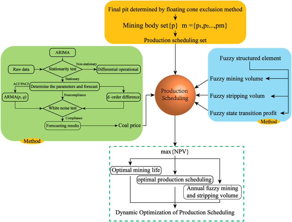
FIGURE 4. Dynamic optimization of OPCMPS flow.

6 Application of the proposed optimization approach to a large open-pit coal mine

6.1 Case background

The Chenbaerhuqi coal field in Hulunbuir City, Inner Mongolia Autonomous Region of China, is where the Baorixile open-pit mine is situated (as shown in Figure 5). The mine’s external perimeter spans a 50.72 km² region, measuring 5.86 km in width from north to south and 10.98 km in length from east to west. The mining adopts semi-continuous technology of single bucket excavator—dump truck—semi-fixed crushing station—belt conveyor, the stripping adopts discontinuous technology of single bucket excavator—dump truck—bulldozer. The whole open-pit mine is split into 5 mining regions based on careful consideration of the immediate economic advantages, long-term development of the open-pit mine, and the relationship between production continuity across mining areas. Figure 6 shows each mining area’s location and mining order. There are a total of five near-horizontal coal seams that can be mined. The coal volume still recoverable as of 31 December 2021, is 860.66 Mt. Baorixile open-pit coal mine has completed the mining task of the second mining area, and is making a production transition to the third mining area and the fourth mining area. However, during the turning period of the mining area, it is faced with the problem of difficult production connections. It is necessary to carry out a reasonable life cycle OPCMPS task based on the current situation.

FIGURE 5

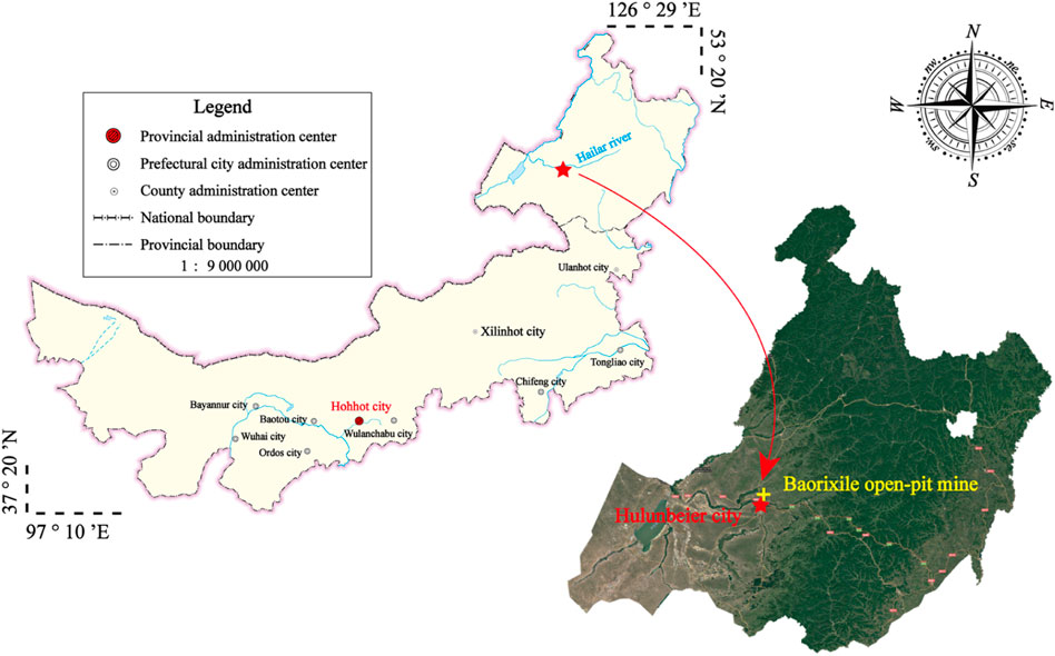
FIGURE 5. The location of the Baorixile open-pit mine.

FIGURE 6

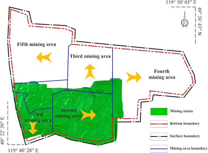
FIGURE 6. The mining area division of the Baorixile open-pit coal mine.

6.2 Time series prediction of coal price parameters

ARIMA model refers to the model established by transforming non-stationary time series into stationary time series and then regressing the lag value of a dependent variable with the current value and lag value of the error term. The actual historical coal sales prices of the mine from the first quarter of 2009 to the second quarter of 2022 were gathered as the basic data for the time series prediction analysis of coal sales prices through coordination and communication with the staff of the Zhanihe Open-pit Coal Mine’s production technology department. The coal price sequence is shown in Figure 7, and determines whether the sequence is stable.

FIGURE 7

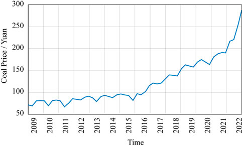
FIGURE 7. Coal price (2009Q1-2022Q2).

It can be seen from Figure 7 that the change in coal price fluctuates seasonally, and its trend is rising. The time series of prices does not have the characteristics of zero mean, and its variance is constantly changing, so it can be preliminarily determined that the time series of coal price is unstable.

In Figure 8; Table 1, it can be found that the decline rate of the autocorrelation coefficient is very slow. The autocorrelation coefficient before the 13 period is always outside the confidence interval. The partial autocorrelation coefficient decreases greatly after the first lag period and is not statistically significant. The autocorrelation coefficient value CA and the partial autocorrelation coefficient value CPA do not appear truncation and tailing, which further illustrates that the coal price time series is non-stationary.

FIGURE 8

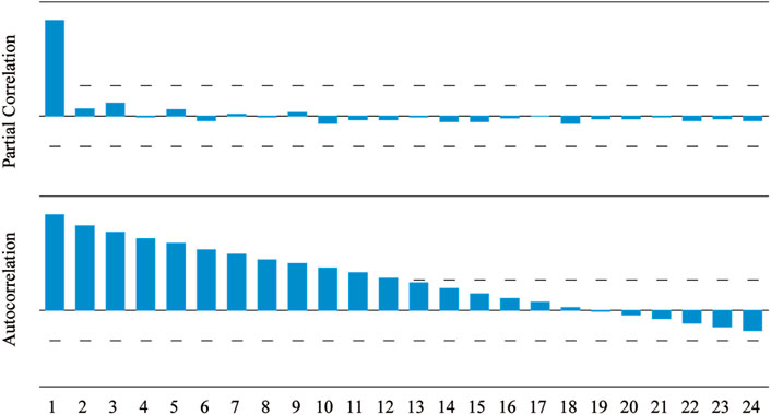
FIGURE 8. Stationarity test of the coal price time series.

TABLE 1

TABLE 1. Autocorrelation and Partial Correlation coefficient of the coal prices series.

The differential processing of coal price time series is to eliminate the fluctuation and the dependence on time, so that the data tends to be stable. The unit root test results after differential processing are shown in Tables 2, 3. After the first-order difference, the unit root test is performed, and the results show that there is a unit root, and p>0.05. The first-order difference sequence is unstable. After the second-order difference, the unit root test is performed, and the results showed no unit root and the p<0.05. After the second-order difference sequence is stable. Therefore, I = 2 in the ARIMA model.

TABLE 2

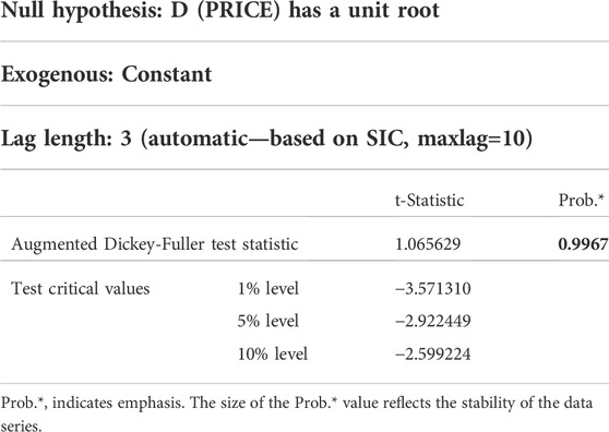
TABLE 2. The unit root test of first-order difference sequence.

TABLE 3

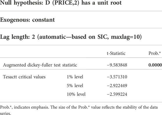
TABLE 3. The unit root test of second-order difference sequence.

Figure 9 shows that the second-order difference sequence is a stationary sequence with zero mean and variance. In Figure 10; Table 4, it can be seen that the image of the partial autocorrelation coefficient starts from p = 4, suddenly approaches the centre line, and hovers on both sides of the zero value. Therefore, it can be preliminarily concluded that the p is obtained on the (He et al., 2006; Wang et al., 2022). Similarly, through the change trend of the autocorrelation coefficient, it can be basically determined that the q is obtained on the (Ramazan, 2007; Wang et al., 2022), which can constitute ARIMA (1,2,1), ARIMA (1,2,2), ARIMA (1,2,3), ARIMA (1,2,4), ARIMA (2,2,1), ARIMA (2,2,2), ARIMA (2,2,3), ARIMA (2,2,4), ARIMA (3,2,1), ARIMA (3,2,2), ARIMA (3,2,3), ARIMA (3,2,4) these 12 models. Then by comparing the AIC, SC, MAPE and RMSE of each ARIMA model, an optimal coal price forecasting model is determined.

FIGURE 9

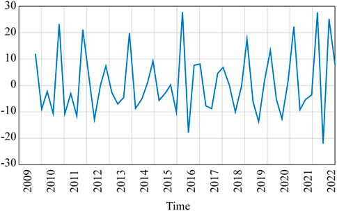
FIGURE 9. Second-order difference results of coal price time series.

FIGURE 10

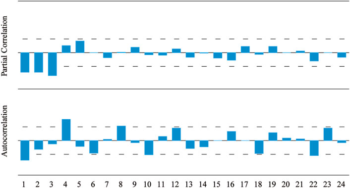
FIGURE 10. Stationarity test of the Second-order difference results.

TABLE 4

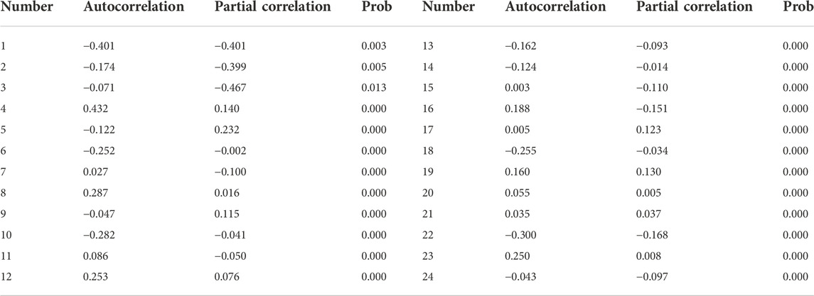
TABLE 4. Autocorrelation and Partial Correlation coefficient of the Second-order difference results.

Table 5 shows that the ARIMA (2, 2, 1) model has the largest corrected Adjusted-R² and the smallest AIC, SC, MAPE, and RMSE. Therefore, ARIMA (2, 2, 1) is tentatively used as the prediction model of coal price. However, coal price has some seasonal fluctuations, the difference needs to lag 4 to eliminate the impact of seasonal fluctuations. The calculated results are shown in Table 2.

TABLE 5

TABLE 5. The parameter comparison of each model’s test index.

Table 6 shows that the ARIMA (1, 2, 4) model has the highest corrected Adjusted-R² and the lowest AIC, SC, MAPE, and RMSE values across all models. Therefore, ARIMA (1, 2, 4) is used as the prediction model of coal price.

TABLE 6

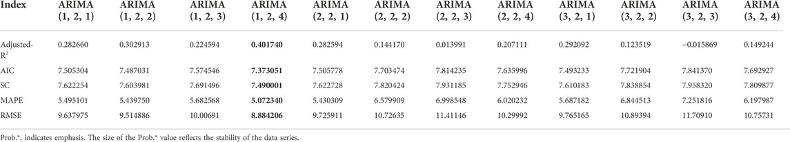
TABLE 6. The parameter comparison of each model’s test index (eliminate seasonal fluctuations).

Figure 11 shows that the effect of using this model to predict the coal price is better, but the effect of short-term prediction will be better. The ARIMA model only considers the characteristics of the coal price time series itself, without considering the influence of some uncertain factors. With the extension of the test time, the prediction error of the model will also increase. Therefore, with the growth of the year, the sample data of coal price prediction can be dynamically updated every year to achieve more accurate prediction results of future coal prices. This model is used to predict the coal price in the next 23 years. The result of coal price forecast based on ARIMA (1, 2, 4) is shown in the red curve Figure 12.

FIGURE 11

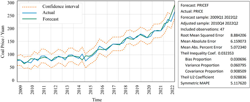
FIGURE 11. The result of the coal prediction model based on ARIMA.

FIGURE 12

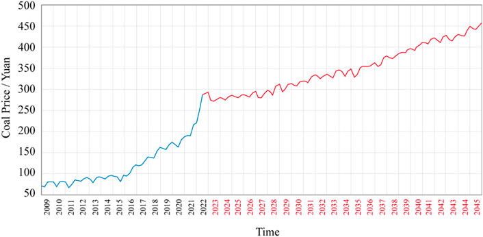
FIGURE 12. The result of coal price forecast in the next 23 years based on ARIMA.

6.3 Application of proposed optimization approach

In the preparation of the OPCMPS process, according to the actual situation of the mine, set the mining body of coal increment of about 2.3 million tons, the recovery rate of 95%, stop working slope angle of 8°, and the annual production capacity of about 25 million tons. The production cost of coal mining is 96.27 yuan/t, the stripping cost is 7 yuan/m³, the price of raw coal is 220.25 yuan/t, the cost rise rate is 3%, the price rise rate is 5%, and the annual discount rate is 7.5%. The coal price predicted by ARIMA is combined with the dynamic sorting of the geological optimal mining body based on the structural element theory proposed in this paper.

AutoCAD is a popular computer-aided design (CAD) and drawing software program. By autodesk, who also developed and sold it. The AutoCAD application is a great and well-liked tool that creates any sort of schemes and drawings with high precision and quality. Additionally, it aids in fully recognizing the creative potential of program users. In order to automate their design work, millions of professionals, scientists, engineers, and students now often utilize the AutoCAD system (Cao and Miyamoto, 2003). Based on AutoCAD, the secondary development is carried out to establish a three-dimensional deposit block model, and a total of 128 geological optimal mining bodies are generated.

Taking E as a triangular structure element, Its membership function is $E\left(x\right)=\{\begin{array}{l}1+x,-1\le x\le 0\\ 1-x,0\le x\le 1\end{array}$, The fuzzy mining quantity and fuzzy stripping quantity of 128 geological optimal mining bodies can be expressed by the triangular fuzzy number. Taking No. 1 geologically optimal mining body as an example, let $f\left(x\right)=2419.83+0.18x$, $g_1\left(x\right)=2419.83+0.18x$, then $q_1\left(x\right)=f_1\left(E\right)=2419.83+0.18E$, $w_1=g_1\left(E\right)=11784.57+0.85E$. Others can be analogized. Let $p_t=0.022{\left(1+0.05\right)}^t$, $c_t=0.0096{\left(1+0.03\right)}^t$, $b_t=0.0007{\left(1+0.03\right)}^t$, $d=0.0075$, $z_t=0.001+0.001h_t$, $h_t$ is calculated according to the specific situation of the mining body. Therefore, according to the fuzzy coal mining amount, fuzzy stripping amount and set technical parameters, the software is used to perform fuzzy dynamic sorting on the sequence composed of 128 geological optimal mining bodies. The optimization results of OPCMPS are shown in Table 3.

Table 7 shows that when the sequence of geologically optimal mining body is {p₁ → p₁₅ → p₂₄→ _…→ p₉₈ → p₁₁₀ → p₁₂₈}, the maximum fuzzy total NPV is (418453.714+31.1163E) ×10⁴ yuan. It can be seen that the optimal mining life is 23 years. The annual amount of fuzzy coal mining and stripping can be determined in Table 3. The membership degree of fuzzy total NPV is:

$u_{N\underset{\sim }{P}{V}_{\left(\mathrm{32,128}\right)}}\left(x\right)=\{\begin{array}{l}1+\frac{x-418453.714}{31.1163};418422.5977\le x\le 418453.714\\ 1-\frac{x-418453.714}{31.1163};418453.714\le x\le 418484.8303\end{array}$

TABLE 7

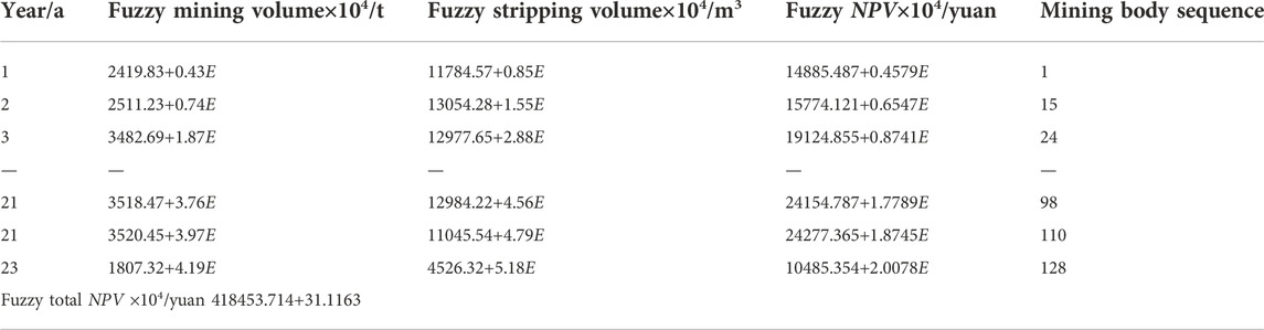
TABLE 7. The optimization results of OPCMPS.

In addition to the first and 2nd years when the mining field is in the turning period of the mining area and the last year when the mining task is completed, the annual fuzzy coal mining volume fluctuates greatly. Others are 35 million tons.

7 Discussions

There have been many studies on production scheduling in the field of open-pit metal mines, but there have been very few studies in this area for open-pit coal mines with stratified ore bodies. From the viewpoint of fuzzy economics, this study suggests a novel mathematical model of the total NPV of opencast coal mine production scheduling, while the majority of other studies on this topic have been built by taking into account various limitations. Additionally, this study offers a method for projecting coal prices based on economic time series, and it dynamically executes the production scheduling optimization design from a dynamic economics perspective to account for the effects of price fluctuations on the total NPV. The novel approach that has been suggested would undoubtedly aid in the design and construction of open-pit coal mines and offer fresh perspectives to experts working in this area. Additionally, the production schedule optimization technique suggested in this study can be used as a guide for open-pit metal miners.

The size of the sample data set will have an impact on the forecast accuracy, which is one drawback of the price prediction approach. This paper’s case study research findings demonstrate that the proposed production scheduling model may simultaneously achieve the best production capacity, excavation order, and production life. But because the mine only began selling coal in 2009, there is only a limited sample data set that can be used to anticipate coal prices. However, there is a technique for optimization and adjustment, which allows for the correction of the current year’s coal price and the dynamic updating and adjusting of the future production schedule throughout the development and building of mines.

8 Conclusion

The traditional optimization method of OPCMPS adopts accurate calculation, which somewhat ignores the mining process’s uncertainty. Based on the production scheduling optimization method proposed in Reference (Gu et al., 2011), this paper introduces the fuzzy structural element theory to establish the fuzzy optimization model of fuzzy coal mining volume, fuzzy stripping volume and fuzzy total NPV and their respective membership function expressions. At the same time, considering the volatility of coal prices over time, the ARIMA prediction model is used for prediction. Through the analysis of coal prices from 2009 to 2022, the prediction model was determined as ARIMA (1, 2, 4), and the model was applied to predict coal prices in the next 23 years. The optimal mining sequence of the optimal geological body and the fuzzy coal mining volume, fuzzy stripping volume and fuzzy NPV of each optimal geological body is obtained by combining the constructed fuzzy optimization model, the predicted coal price and the moving cone exclusion method. The maximum total NPV is (418453.714 + 31.1163 E) × 10⁴ yuan, and the optimal mining period of the mine is 23 years.

Data availability statement

The original contributions presented in the study are included in the article/supplementary material, further inquiries can be directed to the corresponding author.

Author contributions

All authors listed have made a substantial, direct, and intellectual contribution to the work and approved it for publication.

Funding

This research was supported by the National Natural Science Foundation of China (Grant no. 51974144) and the Discipline Innovation Team of Liaoning Technical University (LNTU20TD-07). The “Jie Bang Gua Shuai” (Take the Lead) of the Key Scientific and Technological Project for Liaoning Province additionally provided financial assistance for this study under the grant number [2021JH1/10400011].

Conflict of interest

The author CY was employed by National Energy Investment Group Co. Ltd.

The remaining authors declare that the research was conducted in the absence of any commercial or financial relationships that could be construed as a potential conflict of interest.

Publisher’s note

All claims expressed in this article are solely those of the authors and do not necessarily represent those of their affiliated organizations, or those of the publisher, the editors and the reviewers. Any product that may be evaluated in this article, or claim that may be made by its manufacturer, is not guaranteed or endorsed by the publisher.

References

Alipour, A., Khodaiari, A. A., Jafari, A., and Tavakkoli-Moghaddam, R. (2020). Production scheduling of open-pit mines using genetic algorithm: A case study. Int. J. Manag. Sci. Eng. Manag. 15 (3), 176–183. doi:10.1080/17509653.2019.1683090

CrossRef Full Text | Google Scholar

Bienstock, D., and Zuckerberg, M. (2009). A new LP algorithm for precedence constrained production scheduling. Optim. Online, 1–33.

Google Scholar

Blom, M., Pearce, A. R., and Stuckey, P. J. (2018). Multi-objective short-term production scheduling for open-pit mines: A hierarchical decomposition-based algorithm. Eng. Optim. 50 (12), 2143–2160. doi:10.1080/0305215x.2018.1429601

CrossRef Full Text | Google Scholar

Blom, M., Pearce, A. R., and Stuckey, P. J. (2017). Short-term scheduling of an open-pit mine with multiple objectives. Eng. Optim. 49 (5), 777–795. doi:10.1080/0305215x.2016.1218002

CrossRef Full Text | Google Scholar

Boland, N., Dumitrescu, I., Froyland, G., and Gleixner, A. M. (2009). LP-based disaggregation approaches to solving the open pit mining production scheduling problem with block processing selectivity. Comput. Operations Res. 36 (4), 1064–1089. doi:10.1016/j.cor.2007.12.006

CrossRef Full Text | Google Scholar

Box, G. E. P., Jenkins, G. M., and Reinsel, G. C., (2015). Time series analysis: Forecasting and control. Hoboken, New Jersey, United States: John Wiley & Sons.

Google Scholar

Caccetta, L., and Hill, S. P. (2003). An application of branch and cut to open pit mine scheduling. J. Glob. Optim. 27 (2), 349–365. doi:10.1023/a:1024835022186

CrossRef Full Text | Google Scholar

Cao, W., and Miyamoto, Y. (2003). Direct slicing from AutoCAD solid models for rapid prototyping. Int. J. Adv. Manuf. Technol. 21 (10), 739–742. doi:10.1007/s00170-002-1316-0

CrossRef Full Text | Google Scholar

Chicoisne, R., Espinoza, D., Goycoolea, M., Moreno, E., and Rubio, E. (2012). A new algorithm for the open-pit mine production scheduling problem. Operations Res. 60 (3), 517–528. doi:10.1287/opre.1120.1050

CrossRef Full Text | Google Scholar

Clements, M. P., and Hendry, D. F. (1998). Forecasting economic time series. Cambridge, United Kingdom: Cambridge University Press.

Google Scholar

Contreras, J., Espinola, R., Nogales, F. J., and Conejo, A. (2003). ARIMA models to predict next-day electricity prices. IEEE Trans. Power Syst. 18 (3), 1014–1020. doi:10.1109/tpwrs.2002.804943

CrossRef Full Text | Google Scholar

Eivazy, H., and Askari-Nasab, H. (2012). A mixed integer linear programming model for short-term open pit mine production scheduling. Min. Technol. 121 (2), 97–108. doi:10.1179/1743286312y.0000000006

CrossRef Full Text | Google Scholar

Fathollahzadeh, K., Mardaneh, E., Cigla, M., and Asad, M. W. A. (2021). A mathematical model for open pit mine production scheduling with Grade Engineering® and stockpiling. Int. J. Min. Sci. Technol. 31 (4), 717–728. doi:10.1016/j.ijmst.2021.03.011

CrossRef Full Text | Google Scholar

Fytas, K. (1986). “A computerized model of open pit short and long range production scheduling,” in Proceeding of the 19th A PCOM Symposium (SME-AME), New York, 109–119.

Google Scholar

Gilani, S. O., Sattarvand, J., Hajihassani, M., and Abdullah, S. S. (2020). A stochastic particle swarm based model for long term production planning of open pit mines considering the geological uncertainty. Resour. Policy 68, 101738. doi:10.1016/j.resourpol.2020.101738

CrossRef Full Text | Google Scholar

Gu, X. W., Wang, P. F., Wang, Q., Zheng, Y. Y., Liu, J. P., and Chen, B. (2011). Simultaneous optimization of final pit and production schedule in open-pit coal mines. Adv. Mat. Res. 323, 222–228. doi:10.4028/www.scientific.net/AMR.323.222

CrossRef Full Text | Google Scholar

Guo, S. C. (2009). Comparison and ordering of fuzzy numbers based on method of structured element. Syst. Eng. - Theory & Pract. 29 (3), 106–111. doi:10.1016/s1874-8651(10)60013-0

CrossRef Full Text | Google Scholar

Guo, S. C. (2002a). Method of structuring element in fuzzy analysis (I). Fuxin: Journal of Liaoning Technical University, 670–673.

Google Scholar

Guo, S. C. (2002b). Method of structuring element in fuzzy analysis (II). Fuxin: Journal of Liaoning Technical University, 808–810.

Google Scholar

Guo, S. C., and Song, T. (2011). Operations and measurement of interval-valued fuzzy numbers based on the method of structured element. Fuzzy Inf. Eng. 3 (1), 101–110. doi:10.1007/s12543-011-0069-6

CrossRef Full Text | Google Scholar

Harvey, A. C. (1990). Forecasting, structural time series models and the Kalman filter, Cambridge, UK: Cambridge University Press.

Google Scholar

He, G. J., Liu, S. S., Si, l., Gao, Q., Ma, J., and Zhao, J. L. (2006). Study on coal cost of major coal-producing countries abroad. Selected articles on coal economics in 2006, 177–270. Beijing: China Coal Industry Publishing House.

Google Scholar

Hendry, D. F., and Doornik, J. A. (1994). Modelling linear dynamic econometric systems[J]. Scott. J. Polit. Econ. 41 (1), 1–33. doi:10.1111/j.1467-9485.1994.tb01107.x

CrossRef Full Text | Google Scholar

Jiang, S., Yang, C., Guo, J., and Ding, Z. (2018). ARIMA forecasting of China’s coal consumption, price and investment by 2030. Energy Sources, Part B Econ. Plan. Policy 13 (3), 190–195. doi:10.1080/15567249.2017.1423413

CrossRef Full Text | Google Scholar

Khan, A., and Niemann-Delius, C. (2018). A Differential Evolution based approach for the production scheduling of open pit mines with or without the condition of grade uncertainty. Appl. Soft Comput. 66, 428–437. doi:10.1016/j.asoc.2018.02.010

CrossRef Full Text | Google Scholar

Khan, A. (2018). Long-term production scheduling of open pit mines using particle swarm and bat algorithms under grade uncertainty. J. South. Afr. Inst. Min. Metall. 118 (4), 361–368. doi:10.17159/2411-9717/2018/v118n4a5

CrossRef Full Text | Google Scholar

Li, H. (2021). Prediction of coal price based on ARIMA model. Front. Econ. Manag. 2 (8), 155–163. doi:10.9734/ajeba/2022/v22i830590

CrossRef Full Text | Google Scholar

Li, K., and Lin, B. (2017). Economic growth model, structural transformation, and green productivity in China. Appl. Energy 187, 489–500. doi:10.1016/j.apenergy.2016.11.075

CrossRef Full Text | Google Scholar

Liu, X. (2021). Research on the forecast of coal price based on LSTM with improved Adam optimizer. J. Phys. Conf. Ser. 1941 (1), 012069. doi:10.1088/1742-6596/1941/1/012069

CrossRef Full Text | Google Scholar

Nelson, L. R., and Goldstern, M. R. (1980). “Interactive short range mine planning a case study,” in Weiss a Computer Methods for the 80’s in the Mineral Industry (SME-AME), New York: AIME, 592–600.

Google Scholar

Osanloo, M., Gholamnejad, J., and Karimi, B. (2008). Long-term open pit mine production planning: A review of models and algorithms. Int. J. Min. Reclam. Environ. 22 (1), 3–35. doi:10.1080/17480930601118947

CrossRef Full Text | Google Scholar

Ramazan, S. (2007). The new fundamental tree algorithm for production scheduling of open pit mines. Eur. J. Operational Res. 177 (2), 1153–1166. doi:10.1016/j.ejor.2005.12.035

CrossRef Full Text | Google Scholar

Tolouei, K., Moosavi, E., Bangian Tabrizi, A. H., and Afzal, P. (2021). Application of an improved Lagrangian relaxation approach in the constrained long-term production scheduling problem under grade uncertainty. Eng. Optim. 53 (5), 735–753. doi:10.1080/0305215x.2020.1746295

CrossRef Full Text | Google Scholar

Tolouei, K., Moosavi, E., Tabrizi, A. H. B., Afzal, P., and Bazzazi, A. A. (2021). An optimisation approach for uncertainty-based long-term production scheduling in open-pit mines using meta-heuristic algorithms. Int. J. Min. Reclam. Environ. 35 (2), 115–140. doi:10.1080/17480930.2020.1773119

CrossRef Full Text | Google Scholar

Turan, G., and Onur, A. H. (2022). Optimization of open-pit mine design and production planning with an improved floating cone algorithm. Optim. Eng., 1–25. doi:10.1007/s11081-022-09725-4

CrossRef Full Text | Google Scholar

Upadhyay, S. P., and Askari-Nasab, H. (2018). Simulation and optimization approach for uncertainty-based short-term planning in open pit mines. Int. J. Min. Sci. Technol. 28 (2), 153–166. doi:10.1016/j.ijmst.2017.12.003

CrossRef Full Text | Google Scholar

Wang, L. L., Li, Y., Zhang, J. J., Qian, M., and Cao, Y. (2022). Analysis on the difference of reconstructed soil moisture content in a grassland open-pit mining area of China. Agronomy 12 (5), 1061. doi:10.3390/agronomy12051061

CrossRef Full Text | Google Scholar

Wang, X., Liu, C., Chen, S., Chen, L., and Li, K. (2020). Impact of coal sector’s de-capacity policy on coal price. Appl. Energy 265, 114802. doi:10.1016/j.apenergy.2020.114802

CrossRef Full Text | Google Scholar

Zhang, X., Liu, C., and Qian, Y. (2020). Coal price forecast based on ARIMA model. Fin. For. 9 (4), 180. doi:10.18282/ff.v9i4.1530

CrossRef Full Text | Google Scholar

Zheng, F. W., Zhen, X., and Chen, C. X. (2014). Development status and trend of world open-pit coal mine. Chain Coal 40, 113–116. doi:10.19880/j.cnki.ccm.2014.11.028

CrossRef Full Text | Google Scholar