Estimation of the ground-level SO2 concentration in eastern China based on the LightGBM model and Himawari-8 TOAR

Sulfur dioxide (SO₂) is one of the main pollutants in China’s atmosphere, but the spatial distribution of ground-based SO₂ monitors is too sparse to provide a complete coverage. Therefore, obtaining a high spatial resolution of SO₂ concentration is of great significance for SO₂ pollution control. In this study, based on the LightGBM machine learning model, combined with the top-of-atmosphere radiation (TOAR) of Himawari-8 and additional data such as meteorological factors and geographic information, a high temporal and spatial resolution TOAR-SO₂ estimation model in eastern China (97–136°E, 15–54°N) is established. TOAR and meteorological factors are the two variables that contribute the most to the model, and both of their feature importance values exceed 30%. The TOAR-SO₂ model has great performance in estimating ground-level SO₂ concentrations with 10-fold cross validation R² (RMSE) of 0.70 (16.26 μg/m³), 0.75 (12.51 μg/m³), 0.96 (2.75 μg/m³), 0.97 (2.16 μg/m³), and 0.97 (1.71 μg/m³) when estimating hourly, daily, monthly, seasonal, and annual average SO₂. Taking North China as main study area, the annual average SO₂ is estimated. The concentration of SO₂ in North China showed a downward trend since 2016 and decreased to 15.19 μg/m³ in 2020. The good agreement between ground measured and model estimated SO₂ concentrations highlights the capability and advantage of using the model to monitor spatiotemporal variations of SO₂ in Eastern China.

1 Introduction

In past decades, China’s industrialization has accelerated, resulting in more serious environmental problems (Li et al., 2014). SO₂ is a primary source of air pollution and directly affects human health, causing various cardiovascular and respiratory diseases (Sunyer, 2003; Johns and Linn, 2011; Li et al., 2015; Song et al., 2016; Wang et al., 2018). In addition, as a main precursor of sulfate, SO₂ increases the frequency of haze events and causes substantial damage to the ecological environment (Zhu et al., 2011; Lee, 2015; Calkins et al., 2016).

In recent years, China has successively built a series of SO₂ ground monitoring stations. These stations can provide data sources for SO₂-related research. However, the small number and uneven distribution render limited spatial coverage of ground-based SO₂ monitors (Yu et al., 2018). Compared with ground monitoring, satellite observation has a wide coverage, and there is a good correlation between SO₂ column concentration and ground-level SO₂ concentration, mainly using polar orbiting satellites. Therefore, the model based on SO₂ column concentration from satellite observation has become an effective tool to obtain ground-level SO₂ concentration with high spatial resolution (Ialongo et al., 2016; Liu et al., 2016). At present, satellite instruments widely used in SO₂ column concentration monitoring are the Global Ozone Monitoring Experiment (GOME) (Eisinger and Burrows, 1998), the Atmospheric Infrared Sounder (AIRS) (Carn, 2005), the Ozone Monitoring Instrument (OMI) (Yang et al., 2007; Li et al., 2017; Zhang et al., 2017; Li et al., 2020a) and the Scanning Imaging Absorption Spectrometer for Atmospheric Chartography (SCIAMACHY) (Lee et al., 2011). Based on satellite remote sensing, these studies successfully estimated the ground-level SO₂ concentration using statistical methods, which filled the gap in observational data.

However, polar orbiting satellites can only observe daily data on the concentration of SO₂ columns, and these data are a combination of observations taken at two different times. That is to say, the input data to the model have low temporal resolution and are not observed at the same time. By comparison, some geostationary orbit satellites can observe panoramic TOAR once an hour. Himawari-8 is an advanced geostationary orbit satellite (Yoshida et al., 2018) launched by the Japan Meteorological Agency (JMA). Its TOAR data covers a wide area of eastern China with high temporal resolution, including 16 bands ranging from visible to near-infrared light. Therefore, the Himawari-8 TOAR has great advantages in building a high spatial and temporal resolution estimation model of ground-level pollutant concentration, which has been widely used in many related studies (Zang et al., 2018; Wei et al., 2021; Xu et al., 2021; Song et al., 2022a; Chen et al., 2022c). However, to the best of our knowledge, the Himawari-8 TOAR has not been applied to ground-level SO₂ concentration estimation so far.

Compared with statistical models, machine learning algorithms have better data processing ability for high-dimensional data and can better solve nonlinear relationships, providing it with better application prospects in SO₂ estimation (Tripathy et al., 2021). Therefore, this study aims to estimate ground-level SO₂ concentration in eastern China based on the Light Gradient Boosting Machine (LightGBM) machine learning model, combined with Himawari-8 TOAR and auxiliary data such as meteorological factors and geographic information.

2 Data and methods

2.1 Data

2.1.1 Ground SO₂ observations

The SO₂ ground observation data used in the study came from the National Environmental Quality Monitoring Center of China, which can be obtained from its official website at http://www.cnemc.cn/en/. The quality assurance and validity judgment of SO₂ data are controlled according to HJ818-2018 technical specification. The study area in this paper is the eastern China (97–136°E, 15–54°N), and hourly SO₂ data from approximately 1800 SO₂ ground monitoring stations from 1 September 2015, to 31 August 2021, are used. The spatial distribution of these stations is shown in Figure 1. It can be seen that the stations are only sparsely distributed in the west and north of the study area.

FIGURE 1

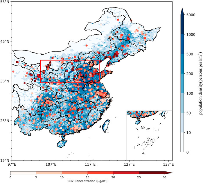
FIGURE 1. Distribution map of SO₂ monitoring stations. The color of the stations indicates the hourly average SO₂ concentration of the ground observation site. The bottom map shows the population density distribution. The area in the red box in the figure is North China, which is the most polluted region in eastern China.

2.1.2 Himawari-8 TOAR

Himawari-8, the world’s first geostationary weather satellite capable of obtaining color images, was launched by JMA in 2014, and data became available in 2015. The Advanced Himawari Imager (AHI) contains a total of 16 bands from visible light to near-infrared wavelengths, named B1, B2, B3, B4, B5, B6, B7, B8, B9, B10, B11, B12, B13, B14, B15, and B16, respectively (Yoshida et al., 2018). Details of 16 bands information of the Advanced Himawari Imager (AHI) instrument on Himawari-8 satellite is shown in Table 1. However, the observation range of Himawari-8 is limited to 80°E −200°E and 60°S-60°N, so no valid data can be obtained in China’s Tibet, Xinjiang and western Sichuan (Song et al., 2022a). The Himawari-8 TOAR data used in this paper have a temporal resolution of 1 h and a spatial resolution of 5 km.

TABLE 1

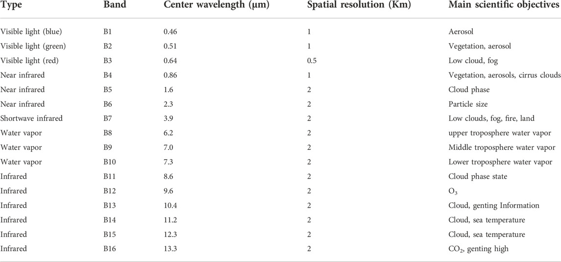
TABLE 1. Details of 16 bands information of the Advanced Himawari Imager (AHI) instrument on Himawari-8 satellite.

2.1.3 Meteorological factors and geographic information

Considering that meteorological conditions will affect the formation, accumulation and diffusion of SO₂ (He et al., 2017), various meteorological factor values are added to the model. The meteorological factors used in this study are from the European Centre for Medium-Range Weather Forecasts (ECMWF) EAR-5 reanalysis datasets (Hersbach et al., 2020), which have an hourly temporal resolution and a spatial resolution of 0.25°×0.25° or 0.1°×0.1° (as Table 2 showed). Meteorological factors used in this study mainly include boundary layer height (BLH), relative humidity (RH), surface pressure (SP), 2 m temperature (TM), and 10 m U and V winds (U₁₀, V₁₀) (Li et al., 2019b; Song et al., 2022b). In addition to meteorological factors, geographic information also affects SO₂ concentrations. The geographic information selected in this paper mainly includes land cover type (LUCC), altitude (height) and population density (pd). LUCC is represented by high and low vegetation indices (LH, LL) from EAR-5, height is from SRTM-3 data (spatial resolution of 90 m) jointly measured by NASA and the National Imaging and Mapping Agency (NIMA), and pd is from NASA Socioeconomic Data and Application Center (spatial resolution of 0.04°×0.04°). The distribution of population density in eastern China is shown in Figure 1.

TABLE 2

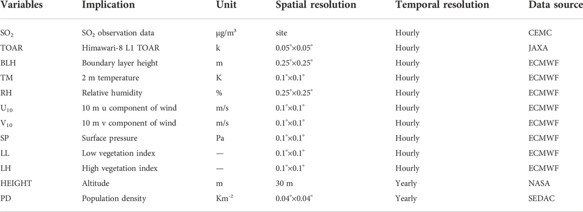
TABLE 2. Details of the data used in the study.

2.2 Methods

2.2.1 Data matching

First, through the bilinear interpolation method, the spatial resolution of various meteorological factors and geographic information is adjusted to be consistent with the grid resolution of Himawari-8 (0.05°×0.05°). Then, hourly SO₂ ground station observations are matched against the established grid. If there is one station in the grid, the observed value of the station is the data for that grid, and if there is more than one station in the grid, the average of the data from these stations is the grid value. The latitude and longitude range of the study area after data matching is 97–136°E, 15–54°N; the study area, contains a total of 6,087,672 data points.

2.2.2 Bands selection

After testing, we find that when the feature importance of a variable is less than 2%, it will not only degrade the model performance, but also increase the computation amount, which wastes the storage space and running time. Therefore, we take 2% as the threshold of feature importance to select TOAR bands. It should be noted that the feature importance only represents the contribution of each variable to the model, but cannot represent the physical reasons why these variables affect the ground-level SO₂ concentrations. In this way, we pick out suitable bands in each season as part of the input data. Figure 2 shows the feature importance for Himawari-8 satellite bands in the models of four seasons. Based on the results of Figure 2, the final bands are selected as Table 3.

FIGURE 2

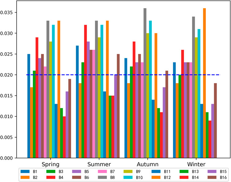
FIGURE 2. Feature importance for Himawari-8 satellite bands in the models of four seasons, where the blue dashed line represents the x=0.02 line.

TABLE 3

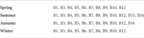
TABLE 3. Bands selected by the model in different seasons.

2.2.3 Light gradient boosting machine

LightGBM is a decision tree algorithm based on the histogram algorithm. Its main idea is still to use weak classifier (decision tree) iterative training to obtain the optimal model, but two new technologies gradient-based one-side sampling (GOSS) and exclusive feature bundling (EFB) are added, which allows it to quickly record data characteristics (Ke et al., 2017). At the same time, LightGBM uses a depth-limited leafwise algorithm to filter out leaf splits with low gain, reducing the algorithm overhead. It is precisely based on these optimizations that LightGBM can save considerable running time and storage space compared with the traditional decision tree algorithm to achieve the purpose of rapidly processing massive data (Ma et al., 2022).

The model performance is described by three indicators: coefficient of determination (R²), mean absolute error (MAE), and root mean square error (RMSE). Their definitions are as follows (Chen et al., 2022b):

${\mathit{R}}^{\mathbf{2}}=\mathbf{1}-\frac{{{\sum }_{\mathit{i}=\mathbf{1}}^{\mathit{n}}({\widehat{\mathit{y}}}_{\mathit{i}}-{\mathit{y}}_{\mathit{i}})}^{\mathbf{2}}}{{{\sum }_{\mathit{i}=\mathbf{1}}^{\mathit{n}}({\mathit{y}}_{\mathit{i}}-\overline{\mathit{y}})}^{\mathbf{2}}}(1)$

$\mathit{M}\mathit{A}\mathit{E}=\frac{\mathbf{1}}{\mathit{n}}{\sum }_{\mathit{i}=\mathbf{1}}^{\mathit{n}}|{\widehat{\mathit{y}}}_{\mathit{i}}-{\mathit{y}}_{\mathit{i}}|(2)$

$\mathit{R}\mathit{M}\mathit{S}\mathit{E}=\sqrt{\frac{\mathbf{1}}{\mathit{n}}{{\sum }_{\mathit{i}=\mathbf{1}}^{\mathit{n}}({\widehat{\mathit{y}}}_{\mathit{i}}-{\mathit{y}}_{\mathit{i}})}^{\mathbf{2}}}(3)$

where ${\widehat{\mathit{y}}}_{\mathit{i}}$ represents the predicted value of the model, ${\mathit{y}}_{\mathit{i}}$ represents the true value, $\overline{y}$ represents the mean of the true value, and n represents the total sample.

In this study, the comparison between the performance of LightGBM and other machine learning models in Himawari-8 TOAR data is shown in Table 4. We choose LightGBM model in this study because of its good performance and short running time.

TABLE 4

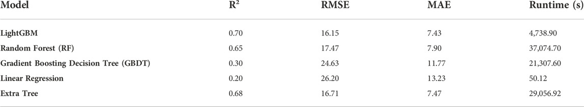
TABLE 4. Performances Comparisons of Machine Models in Himawari-8 TOAR data.

3 Results and discussion

3.1 Model cross validation results

To test the performance of the model, we apply 10-fold cross validation (Chen et al., 2019; Chen et al., 2022a). The data is split into ten parts, nine for training the model and one for validating the results, and the process is repeated ten times. Based on 9:00–16:00 (this article uses Beijing time, which is 8 h earlier than Universal Time), the 10-fold cross validation result of the validation dataset is shown in Figure 3. R² is 0.64–0.72, RMSE is 11.89 μg/m³-19.9 μg/m³, MAE is 5.56 μg/m³-9.65 μg/m³, and the fitting slope is 0.62–0.69. The results estimated by the model are slightly lower than the observations. During the time period of 9:00–16:00, the performance of the model varies with time. Generally, it shows a trend of first rising and then decreasing. The model performs best in the period of 13:00–14:00 (R² is 0.72). This is because meteorological conditions such as high temperature and atmospheric instability at noon are conducive to the diffusion of pollutants. And the solar radiation is strongest at this time, so the TOAR will also be stronger, thus generating the best radiation signal received by the satellite.

FIGURE 3

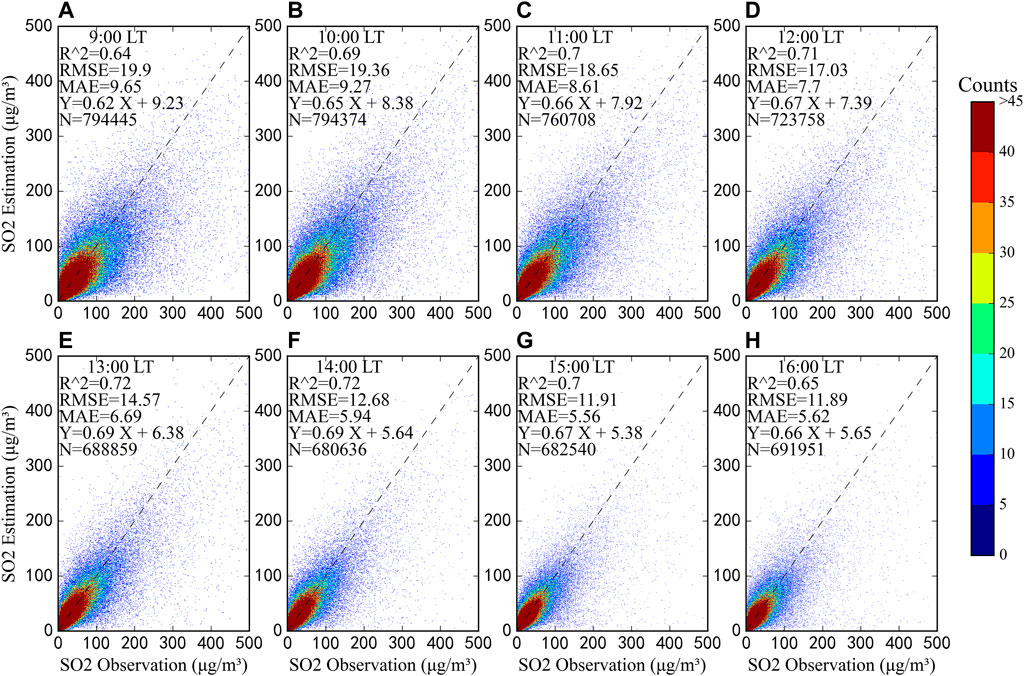
FIGURE 3. Hourly model 10-fold cross validation results based on samples, which the light dashed line is the perfectly fitted line, that is, the 1:1 relationship, LT represents Beijing time, and N represents the total sample amount.

As shown in Figures 4A–D, the model performs best in winter with a 10-fold cross validation R² of 0.72. Performance is the worse in summer with a R² value of only 0.51. R² in spring and autumn are 0.62 and 0.65. This may be related to the complex and changeable meteorological conditions in summer and the highest concentration of SO₂ in winter (Wei et al., 2019; Zang et al., 2019). Therefore, the TOAR-SO₂ model can effectively capture high SO₂ events in winter over eastern China.

FIGURE 4

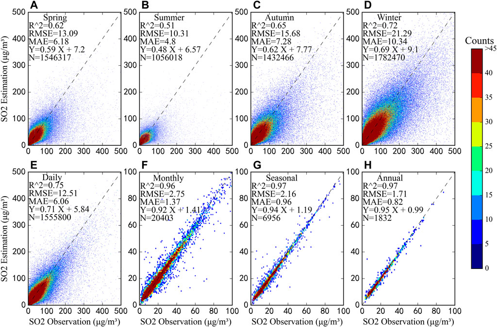
FIGURE 4. Similar to Figure 3, except for spring (A) summer (B) autumn (C) winter (D) daily (E) monthly (F) seasonal (G) and annual (H) average 10-fold cross validation results of Himawari-8 TOAR-SO₂ model based on samples.

The 10-fold cross validation results based on daily, monthly, seasonal, and annual average SO₂ are shown in Figures 4E–H. The performance of TOAR-SO₂ model has been significantly improved when estimating monthly, seasonal, and annual average SO₂ with R² (RMSE) of 0.96 (2.75 μg/m³), 0.97 (2.16 μg/m³) and 0.97 (1.71 μg/m³). In contrast, the model is ordinary when estimating the daily average SO₂, but R² (RMSE) can still reach 0.75 (12.51 μg/m³). It can be seen that the larger the time scale, the better the estimation effect of the TOAR-SO₂ model. This proves that using TOAR-SO₂ models to estimate SO₂ concentrations is reliable.

To test whether the model has better performance in regions with high annual average SO₂ concentrations, this paper conducts a 10-fold cross validation of 348 cities in eastern China with SO₂ ground-truth data records and then screened out the proportion of cities with R² values between 0.8 and 0.9, 0.7–0.8, 0.6–0.7, 0.5–0.6, and 0–0.5 in the top 20, top 50, top 100, top 150 cities and all cities in eastern China by pollution level from 2016 to 2020. In Figure 5, the results show that with the increase of SO₂ pollution, the proportion of cities with R² values between 0.8 and 0.9 increases significantly. At the same time, cities with R² values between 0.7 and 0.8 generally show the same but only 10% of these cities are among the top 20 polluted cities. The proportion of cities with R² values between 0.5 and 0.7 doesn’t change significantly. However, for cities with R² values lower than 0.5, the proportion of SO₂ decreases significantly with increasing SO₂ concentration. It can be seen that the model has a better estimation effect in areas with severe SO₂ pollution and the estimation result is basically close to the site data.

FIGURE 5

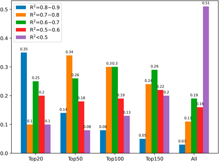
FIGURE 5. The proportion of cities with R² values in the top 20, top 50, top 100, and top 150 of SO₂ pollution cities and all cities in eastern China from 2016 to 2020.

In conclusion, the TOAR-SO₂ model established in this study can accurately estimate the SO₂ concentration in eastern China. The estimated result is slightly lower than the observation. The TOAR-SO₂ model performs best in winter and in areas with severe SO₂ pollution, and it works well when estimating monthly, seasonal, and annual average SO₂. Therefore, the SO₂ estimated by the TOAR-SO₂ model can provide reliable data for monitoring the spatial variation and temporal trend of SO₂ pollution in eastern China.

3.2 Feature importance of the TOAR-SO₂ model

The feature selection of the TOAR-SO₂ model adopts the backward selection method (Li et al., 2020b), that is, the variables with low feature importance are filtered out, and only the variables with high feature importance are retained. The feature importance of selected variables in each season is shown in Figure 6A. The results show that TOAR and meteorological factors are the two variables that contribute the most to the model, and both of their feature importance values exceed 30% in each season. The high feature importance of meteorological factors indicates that they have a great influence on SO₂ concentration (Xie et al., 2015; Liu et al., 2017). The feature importance of the time element is between 7.7% and 10%.

FIGURE 6

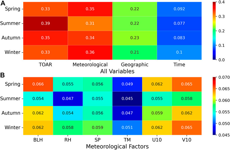
FIGURE 6. (A) The feature importance of all variables in different seasonal models, and (B) the feature importance of meteorological factors.

Among the various meteorological factors used in the model, U₁₀, V₁₀ and BLH contribute the most to the model, followed by RH, SP, and TM (Figure 6B). Wind speed can change the concentration of SO₂ by changing the diffusion and transport speed of SO₂, and BLH is related to the stability of the atmosphere and will directly affect the vertical mixing and long-distance diffusion of pollutants (Miao et al., 2018). Besides, some studies have shown that BLH can also have affect wind speed (Rigby and Toumi, 2008). In addition, the high RH environment can accelerate the heterogeneous absorption of SO₂ by aerosols, resulting in the conversion of SO₂ to sulfate (Zhang et al., 2015b; Wang et al., 2016; Fu and Chen, 2017). The SP and TM are related to the height of the boundary layer and the strength of the turbulence in the atmosphere (Zhang et al., 2015a; Mentes and Eper-Papai, 2015), which also affect the SO₂ concentration.

3.3 Spatial distribution of SO₂ in eastern China

By inputting the hourly data of each variable into the model, the hourly SO₂ concentration in eastern China is estimated, and then the spatial distribution of the mean value of SO₂ between 2016 and 2020 is calculated (Figure 7A). The result shows that the distribution of SO₂ concentrations has obvious regional differences, which are generally high in the north and low in the south (the average concentration in the north is 21.75 μg/m³, and the average concentration in the south is 18.05 μg/m³). The average concentration of SO₂ in North China is the highest, reaching 22.21 μg/m³. This is due to the existence of a large number of coal mining enterprises in these areas, coupled with the multivalley basin topography, resulting in a large accumulation of SO₂. The lowest annual concentration of SO₂ is found in the southeastern and northeastern regions of China. Compared with Figure 7B, it can be seen that the results predicted by the model are generally consistent with the observation.

FIGURE 7

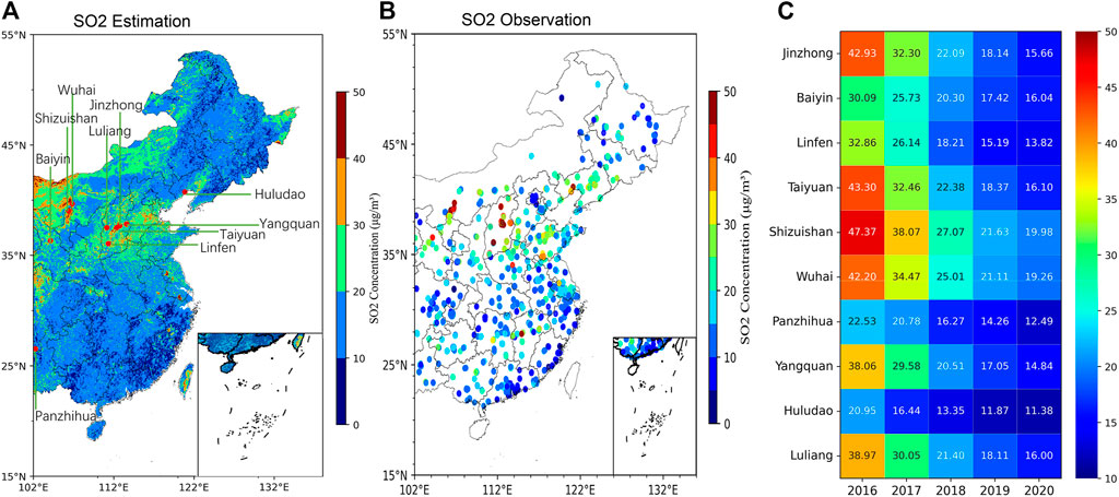
FIGURE 7. (A) The spatial distribution of the annual mean value of SO₂ between 2016 and 2020 predicted by the model (μg/m³), (B) the spatial distribution of the annual average SO₂ observation between 2016 and 2020 (μg/m³), and (C) the annual concentration changes predicted by the model of the 10 cities with the most serious SO₂ pollution (μg/m³).

Figure 7C shows the annual average SO₂ concentration predicted by the model of the 10 cities with the most serious SO₂ pollution in the ground monitoring data. There is a certain deviation between the predicted results of individual cities and the actual situation, but most cities are close to the actual situation. According to the results, the concentration of SO₂ in these cities gradually decreased from the high value in 2016 to less than 20 μg/m³ in 2020.

The mean values of SO₂ in spring, summer, autumn and winter from 2016 to 2020 are estimated, and their spatial distributions are shown in Figure 8. The results show that the concentration of SO₂ demonstrates obvious seasonal differences, and the concentration of SO₂ in winter is significantly higher than that in spring, summer and autumn, which is related to the large number of residents burning coal for heating in winter; furthermore, the stable atmospheric structure and low precipitation in winter are not conducive to wet deposition and diffusion of SO₂ (Calkins et al., 2016; Zhao et al., 2016). The concentration of SO₂ reaches the highest value in winter (25.88 μg/m³), then begins to decrease in spring (16.07 μg/m³), decreases to the lowest value in summer (14.22 μg/m³), and increases again in autumn (16.82 μg/m³). This phenomenon indicates that the concentration of SO₂ is continuous in the temporal scale.

FIGURE 8

FIGURE 8. Spatial distribution of the seasonal mean of SO₂ predicted by the model (μg/m³).

This study also estimates the hourly mean value of SO₂ between 9:00 and 16:00 in eastern China, and the results are shown in Figure 9. In general, the SO₂ concentration keeps declining between 9:00 and 16:00, with the highest concentration at 9:00 and the lowest at 16:00. The concentration in the morning is generally higher than that in the afternoon. This is because the temperature in the morning is lower than that in the afternoon, and the structure of the atmosphere is more stable, which is not conducive to SO₂ diffusion. The intraday variation of SO₂ concentration in southern China is not obvious, and SO₂ concentration maintains a low level throughout the day.

FIGURE 9

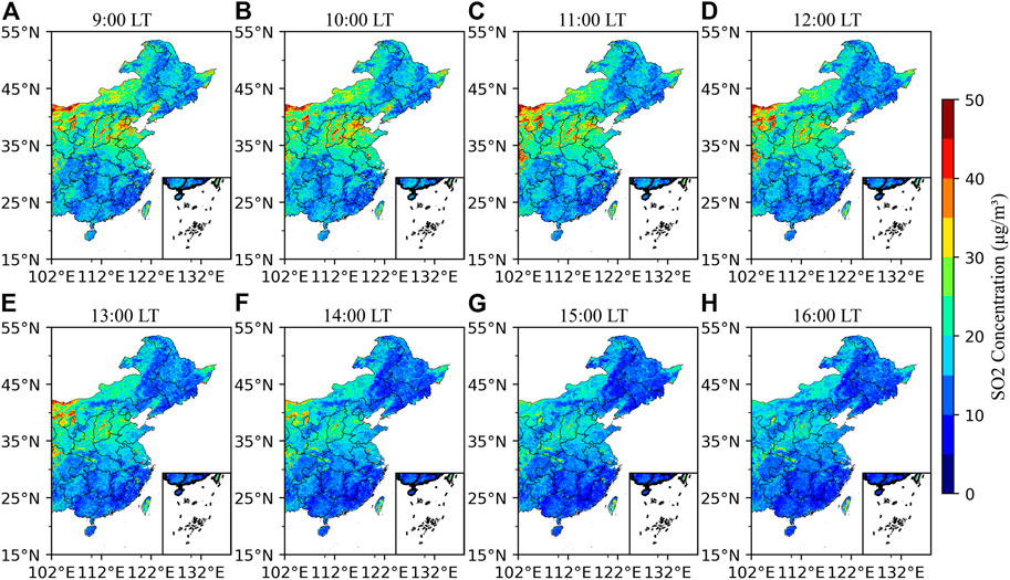
FIGURE 9. The intraday variation of SO₂ concentration predicted by the model (μg/m³).

Figure 10 shows the spatial distribution of the annual average concentration of SO₂ in North China (the specific location in Figure 1) estimated by the model from 2016 to 2020. In North China, the region with the most serious SO₂ pollution, the annual average concentration of SO₂ keeps declining from 2016 to 2020. In 2016, the SO₂ concentration exceeded 40 μg/m³ in many areas. In 2017, the SO₂ concentration decreased significantly, and the number of areas above 40 μg/m³ was greatly reduced. Within these areas, the SO₂ concentration decreased most in western Shanxi Province, western Hebei Province and central Inner Mongolia, but remained at a high level in northern Ningxia. In 2018, the SO₂ concentration further decreased, and only a few areas exceeded 40 μg/m³. By 2020, the SO₂ concentration in 90.52% of the North China was lower than the national ambient air quality SO₂ level 1 concentration limit of 20 μg/m³. In general, SO₂ pollution in North China has been effectively alleviated in the past 5 years, which is closely related to the wide application of flue gas desulfurization (Duan et al., 2016) and the government’s relevant policies to strengthen the control of SO₂ emissions such as coal desulfurization. In addition, SO₂ pollution levels have also been affected by the new coronavirus pneumonia epidemic (Fan et al., 2020; Ran et al., 2020).

FIGURE 10

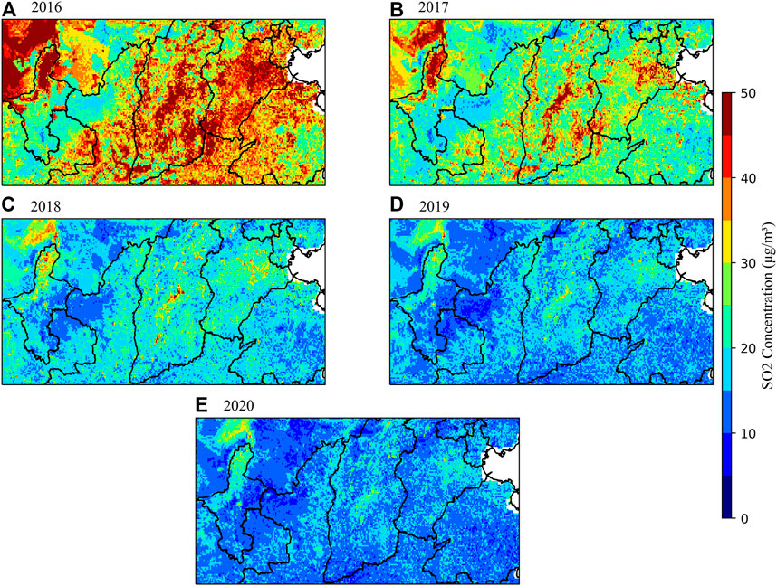
FIGURE 10. Spatial distribution of annual mean values of SO₂ in North China from 2016 to 2020 (μg/m³).

4 Discussion

In this study, we build a TOAR-SO₂ model with high spatial and temporal resolution over eastern China. The model performs well and can provide reliable SO₂ data for remote areas lacking ground monitoring stations, which is of great significance for SO₂ pollution control. The comparison of model performance between this study and other studies is shown in Table 5. In studies that cover a large area rather than just a city, the Space-Time Extra-Tree (STET) model (Wei et al., 2022) has the best effect, followed by our model. But our model has higher temporal and spatial resolution compared with the STET model. Figure 11 shows the comparison of annual average SO₂ concentrations in eastern China from 2016 to 2020 between the dataset estimated in this study and the ChinaHighSO₂ dataset estimated by the STET model. In general, the two have a good consistency, especially during 2018–2020. When estimating the annual average concentration of SO₂, the R² of ChinaHightSO₂ (0.98) is slightly higher than that in this study (0.97), but our RMSE (1.71 μg/m³) and MAE (0.82 μg/m³) are better than the RMAE (2.46 μg/m³) and MAE (1.35 μg/m³) of ChinaHightSO₂. Overall, both of these two models can be considered reliable in estimating the annual average SO₂ concentration.

TABLE 5

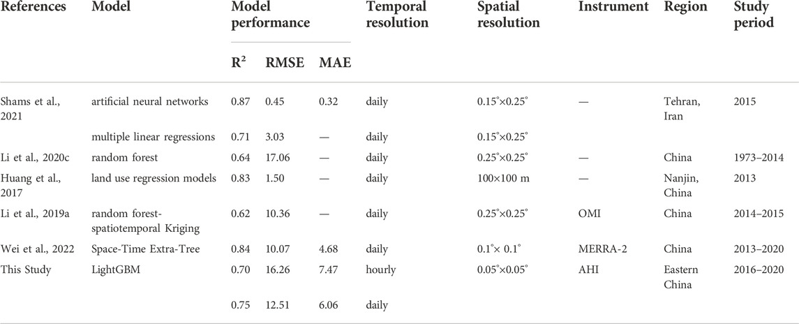
TABLE 5. Performance comparison of SO₂ model.

FIGURE 11

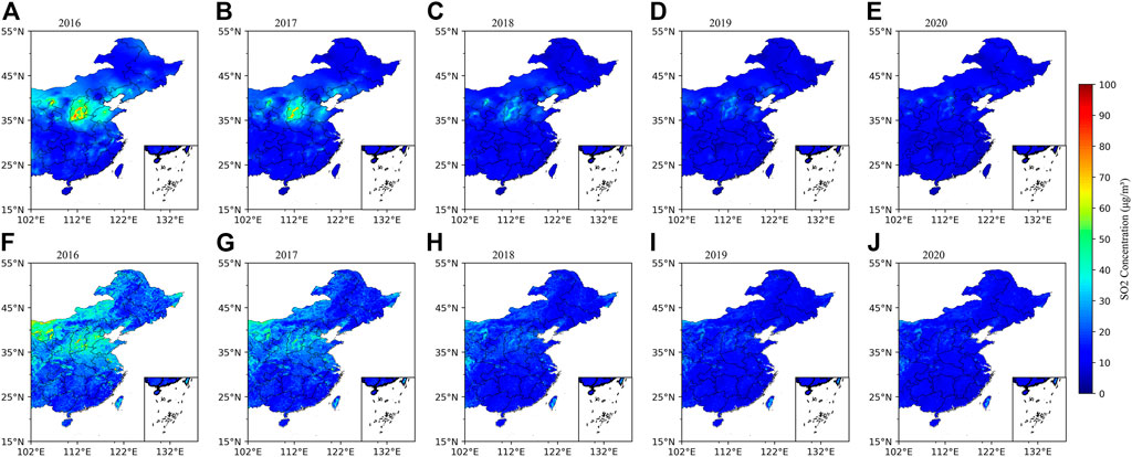
FIGURE 11. Comparison of annual average SO₂ concentrations in eastern China between our results and the ChinaHighSO₂. (A–E) the results of ChinaHighSO₂, and (F–J) the results of our study.

5 Conclusion

In this study, we apply Himawari-8 TOAR data to build a TOAR-SO₂ model with high spatial and temporal resolution based on the LightGBM machine learning model. The TOAR-SO₂ model can effectively capture high SO₂ events in winter, and works well when estimating monthly, seasonal, and annual average SO₂ with R² (RMSE) of 0.96 (2.75 μg/m³), 0.97 (2.16 μg/m³) and 0.97 (1.71 μg/m³). The concentration of SO₂ in North China estimated by the model showed a downward trend since 2016. Overall, the good agreement between ground measured and model estimated SO₂ concentrations highlights the capability and advantage of using the model to monitor spatiotemporal variations of SO₂ in Eastern China.

In the future, we need to improve the accuracy of the model in summer and extend the prediction range to the whole of China to obtain more accurate hourly concentrations of ground-level SO₂ with wider coverage. In addition, models established by machine learning methods lack interpretability. In the next step, we will improve the interpretability of the model by combining machine learning methods with the atmospheric chemistry model considering chemical mechanism.

Data availability statement

The estimated data and data reading codes are available from https://doi.org/10.5281/zenodo.7047543.

Author contributions

Conceptualization, BC; methodology, BC and TX; writing- original draft preparation, BC and TX; resources, BC; formal analysis, TX; software, TX, YR, LZ, XL, YW, JH, and ZS; data curation, TX, YR, LZ, XL, YW, JH, and ZS; visualization, TX and ZS. All authors have read and agreed to the published version of the manuscript.

Funding

The work was supported by the Second Tibetan Plateau Scientific Expedition and Research Program (STEP; Grant number 2019QZKK0602), the National Key Research and Development Program of China (Grant number 2019YFA0606800), and the Fundamental Research Funds for the Central Universities (Grant number lzujbky-2022-ct06).

Acknowledgments

The authors would like to thank China National Environmental Monitoring Center for the SO₂ ground observation data (http://www.cnemc.cn/en/); the Japan Meteorological Agency for the Himawari-8 TOAR data (http://www.eorc.jaxa.jp/ptree/index.html); European Centre for Medium-Range Weather Forecasts for the ERA-5 data (https://cds.climate.copernicus.eu/cdsapp#!/dataset/reanalysis-era5-land?tab=overview); and ChinaHighSO₂ dataset (https://doi.org/10.5281/zenodo.5765553).

Conflict of interest

The authors declare that the research was conducted in the absence of any commercial or financial relationships that could be construed as a potential conflict of interest.

Publisher’s note

All claims expressed in this article are solely those of the authors and do not necessarily represent those of their affiliated organizations, or those of the publisher, the editors and the reviewers. Any product that may be evaluated in this article, or claim that may be made by its manufacturer, is not guaranteed or endorsed by the publisher.

References

Calkins, C., Ge, C., Wang, J., Anderson, M., and Yang, K. (2016). Effects of meteorological conditions on sulfur dioxide air pollution in the North China plain during winters of 2006–2015. Atmos. Environ. 147, 296–309. doi:10.1016/j.atmosenv.2016.10.005

CrossRef Full Text | Google Scholar

Carn, S. A. (2005). Quantifying tropospheric volcanic emissions with AIRS: The 2002 eruption of Mt. Etna (Italy). Geophys. Res. Lett. 32 (2), L02301. doi:10.1029/2004gl021034

CrossRef Full Text | Google Scholar

Chen, B., Song, Z., Huang, J., Zhang, P., Hu, X., Zhang, X., et al. (2022a). Estimation of atmospheric PM10 concentration in China using an interpretable deep learning model and top-of-the-atmosphere reflectance data from China’s new generation geostationary meteorological satellite, FY-4A. JGR. Atmos. 127 (9). doi:10.1029/2021jd036393

CrossRef Full Text | Google Scholar

Chen, B., Song, Z., Pan, F., and Huang, Y. (2022b). Obtaining vertical distribution of PM2.5 from CALIOP data and machine learning algorithms. Sci. Total Environ. 805, 150338. doi:10.1016/j.scitotenv.2021.150338

PubMed Abstract | CrossRef Full Text | Google Scholar

Chen, B., Song, Z., Shi, B., and Li, M. (2022c). An interpretable deep forest model for estimating hourly PM10 concentration in China using Himawari-8 data. Atmos. Environ., 268, 118827, doi:10.1016/j.atmosenv.2021.118827

CrossRef Full Text | Google Scholar

Chen, Z. Y., Zhang, R., Zhang, T. H., Ou, C. Q., and Guo, Y. (2019). A kriging-calibrated machine learning method for estimating daily ground-level NO2 in mainland China. Sci. Total Environ. 690, 556–564. doi:10.1016/j.scitotenv.2019.06.349

PubMed Abstract | CrossRef Full Text | Google Scholar

Duan, L., Yu, Q., Zhang, Q., Wang, Z., Pan, Y., Larssen, T., et al. (2016). Acid deposition in Asia: Emissions, deposition, and ecosystem effects. Atmos. Environ. 146, 55–69. doi:10.1016/j.atmosenv.2016.07.018

CrossRef Full Text | Google Scholar

Eisinger, M., and Burrows, J. P. (1998). Tropospheric sulfur dioxide observed by the ERS-2 GOME instrument. Geophys. Res. Lett. 25 (22), 4177–4180. doi:10.1029/1998gl900128

CrossRef Full Text | Google Scholar

Fan, C., Li, Y., Guang, J., Li, Z., Elnashar, A., Allam, M., et al. (2020). The impact of the control measures during the COVID-19 outbreak on air pollution in China. Remote Sens. 12 (10), 1613. doi:10.3390/rs12101613

CrossRef Full Text | Google Scholar

Fu, H., and Chen, J. (2017). Formation, features and controlling strategies of severe haze-fog pollutions in China. Sci. Total Environ. 578, 121–138. doi:10.1016/j.scitotenv.2016.10.201

PubMed Abstract | CrossRef Full Text | Google Scholar

He, J., Gong, S., Yu, Y., Yu, L., Wu, L., Mao, H., et al. (2017). Air pollution characteristics and their relation to meteorological conditions during 2014-2015 in major Chinese cities. Environ. Pollut. 223, 484–496. doi:10.1016/j.envpol.2017.01.050

PubMed Abstract | CrossRef Full Text | Google Scholar

Hersbach, H., Bell, B., Berrisford, P., Hirahara, S., Horányi, A., Muñoz-Sabater, J., et al. (2020). The ERA5 global reanalysis. Q. J. R. Meteorol. Soc. 146 (730), 1999–2049. doi:10.1002/qj.3803

CrossRef Full Text | Google Scholar

Huang, L., Zhang, C., and Bi, J. (2017). Development of land use regression models for PM2.5, SO2, NO2 and O3 in Nanjing, China. Environ. Res. 158, 542–552. doi:10.1016/j.envres.2017.07.010

PubMed Abstract | CrossRef Full Text | Google Scholar

Ialongo, I., Herman, J., Krotkov, N., Lamsal, L., Boersma, K. F., Hovila, J., et al. (2016). Comparison of OMI NO<sub>2</sub> observations and their seasonal andweekly cycles with ground-based measurements in Helsinki. Atmos. Meas. Tech. 9 (10), 5203–5212. doi:10.5194/amt-9-5203-2016

CrossRef Full Text | Google Scholar

Johns, D. O., and Linn, W. S. (2011). A review of controlled human SO2 exposure studies contributing to the US EPA integrated science assessment for sulfur oxides. Inhal. Toxicol. 23 (1), 33–43. doi:10.3109/08958378.2010.539290

PubMed Abstract | CrossRef Full Text | Google Scholar

Ke, G., Meng, Q., Finley, T., Wang, T., Chen, W., Ma, W., et al. (2017). LightGBM: A highly efficient gradient boosting decision tree. California, USA: Curran Associates Inc, 3149–3157.

Google Scholar

Lee, A. K. (2015). Haze formation in China: Importance of secondary aerosol. J. Environ. Sci. 33, 261–262. doi:10.1016/j.jes.2015.06.002

PubMed Abstract | CrossRef Full Text | Google Scholar

Lee, C., Martin, R. V., Van Donkelaar, A., Lee, H., Dickerson, R. R., Hains, J. C., et al. (2011). SO2 emissions and lifetimes: Estimates from inverse modeling using in situ and global, space-based (SCIAMACHY and OMI) observations. J. Geophys. Res. 116 (6), D06304. doi:10.1029/2010jd014758

CrossRef Full Text | Google Scholar

Li, C., Krotkov, N. A., Carn, S., Zhang, Y., Spurr, R. J. D., and Joiner, J. (2017). New-generation NASA aura Ozone monitoring instrument (OMI) volcanic SO<sub>2</sub> dataset: Algorithm description, initial results, and continuation with the suomi-NPP Ozone mapping and profiler suite (OMPS). Atmos. Meas. Tech. 10 (2), 445–458. doi:10.5194/amt-10-445-2017

CrossRef Full Text | Google Scholar

Li, C., Krotkov, N. A., Leonard, P. J. T., Carn, S., Joiner, J., Spurr, R. J. D., et al. (2020a). Version 2 Ozone monitoring instrument SO<sub>2</sub> product (OMSO2 V2): New anthropogenic SO<sub>2</sub> vertical column density dataset. Atmos. Meas. Tech. 13 (11), 6175–6191. doi:10.5194/amt-13-6175-2020

CrossRef Full Text | Google Scholar

Li, F., Song, Z., and Liu, W. (2014). China's energy consumption under the global economic crisis: Decomposition and sectoral analysis. Energy Policy 64, 193–202. doi:10.1016/j.enpol.2013.09.014

CrossRef Full Text | Google Scholar

Li, H., Chen, R., Meng, X., Zhao, Z., Cai, J., Wang, C., et al. (2015). Short-term exposure to ambient air pollution and coronary heart disease mortality in 8 Chinese cities. Int. J. Cardiol. 197, 265–270. doi:10.1016/j.ijcard.2015.06.050

PubMed Abstract | CrossRef Full Text | Google Scholar

Li, R., Cui, L., Fu, H., Meng, Y., Li, J., and Guo, J. (2020b). Estimating high-resolution PM1 concentration from Himawari-8 combining extreme gradient boosting-geographically and temporally weighted regression (XGBoost-GTWR). Atmos. Environ. 229, 117434. doi:10.1016/j.atmosenv.2020.117434

CrossRef Full Text | Google Scholar

Li, R., Cui, L., Liang, J., Zhao, Y., Zhang, Z., and Fu, H. (2020c). Estimating historical SO2 level across the whole China during 1973-2014 using random forest model. Chemosphere 247, 125839. doi:10.1016/j.chemosphere.2020.125839

PubMed Abstract | CrossRef Full Text | Google Scholar

Li, R., Cui, L., Meng, Y., Zhao, Y., and Fu, H. (2019a). Satellite-based prediction of daily SO2 exposure across China using a high-quality random forest-spatiotemporal Kriging (RF-STK) model for health risk assessment. Atmos. Environ. 208, 10–19. doi:10.1016/j.atmosenv.2019.03.029

CrossRef Full Text | Google Scholar

Li, R., Fu, H., Cui, L., Li, J., Wu, Y., Meng, Y., et al. (2019b). The spatiotemporal variation and key factors of SO2 in 336 cities across China J. Clean. Prod. 210, 602–611. doi:10.1016/jclepro.2018.11.062

CrossRef Full Text | Google Scholar

Liu, F., Zhang, Q., Van Der, A. R. J., Zheng, B., Tong, D., Yan, L., et al. (2016). Recent reduction in NO emissions over China: Synthesis of satellite observations and emission inventories. Environ. Res. Lett. 11 (11), 114002. doi:10.1088/1748-9326/11/11/114002

CrossRef Full Text | Google Scholar

Liu, T., Gong, S., He, J., Yu, M., Wang, Q., Li, H., et al. (2017). Attributions of meteorological and emission factors to the 2015 winter severe haze pollution episodes in China's Jing-Jin-Ji area. Atmos. Chem. Phys. 17 (4), 2971–2980. doi:10.5194/acp-17-2971-2017

CrossRef Full Text | Google Scholar

Ma, J., Zhang, R., Xu, J., and Yu, Z. (2022). MERRA-2 PM2.5 mass concentration reconstruction in China mainland based on LightGBM machine learning. Sci. Total Environ. 827, 154363. doi:10.1016/j.scitotenv.2022.154363

PubMed Abstract | CrossRef Full Text | Google Scholar

Mentes, G., and Eper-Papai, I. (2015). Investigation of temperature and barometric pressure variation effects on radon concentration in the Sopronbanfalva Geodynamic Observatory, Hungary. J. Environ. Radioact. 149, 64–72. doi:10.1016/j.jenvrad.2015.07.015

PubMed Abstract | CrossRef Full Text | Google Scholar

Miao, Y., Liu, S., Guo, J., Huang, S., Yan, Y., and Lou, M. (2018). Unraveling the relationships between boundary layer height and PM2.5 pollution in China based on four-year radiosonde measurements. Environ. Pollut. 243 (B), 1186–1195. doi:10.1016/j.envpol.2018.09.070

PubMed Abstract | CrossRef Full Text | Google Scholar

Ran, J., Zhao, S., Han, L., Peng, Z., Wang, M. H., Qiu, Y., et al. (2020). Initial COVID-19 transmissibility and three gaseous air pollutants (NO2, SO2, and CO): A nationwide ecological study in China. Front. Med. 7, 575839. doi:10.3389/fmed.2020.575839

CrossRef Full Text | Google Scholar

Rigby, M., and Toumi, R. (2008). London air pollution climatology: Indirect evidence for urban boundary layer height and wind speed enhancement. Atmos. Environ. 42 (20), 4932–4947. doi:10.1016/j.atmosenv.2008.02.031

CrossRef Full Text | Google Scholar

Shams, S. R., Jahani, A., Kalantary, S., Moeinaddini, M., and Khorasani, N. (2021). The evaluation on artificial neural networks (ANN) and multiple linear regressions (MLR) models for predicting SO2 concentration. Urban Clim. 37, 100837. doi:10.1016/j.uclim.2021.100837

CrossRef Full Text | Google Scholar

Song, Y., Wang, X., Maher, B. A., Li, F., Xu, C., Liu, X., et al. (2016). The spatial-temporal characteristics and health impacts of ambient fine particulate matter in China. J. Clean. Prod. 112, 1312–1318. doi:10.1016/j.jclepro.2015.05.006

CrossRef Full Text | Google Scholar

Song, Z., Chen, B., and Huang, J. (2022a). Combining Himawari-8 AOD and deep forest model to obtain city-level distribution of PM2.5 in China. Environ. Pollut. 297, 118826. doi:10.1016/j.envpol.2022.118826

PubMed Abstract | CrossRef Full Text | Google Scholar

Song, Z., Chen, B., Zhang, P., Guan, X., Wang, X., Ge, J., et al. (2022b). High temporal and spatial resolution PM2.5 dataset acquisition and pollution assessment based on FY-4A TOAR data and deep forest model in China. Atmos. Res. 274, 106199. doi:10.1016/j.atmosres.2022.106199

CrossRef Full Text | Google Scholar

Sunyer, J. (2003). The association of daily sulfur dioxide air pollution levels with hospital admissions for cardiovascular diseases in Europe (The Aphea-II study). Eur. Heart J. 24 (8), 752–760. doi:10.1016/s0195-668x(02)00808-4

PubMed Abstract | CrossRef Full Text | Google Scholar

Tripathy, A., Vaidya, D., Mishra, A., Bilolikar, S., and Thoday, V. (2021). Analysing and predicting air quality in Delhi: Comparison of industrial and residential area. Air Device, 1–6.

CrossRef Full Text | Google Scholar

Wang, G., Zhang, R., Gomez, M. E., Yang, L., Levy Zamora, M., Hu, M., et al. (2016). Persistent sulfate formation from London Fog to Chinese haze. Proc. Natl. Acad. Sci. U. S. A. 113 (48), 13630–13635. doi:10.1073/pnas.1616540113

PubMed Abstract | CrossRef Full Text | Google Scholar

Wang, L., Liu, C., Meng, X., Niu, Y., Lin, Z., Liu, Y., et al. (2018). Associations between short-term exposure to ambient sulfur dioxide and increased cause-specific mortality in 272 Chinese cities. Environ. Int. 117, 33–39. doi:10.1016/j.envint.2018.04.019

PubMed Abstract | CrossRef Full Text | Google Scholar

Wei, J., Huang, W., Li, Z., Xue, W., Peng, Y., Sun, L., et al. (2019). Estimating 1-km-resolution PM2.5 concentrations across China using the space-time random forest approach. Remote Sens. Environ. 231, 111221. doi:10.1016/j.rse.2019.111221

CrossRef Full Text | Google Scholar

Wei, J., Li, Z., Pinker, R. T., Wang, J., Sun, L., Xue, W., et al. (2021). Himawari-8-derived diurnal variations in ground-level PM<sub>2.5</sub> pollution across China using the fast space-time Light Gradient Boosting Machine (LightGBM). Atmos. Chem. Phys. 21 (10), 7863–7880. doi:10.5194/acp-21-7863-2021

CrossRef Full Text | Google Scholar

Wei, J., Li, Z., Wang, J., Li, C., Gupta, P., and Cribb, M. (2022). Atmosphere pressure. High 25, 366.

Google Scholar

Xie, Y., Zhao, B., Zhang, L., and Luo, R. (2015). Spatiotemporal variations of PM2.5 and PM10 concentrations between 31 Chinese cities and their relationships with SO2, NO2, CO and O3. Particuology 20, 141–149. doi:10.1016/j.partic.2015.01.003

CrossRef Full Text | Google Scholar

Xu, Q., Chen, X., Yang, S., Tang, L., and Dong, J. (2021). Spatiotemporal relationship between Himawari-8 hourly columnar aerosol optical depth (AOD) and ground-level PM2.5 mass concentration in mainland China. Sci. Total Environ. 765, 144241. doi:10.1016/j.scitotenv.2020.144241

PubMed Abstract | CrossRef Full Text | Google Scholar

Yang, K., Krotkov, N. A., Krueger, A. J., Carn, S. A., Bhartia, P. K., and Levelt, P. F. (2007). Retrieval of large volcanic SO2columns from the aura Ozone monitoring instrument: Comparison and limitations. J. Geophys. Res. 112 (D24), D24S43. doi:10.1029/2007jd008825

CrossRef Full Text | Google Scholar

Yoshida, M., Kikuchi, M., Nagao, T. M., Murakami, H., Nomaki, T., and Higurashi, A. (2018). Common retrieval of aerosol properties for imaging satellite sensors. J. Meteorological Soc. Jpn. 96B (0), 193–209. doi:10.2151/jmsj.2018-039

CrossRef Full Text | Google Scholar

Yu, T., Wang, W., Ciren, P., and Sun, R. (2018). An assessment of air-quality monitoring station locations based on satellite observations. Int. J. Remote Sens. 39 (20), 6463–6478. doi:10.1080/01431161.2018.1460505

CrossRef Full Text | Google Scholar

Zang, L., Mao, F., Guo, J., Gong, W., Wang, W., and Pan, Z. (2018). Estimating hourly PM1 concentrations from Himawari-8 aerosol optical depth in China. Environ. Pollut. 241, 654–663. doi:10.1016/j.envpol.2018.05.100

PubMed Abstract | CrossRef Full Text | Google Scholar

Zang, L., Mao, F., Guo, J., Wang, W., Pan, Z., Shen, H., et al. (2019). Estimation of spatiotemporal PM1.0 distributions in China by combining PM2.5 observations with satellite aerosol optical depth. Sci. Total Environ. 658, 1256–1264. doi:10.1016/j.scitotenv.2018.12.297

PubMed Abstract | CrossRef Full Text | Google Scholar

Zhang, H., Wang, Y., Hu, J., Ying, Q., and Hu, X. M. (2015a). Relationships between meteorological parameters and criteria air pollutants in three megacities in China. Environ. Res. 140, 242–254. doi:10.1016/j.envres.2015.04.004

PubMed Abstract | CrossRef Full Text | Google Scholar

Zhang, L., Lee, C. S., Zhang, R., and Chen, L. (2017). Spatial and temporal evaluation of long term trend (2005–2014) of OMI retrieved NO2 and SO2 concentrations in Henan Province, China. Atmos. Environ. 154, 151–166. doi:10.1016/j.atmosenv.2016.11.067

CrossRef Full Text | Google Scholar

Zhang, Y., Li, Z., Cuesta, J., Li, D., Wei, P., Xie, Y., et al. (2015b). Aerosol column size distribution and water uptake observed during a major haze outbreak over beijing on january 2013. Aerosol Air Qual. Res. 15 (3), 945–957. doi:10.4209/aaqr.2014.05.0099

CrossRef Full Text | Google Scholar

Zhao, S., Yu, Y., Yin, D., He, J., Liu, N., Qu, J., et al. (2016). Annual and diurnal variations of gaseous and particulate pollutants in 31 provincial capital cities based on in situ air quality monitoring data from China National Environmental Monitoring Center. Environ. Int. 86, 92–106. doi:10.1016/j.envint.2015.11.003

PubMed Abstract | CrossRef Full Text | Google Scholar

Zhu, T., Shang, J., and Zhao, D. (2011). The roles of heterogeneous chemical processes in the formation of an air pollution complex and gray haze. Sci. China Chem. 54 (1), 145–153. doi:10.1007/s11426-010-4181-y

CrossRef Full Text | Google Scholar