Constrained shuffled complex evolution algorithm and its application in the automatic calibration of Xinanjiang model

The Shuffled Complex Evolution—University of Arizona (SCE-UA) is a classical algorithm in the field of hydrology and water resources, but it cannot solve constrained optimization problems directly. Using penalty functions has been the preferred method to handle constraints, but the appropriate selection of penalty parameters and penalty functions can be challenging. To enhance the universality of the SCE-UA, we propose the Constrained Shuffled Complex Evolution Algorithm (CSCE) to conveniently and effectively solve inequality-constrained optimization problems. Its performance is compared with the SCE-UA using the adaptive penalty function (SCEA) on 14 test problems with inequality constraints. It is further compared with seven other algorithms on two test problems with low success rates. To demonstrate its effect in hydrologic model calibration, the CSCE is applied to the parameter optimization of the Xinanjiang (XAJ) model under synthetic data and observed data. The results indicate that the CSCE is more advantageous than the SCEA in terms of the success rate, stability, feasible rate, and convergence speed. It can guarantee the feasibility of the solution and avoid the problem of deep soil tension water capacity (WDM)<0 in the optimization process of the XAJ model. In the case of synthetic data, the CSCE can accurately find the theoretical optimal parameters of the XAJ model under the given constraints. In the case of observed data, the XAJ model optimized by the CSCE can effectively simulate the hourly rainfall-runoff events of the Hexi Basin and achieves mean Nash efficiency coefficients greater than 0.75 in the calibration period and the validation period.

1 Introduction

The Shuffled Complex Evolution algorithm (SCE-UA) was proposed by the University of Arizona (Duan et al., 1993). It offers a global search strategy by the synthesis of the down-hill simplex method (Nelder and Mead, 1965), clustering, competitive evolution, complex shuffling, and so on. Since its invention, the SCE-UA has been widely used in the automatic calibration of hydrologic models such as the Sacramento model (Ajami et al., 2004), the Tank model (Cooper et al., 1997), and the Xinanjiang (XAJ) model (Jayawardena et al., 2006). In addition, it has been applied in other domains such as the optimal allocation of water resources (Ayad et al., 2021), optimal reservoir operation (Le Ngo et al., 2007), and groundwater management (Ketabchi and Ataie-Ashtiani, 2015). Over the past 30 years, the SCE-UA has undergone many improvements and has derived many improved versions, such as the SCEM-UA (Vrugt et al., 2003b) for uncertainty assessment, the MOCOM-UA (Yapo et al., 1998) and MOSCEM (Vrugt et al., 2003a) for solving multi-objective optimization problems. Previous research mainly focused on improving search capability, multi-objective optimization, and uncertainty assessment, but studies on the application of the SCE-UA under constraints are still limited (Naeini et al., 2019).

Many problems in the field of hydrology and water resources can be generalized to constrained nonlinear optimization problems. For example, in the field of hydrologic model calibration, it is sometimes necessary to add inequality constraints between parameters to obtain optimization results that conform to the physical meaning of parameters. In the field of reservoir operation, there are constraints on the reservoir water level, water balance, and flood discharge. However, the SCE-UA cannot directly solve constrained optimization problems because its default feasible region is a multidimensional space composed of the upper and lower boundaries of each parameter. Using penalty function is a simple and efficient way to handle constraints, it converts a constrained optimization problem to an unconstrained one (Askarzadeh, 2016; Gupta et al., 2017). In the field of water resources, many studies have used penalty functions to address the constraints of groundwater management (Eusuff and Lansey, 2004) and reservoir operation (Chang et al., 2010). The static penalty function is the simplest method. In this method, the penalty value is added to the objective function so that the infeasible individual will be penalized for violating the constraints. However, the penalty parameter and the penalty function are difficult to configure subjectively (Deb, 2000), they are problem-dependent. Adaptive penalty functions have been developed to overcome the drawbacks of static penalty functions (Farmani and Wright, 2003). They have been applied to constrained optimization problems in earth science such as seismic inversion (Guo et al., 2021). Adaptive penalty functions do not require users to adjust the penalty parameters in advance. However, there are still infeasible points involved in the calculation of the objective function, and the result may also be an infeasible solution. In addition, if the objective function value cannot be calculated at the infeasible points, this method is invalid. Lee and Kang (2016) combined the adaptive penalty function proposed by Tessema and Yen (2009) with the SCE-UA algorithm (hereinafter referred to as SCEA) and applied it to the calibration of the stormwater management model (SWMM) (Kang and Lee, 2014). However, the SCEA was tested only on two two-dimensional test functions in their paper and it has not been compared with other algorithms yet.

The constrained shuffled complex evolution algorithm (CSCE) we developed aims to solve inequality-constrained optimization problems more efficiently and conveniently. Its structural design ensures that all its solutions are feasible. As with the adaptive penalty function, the CSCE has no new parameters to be adjusted before optimization. Later in this paper, the CSCE is tested on 14 problems and compared with the SCEA. Then, it is applied to the calibration of the XAJ model.

2 Algorithms

2.1 The SCE-UA

The main parameters of the SCE-UA are the dimension of the problem n and the number of complexes p. The recommended values (Duan et al., 1994) for other parameters are as follows: the number of points in each complex m=2n+1, the number of points in each subcomplex q=n+1, the number of times each complex is adjusted β=2n+1, and the number of times each subcomplex is adjusted α=1. Therefore, the number of complexes p determines the size of the initial population (s=mp), and it can be set according to the complexity of the optimization problem. The main steps of the SCE-UA are as follows:

Step 1:. Randomly initialize s sample points (s=mp) in the feasible region, and calculate their objective function values.

Step 2:. Sort the sample points in ascending order by objective function values.

Step 3:. Divide the s sorted points into p complexes, and each complex contains m points.

Step 4:. Evolve each complex β times with the competitive complex evolution (CCE) algorithm. In each evolution, q points in a complex are selected to form a subcomplex, and the subcomplex is adjusted α times using reflection, contraction, and mutation steps.

Step 5:. Mix all points in the evolved complexes and sort them in ascending order of objective function value.

Step 6:. Determine whether the termination criteria are met, if not, return to Step 3.The SCE-UA is popular mainly due to the following reasons: The algorithm is easy to understand and be implemented by programming; Many parts of the algorithm such as the initialization of complexes and the evolution of complexes are parallelizable, which is suitable for parallel computing when optimizing large and complex problems (Kan et al., 2016); Only the number of complexes p needs to be adjusted by users when using the recommended values of other parameters (Duan et al., 1994), and these recommendations have stood the test of time; The algorithm has proven to be more efficient and robust than some classic algorithms such as the genetic algorithm (GA), the simulated annealing algorithm (SAA), and the differential evolution algorithm (DE) in solving some problems in the field of hydrology and water resources by some researches (Cooper et al., 1997; Arsenault et al., 2014). For detailed information about the SCE-UA, please refer to the original paper (Duan et al., 1993).

2.2 The SCEA

The adaptive penalty function in the SCEA was proposed by Tessema and Yen (2009). It can adjust the penalty coefficient adaptively by using the feasible ratio in the current population (the proportion of the feasible individuals in the population) to control the intensity of the penalty. It was initially embedded in genetic algorithms to solve constrained optimization problems, and achieved good results on 22 benchmark functions. Lee and Kang (2016) embedded this adaptive penalty function into the SCE-UA and proposed the SCEA.

Optimization problems with inequality constraints can usually be expressed as:

$\begin{array}{c}\mathbf{M}\mathbf{i}\mathbf{n}\mathbf{i}\mathbf{m}\mathbf{i}\mathbf{z}\mathbf{e}\mathbf{f}\left(\overrightarrow{\mathbf{x}}\right)\\ \mathbf{s}\mathbf{u}\mathbf{b}\mathbf{j}\mathbf{e}\mathbf{c}\mathbf{t}\mathbf{t}\mathbf{o}\{\begin{array}{c}{\mathbf{g}}_{\mathbf{j}}\left(\overrightarrow{\mathbf{x}}\right)\le 0,\mathbf{j}=\mathbf{1},\dots ,\mathbf{m}\\ \overrightarrow{\mathbf{x}}\in \mathbf{X}\end{array}\end{array}(1)$

where n is the number of decision variables, $\overrightarrow{\mathbf{x}}=\left({\mathrm{x}}_1,{\mathrm{x}}_2,\dots ,{\mathrm{x}}_{\mathrm{n}}\right)$; m is the number of inequality constraints; and X is the search space composed of the upper and lower boundaries of each decision variable. The region in X that satisfies all inequality constraints is the feasible region Ω.

The objective function of all current points will be evaluated first, and each point’s function value will be normalized by the following formula:

$\begin{array}{c}\stackrel{\sim }{\mathbf{f}}\left(\overrightarrow{\mathbf{x}}\right)=\frac{\mathbf{f}\left(\overrightarrow{\mathbf{x}}\right)-{\mathbf{f}}_{\mathbf{min}}}{{\mathbf{f}}_{\mathbf{max}}{-\mathbf{f}}_{\mathbf{min}}}\end{array}(2)$

where $\stackrel{\sim }{\mathrm{f}}\left(\overrightarrow{\mathrm{x}}\right)$ is the normalized objective function value; $\mathrm{f}\left(\overrightarrow{\mathrm{x}}\right)$ is the original objective function value; ${\mathrm{f}}_{\max }$ and ${\mathrm{f}}_{\min }$ are the maximum and minimum values of the objective function in the current population respectively. The violation of each infeasible point is calculated by the following formula:

$\begin{array}{c}\mathbf{v}\left(\overrightarrow{\mathbf{x}}\right)=\frac{\mathbf{1}}{\mathbf{m}}{\displaystyle \sum }_{\mathbf{j}=\mathbf{1}}^{\mathbf{m}}\frac{{\mathbf{c}}_{\mathbf{j}}\left(\overrightarrow{\mathbf{x}}\right)}{{\mathbf{c}}_{\mathbf{max},\mathbf{j}}}\end{array}(3)$

$\begin{array}{c}{\mathbf{c}}_{\mathbf{j}}\left(\overrightarrow{\mathbf{x}}\right)=\mathbf{max}\left\{\mathbf{0},{\mathbf{g}}_{\mathbf{j}}\left(\overrightarrow{\mathbf{x}}\right)\right\},\mathbf{j}=\mathbf{1},\dots ,\mathbf{m}\end{array}(4)$

where ${\mathrm{c}}_{\mathrm{j}}\left(\overrightarrow{\mathrm{x}}\right)$ is the violation of the point $\overrightarrow{\mathrm{x}}$ for constraint j; $\mathrm{v}\left(\overrightarrow{\mathrm{x}}\right)$ is the violation of the point $\overrightarrow{\mathrm{x}}$ for all constraints; ${\mathrm{c}}_{\max ,\mathrm{j}}$ is the maximum value of ${\mathrm{c}}_{\mathrm{j}}\left(\overrightarrow{\mathrm{x}}\right)$ in the current population. Then, the modified objective function value is calculated by the following formula:

$\begin{array}{c}\mathbf{F}\left(\overrightarrow{\mathbf{x}}\right)=\{\begin{array}{cc}\stackrel{\sim }{\mathbf{f}}\left(\overrightarrow{\mathbf{x}}\right),& \mathbf{r}>\mathbf{0}\mathbf{a}\mathbf{n}\mathbf{d}\overrightarrow{\mathbf{x}}\mathbf{i}\mathbf{s}\mathbf{f}\mathbf{e}\mathbf{a}\mathbf{s}\mathbf{i}\mathbf{b}\mathbf{l}\mathbf{e}\\ \mathbf{v}\left(\overrightarrow{\mathbf{x}}\right),& \mathbf{r}=\mathbf{0}\\ \sqrt{{\stackrel{\sim }{\mathbf{f}}\left(\overrightarrow{\mathbf{x}}\right)}^{\mathbf{2}}{+\mathbf{v}\left(\overrightarrow{\mathbf{x}}\right)}^{\mathbf{2}}}+\left[\left(\mathbf{1}-\mathbf{r}\right)\mathbf{v}\left(\overrightarrow{\mathbf{x}}\right)+\mathbf{r}\stackrel{\sim }{\mathbf{f}}\left(\overrightarrow{\mathbf{x}}\right)\right],& \mathbf{r}>\mathbf{0}\mathbf{a}\mathbf{n}\mathbf{d}\overrightarrow{\mathbf{x}}\mathbf{i}\mathbf{s}\mathbf{i}\mathbf{n}\mathbf{f}\mathbf{e}\mathbf{a}\mathbf{s}\mathbf{i}\mathbf{b}\mathbf{l}\mathbf{e}\end{array}\end{array}(5)$

$\begin{array}{c}\mathrm{r}=\frac{\mathrm{n}\mathrm{u}\mathrm{m}\mathrm{b}\mathrm{e}\mathrm{r}\mathrm{o}\mathrm{f}\mathrm{f}\mathrm{e}\mathrm{a}\mathrm{s}\mathrm{i}\mathrm{b}\mathrm{l}\mathrm{e}\mathrm{p}\mathrm{o}\mathrm{i}\mathrm{n}\mathrm{t}\mathrm{s}\mathrm{i}\mathrm{n}\mathrm{t}\mathrm{h}\mathrm{e}\mathrm{c}\mathrm{u}\mathrm{r}\mathrm{r}\mathrm{e}\mathrm{n}\mathrm{t}\mathrm{p}\mathrm{o}\mathrm{p}\mathrm{u}\mathrm{l}\mathrm{a}\mathrm{t}\mathrm{i}\mathrm{o}\mathrm{n}}{\mathrm{p}\mathrm{o}\mathrm{p}\mathrm{u}\mathrm{l}\mathrm{a}\mathrm{t}\mathrm{i}\mathrm{o}\mathrm{n}\mathrm{s}\mathrm{i}\mathrm{z}\mathrm{e}}\end{array}(6)$

where r is the ratio of feasible points in the current population; $\mathrm{F}\left(\overrightarrow{\mathrm{x}}\right)$ is the modified objective function. If there is no feasible point (r=0) in the current population, the original objective function value will be disregarded, and $\mathrm{F}\left(\overrightarrow{\mathrm{x}}\right)$ is equal to the violation of point $\overrightarrow{\mathrm{x}}$. This helps to find feasible points first before searching for the optimum value. If there are feasible points in the current population (r>0), $\mathrm{F}\left(\overrightarrow{\mathrm{x}}\right)$ is equal to the normalized objective function value for feasible points, and for infeasible points, $\mathrm{F}\left(\overrightarrow{\mathrm{x}}\right)$ is determined by the violation, the normalized objective function value, and the feasibility ratio. Then, the adaptive penalty function method is embedded into the SCE-UA in the form of a subroutine (Figure 1).

FIGURE 1

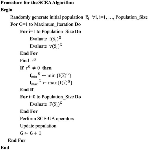
FIGURE 1. Pseudocode of the SCEA.

2.3 The CSCE

The SCE-UA has two parts for generating and updating points: 1. the generation of initial points. 2. the competitive complex evolution (CCE) algorithm. Therefore, the above two parts were modified to ensure that all new points were in the feasible region. Meanwhile, the improved simplex search method proposed by Muttil and Jayawardena (2008) was introduced to enhance search efficiency. The remaining steps of the CSCE are the same as those of the SCE-UA.

2.3.1 Strategy for generating initial feasible points

X is the space composed of the upper and lower boundaries of each decision variable. The task of the initial feasible point search is to search space X to find a point in the feasible region Ω. For many real-world problems, the feasible region is usually not very small, random searching by computer is sufficient to find the initial feasible point, using a complex algorithm increases the running time of the program instead. However, for problems with high dimensions and complex constraints, this method will become time-consuming. Therefore, quickly and efficiently finding the initial feasible points that satisfy the constraints is a difficult problem in the field of optimization. We used a strategy similar to the univariate search technique (Liu et al., 2001) to generate the initial feasible points. $\overrightarrow{\mathrm{x}}=\left({\mathrm{x}}_1,{\mathrm{x}}_2,\dots ,{\mathrm{x}}_{\mathrm{n}}\right)$ is a vector of decision variables; $\overrightarrow{\mathrm{a}}=\left({\mathrm{a}}_1,{\mathrm{a}}_2,\dots ,{\mathrm{a}}_{\mathrm{n}}\right)$ and $\overrightarrow{\mathrm{b}}=\left({\mathrm{b}}_1,{\mathrm{b}}_2,\dots ,{\mathrm{b}}_{\mathrm{n}}\right)$ represent the lower and upper boundaries of each variable respectively; S represents how many constraints $\overrightarrow{\mathrm{x}}$ can satisfy, and it is the guidance of searching, the point meeting more constraints will be retained as a new basic point for searching to approach the feasible region. If $\overrightarrow{\mathrm{x}}$ is feasible, S=m; Q is the maximum number of adjustments in each dimension, and its default value is 10; L is the maximum number of adjustments based on a starting point, and the default value is four; and $\overrightarrow{\mathrm{Y}}=\left({\mathrm{y}}_1,{\mathrm{y}}_2,\dots ,{\mathrm{y}}_{\mathrm{n}}\right)$ is the retention point. Q and L only affect the search time, and they can be adjusted by users according to specific problems if necessary. Here we use their default values. The search steps are as follows:

Step 1: Randomly generate a starting point $\overrightarrow{{\mathrm{x}}_0}$ in space X, calculate S, and let ${\mathrm{S}}_1=\mathrm{S}$ and $\overrightarrow{\mathrm{Y}}=\overrightarrow{{\mathrm{x}}_0}$. If S1=m, find the feasible point, output $\overrightarrow{\mathrm{Y}}$, and stop the algorithm; otherwise, go to step 2.

Step 2: Adjust based on $\overrightarrow{\mathrm{Y}}$. Fix ${\mathrm{x}}_2,\dots ,{\mathrm{x}}_{\mathrm{n}}$, and adjust $\overrightarrow{\mathrm{Y}}$ in the ${\mathrm{x}}_1$-axis direction. $\overrightarrow{{\mathrm{e}}_1}=\left(\mathrm{1,0,0},\dots ,0\right),$ randomly generate ${\mathrm{x}}_1$ in the interval ${[\mathrm{a}}_1,{\mathrm{b}}_1]$, new point $\overrightarrow{{\mathrm{x}}_1}=\overrightarrow{\mathrm{Y}}+\left({\mathrm{x}}_1-{\mathrm{y}}_1\right)\overrightarrow{{\mathrm{e}}_1}$, calculate S.

(a) If S=m, find the feasible point, output $\overrightarrow{{\mathrm{x}}_1}$ , and stop the algorithm.

(b) If ${\mathrm{S}}_1<\mathrm{S}<\mathrm{m}$, find the better point, set ${\mathrm{S}}_1=\mathrm{S}$, and set $\overrightarrow{\mathrm{Y}}=\overrightarrow{{\mathrm{x}}_1}$. Go to step 3.

(c) If $\mathrm{S}\le {\mathrm{S}}_1$, return to step 2. If no feasible point or better point is found after Q adjustments in the ${\mathrm{x}}_1$-axis direction, go to step 3.

Step 3: Perform operations similar to step 2 in the ${\mathrm{x}}_2,\dots ,{\mathrm{x}}_{\mathrm{n}}$ axis directions in turn completing a round of adjustment. If no feasible point is found, return to step 2 and start a new round of adjustment. If no feasible point is found after L rounds of adjustment, return to step 1, regenerate a new starting point $\overrightarrow{{\mathrm{x}}_0}$ and repeat until a feasible point is found.By performing the above algorithm s times, s initial feasible points are generated. Figure 2 shows the flow chart of this search strategy.To show the effect of this method, 30 points meeting the following constraints were generated. They are the constraints of the subsequent test problem G07 in this paper, and the feasible region is only 0.0003% of the search space. The experiment was done on the Windows operating system and Pycharm 2021.2.1. The search strategy uses 25s to find all feasible points while it takes 1136s to randomly generate all feasible points by computer.

$\begin{array}{c}\mathrm{S}\mathrm{u}\mathrm{b}\mathrm{j}\mathrm{e}\mathrm{c}\mathrm{t}\mathrm{t}\mathrm{o}\{\begin{array}{c}-105+4x_1+5x_2-3x_7+9x_8\le 0\\ 10x_1-8x_2-17x_7+2x_8\le 0\\ -8x_1+2x_2+5x_9-2x_{10}-12\le 0\\ 3{\left(x_1-2\right)}^2+4{\left(x_2-3\right)}^2+2x_3^2-7x_4-120\le 0\\ 5x_1^2+8x_2+{\left(x_3-6\right)}^2-2x_4-40\le 0\\ x_1^2+2{\left(x_2-2\right)}^2-2x_1{x}_2+14x_5-6x_6\le 0\\ 0.5{\left(x_1-8\right)}^2+2{\left(x_2-4\right)}^2+3x_5^2-x_6-30\le 0\\ -3x_1+6x_2+12{\left(x_9-8\right)}^2-7x_{10}\le 0\\ {-10\le x}_i\le 10,i=\mathrm{1,2},\dots ,10\\ \\ \end{array}\end{array}(7)$

FIGURE 2

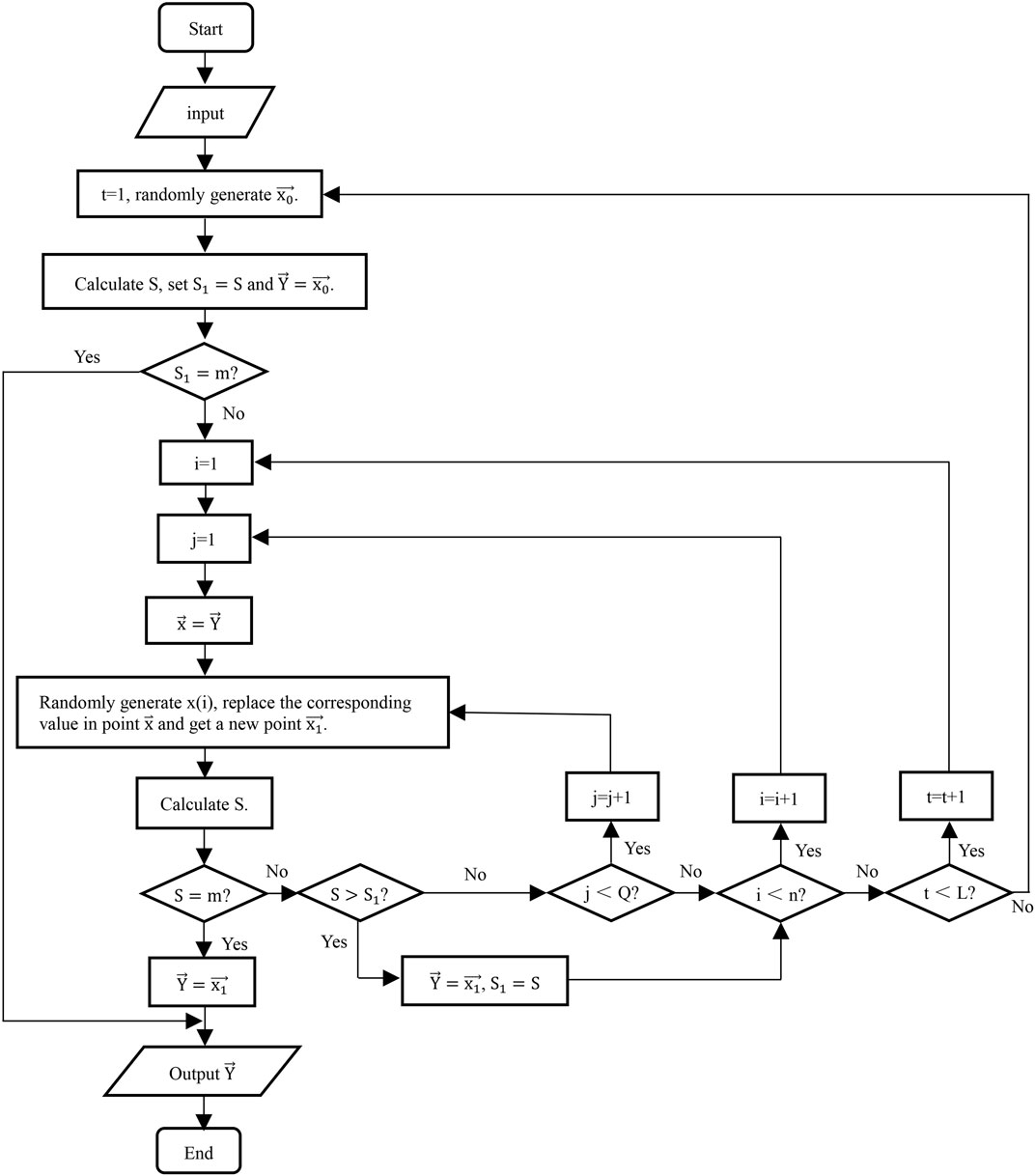
FIGURE 2. Flow chart of the initial feasible point search strategy.

2.3.2 Improvements to the CCE algorithm

The steps of the improved CCE algorithm for a single complex A are as follows:

Step 1:. $\mathrm{A}=\left\{\overrightarrow{{\mathrm{x}}_1},\overrightarrow{{\mathrm{x}}_2},\dots ,\overrightarrow{{\mathrm{x}}_{\mathrm{m}}}\right\}$ is a complex containing m sample points arranged in order of increasing objective function value, which is the input of the CCE algorithm.

Step 2:. Assign a probability to each point in A, ${\mathrm{p}}_{\mathrm{i}}=\frac{2\left(\mathrm{m}+1-\mathrm{i}\right)}{\mathrm{m}\left(\mathrm{m}+1\right)},\mathrm{i}=1,\dots ,\mathrm{m}$.

Step 3:. Randomly select q distinct points in A according to ${\mathrm{p}}_{\mathrm{i}}$ to construct a subcomplex. The locations of A that are used to construct the subcomplex are stored in L.

Step 4:. Replace the worst point in the subcomplex.

(a) Sort the points in the subcomplex B in order of the increasing objective function value. $\mathrm{B}=\left\{\overrightarrow{{\mathrm{u}}_1},\overrightarrow{{\mathrm{u}}_2},\dots ,\overrightarrow{{\mathrm{u}}_{\mathrm{q}-1}},\overrightarrow{{\mathrm{u}}_{\mathrm{q}}}\right\}$, $\overrightarrow{{\mathrm{u}}_{\mathrm{q}}}$ is the worst point in B. Compute the centroid of good points $\overrightarrow{\mathrm{g}}=\frac{{\displaystyle \sum }_{\mathrm{i}=1}^{\mathrm{q}-1}\overrightarrow{{\mathrm{u}}_{\mathrm{i}}}}{\mathrm{q}-1}$.

(b) Compute the reflection point $\overrightarrow{{\mathrm{x}}_{\mathrm{r}\mathrm{e}\mathrm{f}}}=2\overrightarrow{\mathrm{g}}-\overrightarrow{{\mathrm{u}}_{\mathrm{q}}}$, then compute the new point $\overrightarrow{\mathrm{r}}=\left(1-\theta \right)\overrightarrow{{\mathrm{x}}_{\mathrm{r}\mathrm{e}\mathrm{f}}}+\theta \overrightarrow{{\mathrm{u}}_1}$. This step moves the original reflection point to the best point $\overrightarrow{{\mathrm{u}}_1}$ by a certain distance and has been proved to enhance the efficiency of the original SCE-UA (Muttil and Jayawardena, 2008). The default value of θ is set to 0.2.

(c) If $\overrightarrow{\mathrm{r}}$ is a feasible point, compute its function value fr, and go to step (d); otherwise, generate a new feasible point $\overrightarrow{\mathrm{z}}$ by the improved mutation method (The detailed steps will be described later), set $\overrightarrow{\mathrm{r}}$ = $\overrightarrow{\mathrm{z}}$ and fr=fz.

(d) If fr < fq, replace $\overrightarrow{{\mathrm{u}}_{\mathrm{q}}}$ with $\overrightarrow{\mathrm{r}}$, and go to step (f); otherwise, compute the contraction point $\overrightarrow{{\mathrm{x}}_{\mathrm{c}\mathrm{o}\mathrm{n}}}=\frac{\overrightarrow{\mathrm{g}}+\overrightarrow{{\mathrm{u}}_{\mathrm{q}}}}{2}$, then compute the new point $\overrightarrow{\mathrm{c}}=\left(1-\theta \right)\overrightarrow{{\mathrm{x}}_{\mathrm{c}\mathrm{o}\mathrm{n}}}+\theta \overrightarrow{{\mathrm{u}}_1}$ and its function value fc. The default value of θ is also set to 0.2.

(e) If fc < fq and $\overrightarrow{\mathrm{c}}$ is feasible, replace $\overrightarrow{{\mathrm{u}}_{\mathrm{q}}}$ with $\overrightarrow{\mathrm{c}}$, and go to step (f); otherwise, use the improved mutation method to generate a mutation point $\overrightarrow{\mathrm{z}}$, and replace $\overrightarrow{{\mathrm{u}}_{\mathrm{q}}}$ with $\overrightarrow{\mathrm{z}}$.

(f) Repeat (a) through (e) α times, replacing the worst point in B each time.

Step 5:. Replace the corresponding points in A with the points in B according to the locations stored in L. Sort A in order of increasing function value.

Step 6:. Repeat Step 1∼Step 5 β times to complete the evolution of a complex.Figure 3 shows the flow chart of the improved CCE algorithm:The steps of the improved mutation method are as follows, it utilizes the location information of the known feasible points and guides the starting point to move to the centroid of A to search for the feasible mutation point.

FIGURE 3

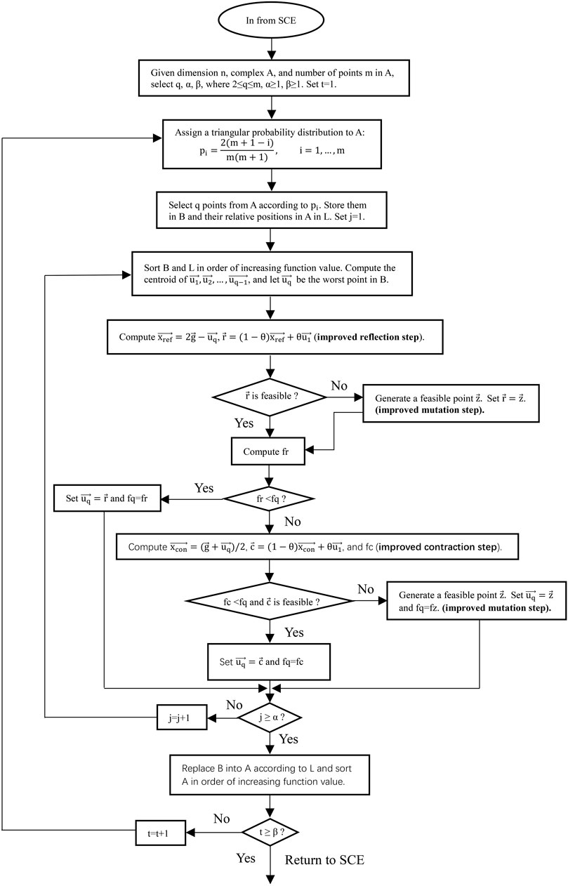
FIGURE 3. Flow chart of the improved CCE algorithm.

Step 1:. Randomly generate a starting point $\overrightarrow{{\mathrm{x}}_0}$ in the smallest hypercube H⊂ ${\mathrm{R}}^{\mathrm{n}}$ containing all points in A according to the uniform probability distribution in each dimension. If $\overrightarrow{{\mathrm{x}}_0}$ is feasible, set $\overrightarrow{\mathrm{z}}=\overrightarrow{{\mathrm{x}}_0}$, output $\overrightarrow{\mathrm{z}}$ and stop the mutation; else, go to step 2.

Step 2:. Compute the centroid of complex A, $\overrightarrow{{\mathrm{g}}_{\mathrm{A}}}=\frac{1}{\mathrm{m}}{\displaystyle \sum }_{\mathrm{i}=1}^{\mathrm{m}}\overrightarrow{{\mathrm{x}}_{\mathrm{i}}}$.

Step 3:. Set i=1, compute the new point $\overrightarrow{{\mathrm{x}}_1}=\overrightarrow{{\mathrm{x}}_0}+\lambda \left(\overrightarrow{{\mathrm{g}}_{\mathrm{A}}}-\overrightarrow{{\mathrm{x}}_0}\right)$, $\lambda =\frac{\mathrm{i}}{\mathrm{T}}$, T is the maximum number of adjustments based on the starting point $\overrightarrow{{\mathrm{x}}_0}$, and the default value is 10. If $\overrightarrow{{\mathrm{x}}_1}$ is feasible, set $\overrightarrow{\mathrm{z}}=\overrightarrow{{\mathrm{x}}_1}$, output $\overrightarrow{\mathrm{z}}$ and stop the mutation; otherwise, let i=2, … , T, recompute $\overrightarrow{{\mathrm{x}}_1}$ and determine whether it is in the feasible region. If no feasible mutation point is found after adjusting T times, go to step 4.

Step 4:. Return to step1, randomly generate a new $\overrightarrow{{\mathrm{x}}_0}$ in H. Repeat steps 1–4 until a feasible mutation point is found.The CSCE uses a new strategy to generate initial feasible points quickly and efficiently. Meanwhile, it adds feasibility review steps and uses the improved reflection step, the improved contraction step, and the improved mutation step to update points in the CCE algorithm. Due to the structural characteristics of the CSCE, there will be no infeasible points involved in the calculation of the objective function during the optimization process. Meanwhile, this method does not introduce new parameters, which is convenient for users to add constraints during optimization.

2.4 Termination criteria

To avoid the infinite loop of the algorithm, the termination criteria need to be set. In this paper, the termination criteria consist of the convergence criterion and the iteration criterion (Table 1). If any of them is met, the algorithm will stop.

TABLE 1

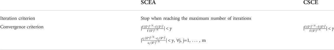
TABLE 1. Termination criteria for the algorithms.

Where ${\overrightarrow{\mathrm{x}}}^{*}$ in the above table is the best point in the current population. The CSCE will stop early if the objective function value does not change by convergence tolerance (γ) during the number of iterations N. However, the SCEA needs one more convergence criterion about constraints since the violation may still change in subsequent iterations, despite the convergence of the unpenalized objective function. This phenomenon was explained in detail by Lee and Kang (2016).

3 Experiment on test problems

This section shows a performance comparison between the CSCE and the SCEA on a suite of 14 test problems with inequality constraints. Table 2 shows the details of these test problems. 13 of these test problems were proposed in the IEEE Congress on Evolutionary Computation (Liang et al., 2006) and they have been widely used to test algorithms for constrained optimization problems. The last test problem (hereinafter referred to as T01, the formula is as follows) is described in (Deb, 2000). G06 and T01 were used to test the SCEA by Lee and Kang (2016).

$\begin{array}{c}\mathbf{T}\mathbf{01}:\mathbf{M}\mathbf{i}\mathbf{n}\mathbf{i}\mathbf{m}\mathbf{i}\mathbf{z}\mathbf{e}\mathbf{f}\left(\overrightarrow{\mathbf{x}}\right)={\left({\mathbf{x}}_{\mathbf{1}}^{\mathbf{2}}+{\mathbf{x}}_{\mathbf{2}}-\mathbf{11}\right)}^{\mathbf{2}}+{\left({\mathbf{x}}_{\mathbf{1}}+{\mathbf{x}}_{\mathbf{2}}^{\mathbf{2}}-\mathbf{7}\right)}^{\mathbf{2}}\\ \mathbf{s}\mathbf{u}\mathbf{b}\mathbf{j}\mathbf{e}\mathbf{c}\mathbf{t}\mathbf{t}\mathbf{o}\{\begin{array}{c}{\left({\mathbf{x}}_{\mathbf{1}}-\mathbf{0.05}\right)}^{\mathbf{2}}+{\left({\mathbf{x}}_{\mathbf{2}}-\mathbf{2.5}\right)}^{\mathbf{2}}-\mathbf{4.84}\le \mathbf{0}\\ {-\mathbf{x}}_{\mathbf{1}}^{\mathbf{2}}-{\left({\mathbf{x}}_{\mathbf{2}}-\mathbf{2.5}\right)}^{\mathbf{2}}+\mathbf{4.84}\le \mathbf{0}\\ \mathbf{0}\le {\mathbf{x}}_{\mathbf{1}}\le \mathbf{6},\mathbf{0}\le {\mathbf{x}}_{\mathbf{2}}\le \mathbf{6}\end{array}\end{array}(8)$

where the optimum solution is ${\overrightarrow{\mathrm{x}}}^{*}=\left(2.246826,2.3881865\right)$ with the corresponding function value ${\mathrm{f}(\overrightarrow{\mathrm{x}}}^{*})=13.59085$.

TABLE 2

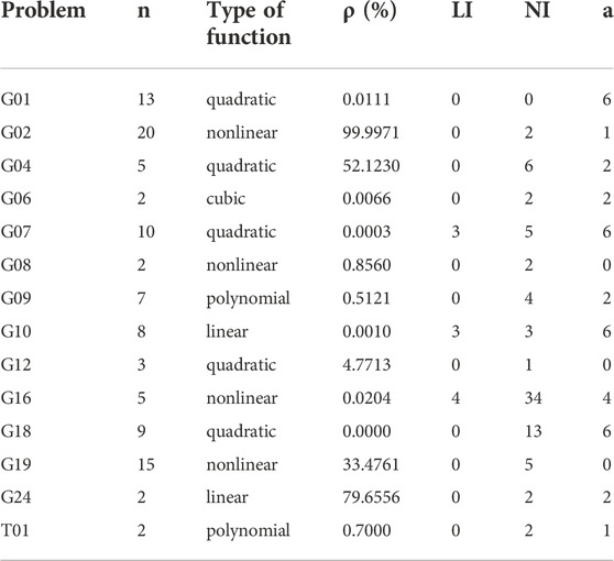
TABLE 2. Details of the test problems.

Where n is the number of decision variables; ρ is the ratio between the feasible region and the search space, which reflects the difficulty of searching feasible points; LI and NI represent the number of linear and nonlinear inequality constraints respectively; a is the number of active constraints at the optimum solution. Except for G12, the feasible region of each test problem is a convex set. The feasible region of G12 consists of 9³disjointed spheres. The following termination criteria were set: 1. The maximum number of iterations is 2000; 2. The iteration interval N=10 and the convergence toleranceγ=0.001%. For each test problem, the number of complexes p was set to the same value for the two algorithms, and the recommended values ​​were used for other parameters. Therefore, for each algorithm, the size of the initial population is (2n+1)p, and pαβ points are replaced in one iteration. Considering randomness, each algorithm was tested by running 30 times independently on each test problem. The minimum, median, maximum, mean, and standard deviation (STD) of the 30 results were recorded. The mean number of iterations (MI) was used to assess the algorithm’s convergence rate. Feasible rate (FR) refers to the proportion of feasible solutions in all results. Whether a trial is successful or not cannot be judged only by the objective function value corresponding to the solution. For example, the value of the function may be smaller than the theoretical optimum since the solution is outside the feasible region. Therefore, a trial will be deemed a success only if the solution is in the feasible region and its function value is close to the theoretical optimum ($\left|\mathrm{f}\left(\overrightarrow{\mathrm{x}}\right)-\mathrm{f}\left({\overrightarrow{\mathrm{x}}}^{*}\right)\right|\le 0.1$). Success rate (SR) refers to the proportion of the number of successful trials to the total number of trials. Table 3 shows the optimization results of the 14 test problems. The theoretical optimum corresponding to each problem is also listed in the first column.

TABLE 3

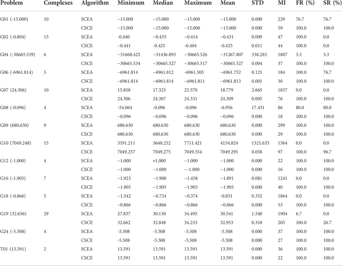
TABLE 3. Performance of the two algorithms on the test problems.

The first thing we notice is that due to the structural design of the CSCE, 100% of its solutions are feasible solutions, which is its greatest advantage. In contrast, the SCEA has a low proportion of feasible solutions for many problems, and there are even no feasible solutions in the results of G07, G10, G16, and G18, the feasible region of which are very narrow (ρ<0.02%). Although the SCEA often finds function values smaller than the theoretical optimal value in some problems such as G04, G07, G10, and G19, these solutions are outside the feasible region. This does not mean that there are no feasible points (r=0) in the population. Figure 4 shows an optimization process of G04. We can notice that the SCEA has a proportion of feasible individuals in each generation, but the final solution of G04 is often unfeasible. Furthermore, as the number of iterations increases, the value of the function fluctuates and fails to converge to the theoretical optimum value. When there are feasible individuals in the population (r>0), the modified objective function of SCEA is affected by the function value, the violation, and the status of the current population. In these problems, the infeasible points with small objective function values and violations are not necessarily eliminated but are likely to be retained because of small modified objective function values. In terms of the success rate, the CSCE has apparent advantages on all test problems except G02. 100% success rates are found in G01, G04, G06, G07, G08, G09, G12, G16, G18, G24, and T01. The SCEA can achieve high success rates in G01, G06, G08, G09, G12, G24, and T01, but the success rates in other problems are very low. G02 is a very complex function with a high dimension and its minimum value found by existing research is -0.804, the results of the two algorithms are near it but they both fail to find the theoretical minimum value. In terms of algorithm stability, the standard deviation of the optimization results of the CSCE is very small in each problem. In contrast, the stability of the SCEA is not good, especially in G04 and G10. The mean number of iterations of the CSCE is less than that of the SCEA, especially in G01, G04, G07, G10, G16, G18, and G19. Moreover, the CSCE achieves higher success rates in these problems, while the SCEA performs poorly. Both algorithms achieve a 100% success rate in G09, but the number of iterations required by the CSCE is far less than that of the SCEA. Overall, the CSCE can converge faster. A faster convergence speed is significant for the automatic calibration of hydrologic models because the structure of a hydrologic model is usually complex, and a large amount of data is involved in one computation. Therefore, more iterations mean more runs of the model, which is time-consuming.

FIGURE 4

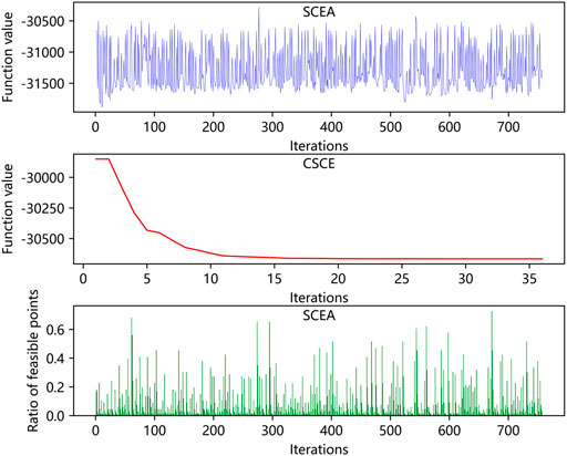
FIGURE 4. The optimization process of G04.

Lee and Kang (2016) only used T01 and G06 to test the SCEA, but it can be seen from our experiment that it is not comprehensive to test the SCEA on only two low-dimensional functions. The performance of the SCEA differs greatly for different problems. Overall, the CSCE is significantly better than the SCEA in terms of the success rate, stability, feasible rate, and convergence speed.

To test the CSCE algorithm’s ability to explore the whole feasible region, we initialized the algorithm with all its initial feasible population located in a very small region that is far away from the global optimum and observed whether the algorithm could expand the search scope and found the global optimal solution. The optimum solution of G04 is (78, 33, 29.995, 45, 36.776) where the function value is -30665.539, and the boundaries of variables are: $78\le x_1\le 102,33\le x_2\le 45,\mathrm{a}\mathrm{n}\mathrm{d}27\le x_i\le 45\left(\mathrm{i}=3,4,5\right)$. Using the strategy for generating initial feasible points, we generated 66 initial points (p=6) that satisfied all constraints of G04 in a very small hypercube far away from the global optimum solution ($101.8\le x_1\le 102,44.8\le x_2\le 45,44.8\le x_3\le 45,27\le x_4\le 27.2,27\le x_5\le 27.2$). Figure 5 shows the iteration curve of the CSCE in the case of different initial feasible populations. When using the random initial feasible population, the CSCE iterates 35 times and finds the solution (78.000, 33.000, 29.995, 45.000, 36.776) where the function value is -30665.520. When using the restricted initial feasible population in the small hypercube, the CSCE iterates 47 times and finds the solution (78.000, 33.000, 29.995, 45.000, 36.776) where the function value is -30665.531. The result indicates that the CSCE can explore the feasible region outside of the hypercube defined by the range of the initial feasible population during the optimization.

FIGURE 5

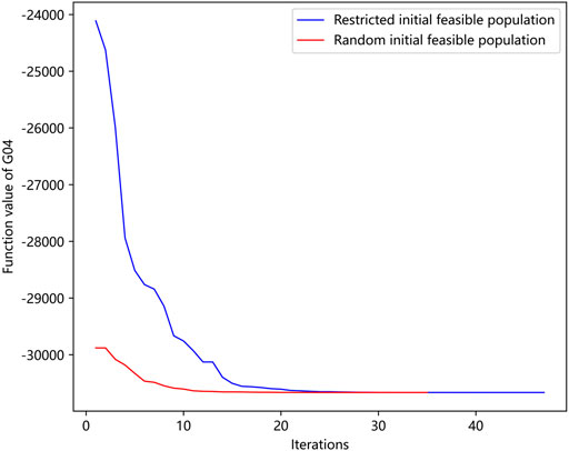
FIGURE 5. Iteration curve of the CSCE in the case of the different initial populations.

The success rates of the CSCE in G02 and G19 are not satisfactory. To compare the CSCE with more algorithms, some classic or modern optimization algorithms using the exterior penalty method were also used to solve these two problems. They were the differential evolution algorithm (DE) (Storn and Price, 1997), the genetic algorithm (Holland, 1992), the particle swarm optimization algorithm (PSO) (Shi et al., 1998), the sparrow search algorithm (SSA) (Xue and Shen, 2020), the seagull optimization algorithm (SOA) (Dhiman and Kumar, 2019), the whale optimization algorithm (WOA) (Mirjalili and Lewis, 2016), and the moth-flame optimization (MFOA) (Mirjalili, 2015). The following form of penalty function was used:

$\begin{array}{c}\mathrm{F}\left(\overrightarrow{\mathrm{x}}\right)=\mathrm{f}\left(\overrightarrow{\mathrm{x}}\right)+\mathrm{M}\sinh \left({\displaystyle \sum }_{\mathrm{j}=1}^{\mathrm{m}}\max \left({\mathrm{g}}_{\mathrm{j}}\left(\overrightarrow{\mathrm{x}}\right),0\right)\right)\end{array}(9)$

where M is the penalty parameter. To reduce the influence of the adjustment of M on the optimization results, the hyperbolic sine function was introduced to construct the penalty item, and the greater the violation value of all constraints, the faster the penalty item value increases. For each algorithm, the size of initial points was set to 574 for G02 and 868 for G19, corresponding to p=14 and p=28 in the CSCE. The number of iterations was set to 2000 without convergence judgment to show the complete optimization process of each algorithm (Figure 6). The penalty parameters and the parameters of each algorithm were determined by trial and error several times.

FIGURE 6

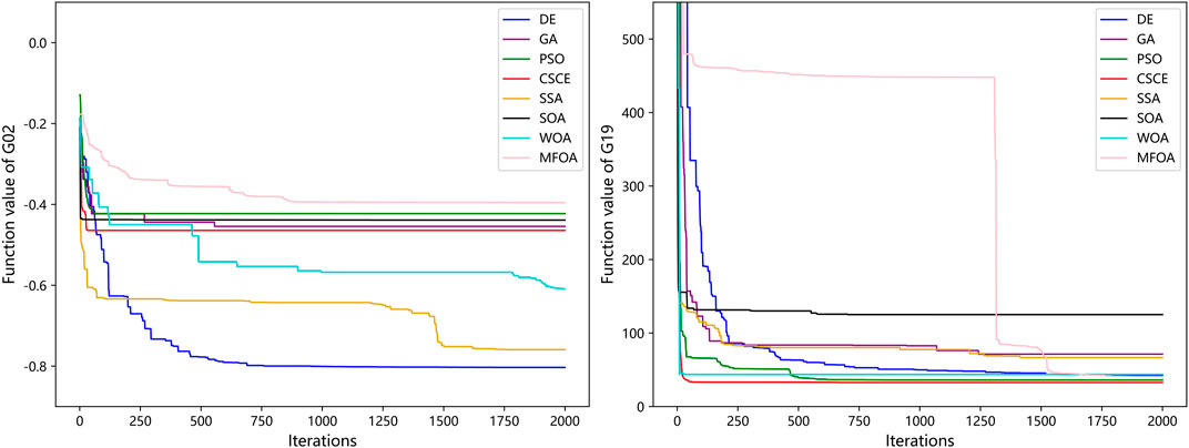
FIGURE 6. Iteration curves of different optimization algorithms for solving G02 and G19.

After 2000 iterations, the optimization results of the DE, the GA, the PSO, the CSCE, the SSA, the SOA, the WOA, and the MFOA are -0.803, -0.454, -0.423, -0.464, -0.759, -0.439, -0.609, -0.396 respectively for G02, and 42.639, 71.255, 36.075, 32.656, 66.606, 125.048, 43.668, 39.881 respectively for G19. These results are all feasible. In the optimization process of G02 and G19, the CSCE converges faster than most other algorithms. In contrast, some algorithms such as the DE, the GA, the SSA, and the MFOA have many apparent flat regions in their iteration curves where the function value changes very slowly. The CSCE outperforms all other algorithms in the optimization of G19, while its performance is not better than the DE, the SSA, and the WOA in G02.

4 Case study

The SCE-UA was originally invented to calibrate conceptual rainfall-runoff (CRR) models and has since been mainly used for the calibration of hydrologic and terrestrial models (Moradkhani and Sorooshian, 2008). The Xinanjiang (XAJ) model is a world-famous CRR model that has been widely used for runoff simulation and forecasting in humid and semi-humid areas. For detailed information about the XAJ model, please refer to the relevant paper (Zhao, 1992). The parameters of the XAJ model are listed in Table 4. Due to the correlation between the parameters, it is necessary to add some constraints during optimization. Among these constraints, the inequality WM-WUM-WLM>0 must be satisfied, otherwise the deep soil tension water capacity WDM will be negative, and the XAJ model program cannot run successfully. Few papers have mentioned this problem before. In previous studies, researchers usually increased the lower boundary of WM or changed to optimize WUM, WLM, and WDM (Cheng et al., 2006) to avoid this problem. However, compared with WDM, the research on WM is more comprehensive and the range of WM is easier to be estimated according to the climate and underlying conditions of the basin. In the National Flood Forecasting System of China (NFFS), the parameters WUM and WLM in the XAJ model are expressed as coefficients (${\mathrm{U}\mathrm{M}}_{\mathrm{x}}$ and ${\mathrm{L}\mathrm{M}}_{\mathrm{x}}$, the formula is as follows) rather than their absolute values. This method can avoid WDM<0 during optimization, but it enhances the correlation between parameters in the optimization process and makes the parameters difficult to understand, especially when training hydrological forecasters.

$\begin{array}{c}\mathbf{W}\mathbf{U}\mathbf{M}={\mathbf{U}\mathbf{M}}_{\mathbf{x}}·\mathbf{W}\mathbf{M}\\ \mathbf{W}\mathbf{L}\mathbf{M}={\mathbf{L}\mathbf{M}}_{\mathbf{x}}·\left(\mathbf{W}\mathbf{M}-\mathbf{W}\mathbf{U}\mathbf{M}\right)\\ \mathbf{W}\mathbf{D}\mathbf{M}=\mathbf{W}\mathbf{M}-\mathbf{W}\mathbf{U}\mathbf{M}-\mathbf{W}\mathbf{L}\mathbf{M}\\ {\mathbf{U}\mathbf{M}}_{\mathbf{x}},{\mathbf{L}\mathbf{M}}_{\mathbf{x}}\mathbf{\in }\mathbf{\left(}\mathbf{0}\mathbf{,}\mathbf{1}\mathbf{\right)}\end{array}(10)$

TABLE 4

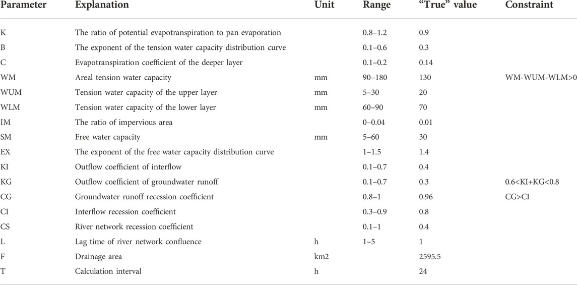
TABLE 4. Parameters of the XAJ model using synthetic data.

The CSCE can fundamentally avoid this trouble since the infeasible parameter sets will be directly eliminated in the optimization process and will not be input into the XAJ model. To verify its effectiveness and convenience in the automatic calibration of hydrologic models, the CSCE was applied to the calibration of the XAJ model. The synthetic data were used to test whether the CSCE could find the theoretical optimal parameters of the XAJ model under the constraints, and the observed data was used to test its application effect.

4.1 Study area and data

The Hexi Basin is located in northwestern Hunan Province, China. It is a typical fan-shaped basin with a drainage area of 2595.5 km². The Hexi hydrometric station is located at the outlet of the basin, which plays an important role in the flood defense of the basin and has been a key station in flood forecasting research in recent years. The observed precipitation, pan evaporation, and discharge data of the Hexi basin from 1/1/2014 to 31/10/2020 were collected, including long series of daily data, and hourly data of 20 rainfall-runoff events. The areal precipitation of the basin was calculated using the Thiessen polygon method based on the five rain gauging stations (Duoxi station, Aizhai station, Sangongqiao station, Xinglongchang station, and Hexi station). Figure 7 shows the station distribution of the Hexi Basin.

FIGURE 7

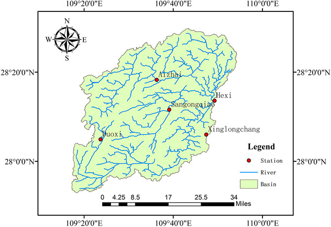
FIGURE 7. Study area and station distribution.

4.2 Optimization based on synthetic data

This section shows the performance of the CSCE in the calibration of the XAJ model using synthetic discharge data. The long series of daily areal precipitation and pan evaporation data for the basin from 1/1/2014 to 31/10/2020 were input into the XAJ model, and a set of parameters were specified as “true” (i.e., known) parameters ​​to generate synthetic discharge data. This method can artificially eliminate the model structure error and the observational error (Li et al., 2013) so that the theoretical optimal value of each parameter is known, and then help us to know whether the CSCE can retrieve the “true” values of the parameters of the XAJ model under the given range and constraints. Table 4 shows the ranges, “true” values, ​​and constraints of the XAJ model parameters.

The values of F and T were already known, so there were 15 parameters to be optimized. The lag time of river network confluence is required to be an integer, but the SCE-UA algorithm does not consider integer programming, so L was allowed to be input into the objective function in decimal form, but it needed to be rounded to an integer before being input into the XAJ model. KI+KG reflects the runoff recession duration of the basin, and its value is approximately 0.7 for the medium basin with a duration of 3 days (Zhang et al., 2015). The shorter the runoff recession duration is, the larger the value of KI+KG. Therefore, 0.6<KI+KG<0.8 was set according to the conditions of the Hexi Basin. CG>CI was set since the runoff recession of interflow is often faster than that of underground runoff. The mean square error (MSE) of the simulated discharge process and the ideal discharge process was taken as the objective function:

$\begin{array}{c}{\mathbf{F}}_{\mathbf{o}\mathbf{b}\mathbf{j}}=\mathbf{M}\mathbf{S}\mathbf{E}=\frac{\mathbf{1}}{\mathbf{k}}{\displaystyle \sum }_{\mathbf{i}=\mathbf{1}}^{\mathbf{k}}{\left[\mathbf{y}\left(\mathbf{i}\right)-{\mathbf{y}}_{\mathbf{0}}\left(\mathbf{i}\right)\right]}^{\mathbf{2}}\end{array}(11)$

where $\mathrm{y}\left(\mathrm{i}\right)$ is the ith simulation value; ${\mathrm{y}}_0\left(\mathrm{i}\right)$ is the ith observed value; k is the length of the sequence; and ${\mathrm{F}}_{\mathrm{o}\mathrm{b}\mathrm{j}}$ is the objective function. The number of complexes p was set to 8. The following termination criteria were set: 1. The maximum number of iterations is 1000; 2. the iteration interval N=10 and the convergence toleranceγ=0.001%. The CSCE was run 10 times independently and the results are shown in Table5. The result of each parameter is rounded to 2 decimal places.

TABLE 5

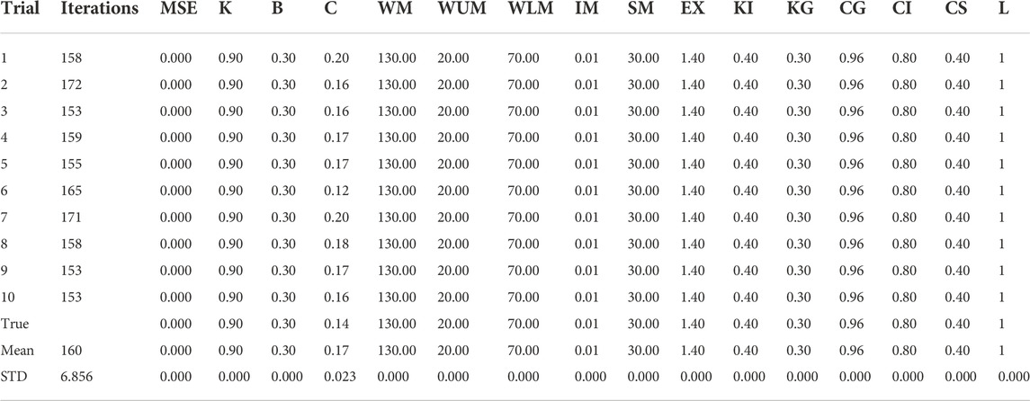
TABLE 5. Parameter calibration results using synthetic data.

This is a constrained optimization problem with 15 decision variables. We can notice from the table that except for parameter C, the CSCE can find out the theoretical optimum of each parameter very accurately in each run. C is a very insensitive parameter in the XAJ model and has little impact on the runoff process, so its optimization results are not equal to 0.14 but always around it. The standard deviation corresponding to each parameter is small and close to zero, which means that for different initial populations, the CSCE can always converge to the theoretically optimal parameter set of the XAJ model under the constraints.

4.3 Optimization based on observed data

The hourly data of 20 rainfall-runoff events from 2014 to 2020 were used to construct the XAJ model, of which 16 floods were used for calibration and 4 floods were used for validation. As demonstrated by Lu and Li (2015), reducing the number of dimensions and the range of parameters can effectively improve the convergence of the optimization and the possibility of obtaining a globally optimal solution. Therefore, some insensitive parameters were fixed: B=0.4, C=0.14, and EX=1.4. The following constraints were set: WM-WUM-WLM>0, 0.6<KI+KG<0.8, and CI<CG. The CSCE was used to optimize the remaining 12 parameters, p=7, and the remaining parameters of the SCE-UA were set to the recommended values.

Flood peak, flood volume, and flood process are the key points in flood forecasting. It is difficult to comprehensively evaluate the simulation effect using a single objective function. Therefore, the objective function was set as a combination of the peak relative error (PRE), the flood volume error (FVE), and the Nash-Sutcliffe efficiency coefficient (Moriasi et al., 2015). The mean absolute error (MAE) and the mean relative error (MRE) were also used to quantify the simulation effect. The following termination criteria were set: 1. The maximum number of iterations is 1000; 2. the iteration interval N=10 and the convergence toleranceγ=0.001%.

$\begin{array}{c}\mathbf{P}\mathbf{R}\mathbf{E}=\left(\mathbf{Y}-{\mathbf{Y}}_{\mathbf{0}}\right)/{\mathbf{Y}}_{\mathbf{0}}\end{array}(12)$

$\begin{array}{c}\mathbf{F}\mathbf{V}\mathbf{E}={\displaystyle \sum }_{\mathbf{i}=\mathbf{1}}^{\mathbf{k}}\left[\mathbf{y}\left(\mathbf{i}\right)-{\mathbf{y}}_{\mathbf{0}}\left(\mathbf{i}\right)\right]/{\displaystyle \sum }_{\mathbf{i}=\mathbf{1}}^{\mathbf{k}}{\mathbf{y}}_{\mathbf{0}}\left(\mathbf{i}\right)\end{array}(13)$

$\begin{array}{c}\mathbf{N}\mathbf{S}\mathbf{E}=\mathbf{1}-\frac{{{\sum }_{\mathbf{i}=\mathbf{1}}^{\mathbf{k}}\left[\mathbf{y}\left(\mathbf{i}\right)-{\mathbf{y}}_{\mathbf{0}}\left(\mathbf{i}\right)\right]}^{\mathbf{2}}}{{{\sum }_{\mathbf{i}=\mathbf{1}}^{\mathbf{k}}\left[{\mathbf{y}}_{\mathbf{0}}\left(\mathbf{i}\right)-\overline{{\mathbf{y}}_{\mathbf{0}}}\right]}^{\mathbf{2}}}\end{array}(14)$

$\begin{array}{c}{\mathbf{F}}_{\mathbf{o}\mathbf{b}\mathbf{j}}={\mathbf{F}}_{\mathbf{1}}+{\mathbf{F}}_{\mathbf{2}}-{\mathbf{F}}_{\mathbf{3}}=\frac{\mathbf{1}}{\mathbf{F}}{\sum }_{\mathbf{i}=\mathbf{1}}^{\mathbf{F}}\left|{\mathbf{P}\mathbf{R}\mathbf{E}}_{\mathbf{i}}\right|+\frac{\mathbf{1}}{\mathbf{F}}{\sum }_{\mathbf{i}=\mathbf{1}}^{\mathbf{F}}\left|{\mathbf{F}\mathbf{V}\mathbf{E}}_{\mathbf{i}}\right|-\frac{\mathbf{1}}{\mathbf{F}}{\sum }_{\mathbf{i}=\mathbf{1}}^{\mathbf{F}}{\mathbf{N}\mathbf{S}\mathbf{E}}_{\mathbf{i}}\end{array}(15)$

$\begin{array}{c}\mathbf{M}\mathbf{A}\mathbf{E}=\frac{\mathbf{1}}{\mathbf{k}}{\displaystyle \sum }_{\mathbf{i}=\mathbf{1}}^{\mathbf{k}}\left|\mathbf{y}\left(\mathbf{i}\right)-{\mathbf{y}}_{\mathbf{0}}\left(\mathbf{i}\right)\right|\end{array}(16)$

$\begin{array}{c}\mathbf{M}\mathbf{R}\mathbf{E}=\frac{\mathbf{1}}{\mathbf{k}}{\displaystyle \sum }_{\mathbf{i}=\mathbf{1}}^{\mathbf{k}}\left|\mathbf{y}\left(\mathbf{i}\right)-{\mathbf{y}}_{\mathbf{0}}\left(\mathbf{i}\right)\right|/{\mathbf{y}}_{\mathbf{0}}\left(\mathbf{i}\right)\end{array}(17)$

where $\mathrm{Y}$ represents the simulated peak discharge; ${\mathrm{Y}}_0$ represents the observed peak discharge; $\mathrm{y}\left(\mathrm{i}\right)$ is the ith simulation value; ${\mathrm{y}}_0\left(\mathrm{i}\right)$ is the ith observed value; k is the length of the sequence; $\overline{{\mathrm{y}}_0}$ is the mean of the observed values; F is the number of floods for calibration. Table 6 shows the parameter results optimized by the CSCE.

TABLE 6

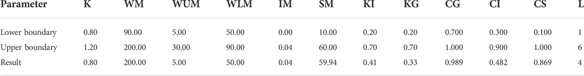
TABLE 6. Parameter calibration results using observed data.

The SCEA was also used for comparison. The termination criteria and the number of complexes are the same as those of the CSCE. WUM, WLM, and WDM were optimized instead of WM, WUM, and WLM to avoid WDM<0. The range of the WDM was set to 25–60 mm. Table 7 shows the comparison of the two algorithms.

TABLE 7

TABLE 7. Results of the two algorithms in the calibration of the XAJ model using observed data.

We can notice that the CSCE achieves a smaller objective function value with fewer iterations and each item of the objective function (${\mathrm{F}}_1,{\mathrm{F}}_2,\mathrm{a}\mathrm{n}\mathrm{d}-{\mathrm{F}}_3$) has a better value than the result of the SCEA. This means that the XAJ model optimized by the CSCE has a better simulation performance in terms of the flood peak, flood volume, and flood process in the calibration period. During the optimization process, the SCEA needs to run the XAJ model 22006 times while the CSCE only needs 16627 times. Table 8 shows the error statistics of the simulation results. MAV is the mean absolute value.

TABLE 8

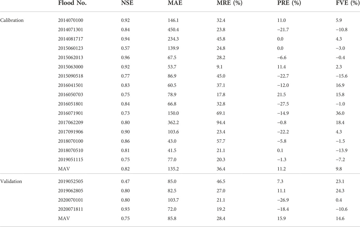
TABLE 8. Simulation error statistics of the XAJ model optimized by the CSCE.

The XAJ model optimized by the CSCE has a good simulation effect in the calibration period and the validation period. Each simulated flood has a high NSE or small peak error. The MAV of the NSE is between 0.7 and 0.9 in both periods and the simulation precision achieves the B standard according to the standard for hydrological information and hydrological forecasting in China. In terms of the process simulation effect, the NSE is greater than 0.9 for six floods, between 0.7 and 0.9 for 12 floods, between 0.5 and 0.7 for one flood, and less than 0.5 for only one flood. In terms of the peak simulation effect, the absolute value of the PRE is less than 10% for eight floods, between 10% and 20% for six floods, and between 20% and 30% for six floods. In terms of the flood volume simulation effect, the absolute value of the FVE is less than 10% for 10 floods, between 10% and 20% for seven floods, and greater than 20% for three floods. Overall, the XAJ model optimized by the CSCE can effectively simulate the hourly rainfall-runoff events in the basin.

5 Conclusion

In this paper, the CSCE algorithm is proposed to solve inequality-constrained optimization problems and is compared with the SCEA and some other algorithms. According to its performance on the test problems and the XAJ model, we draw the following conclusions: (1) The CSCE is more advantageous than the SCEA in terms of the success rate, stability, feasible rate, and convergence speed. It performs well on most test problems, while the performance of the SCEA differs greatly in different problems. (2) The CSCE only searches for the optimal solution in the feasible region, this feature can guarantee the feasibility of the solution and avoid the problem of WDM<0 in the optimization process of the XAJ model. (3) When using synthetic data, the CSCE can accurately find the theoretical optimal parameters of the XAJ model under the given constraints. When using observed data, the XAJ model optimized by the CSCE can effectively simulate the hourly rainfall-runoff events in the Hexi Basin.

The SCE-UA is a classical algorithm in the field of hydrology. On the one hand, we propose the CSCE for solving inequality-constrained optimization problems and prove its effectiveness, on the other hand, we use more problems to test the SCEA and find its shortcomings, which is also a complement to the existing studies. However, the CSCE still deserves further exploration. When the feasible region is narrow, the search for feasible points takes extra time, which is obvious in the optimization of G07 and G18. The smaller the feasible region, the greater the time cost for the CSCE to search for feasible points. As demonstrated in the experiment on G04, when the feasible domain is a convex set, the CSCE can expand the search scope and find the optimal solution despite the initial feasible points being compressed in a small range. However, when the feasible domain is discrete and the initial feasible points are restricted in a small range at the same time, the CSCE may face difficulties in jumping between sub-feasible domains, in which case the diversity of initial feasible points becomes more important. In addition, this paper only shows its application in the calibration of the hydrologic model. As a new optimization tool, its application effect on reservoir operation, optimal allocation of water resources, and other domains are also worthy of further study.

Data availability statement

The original contributions presented in the study are included in the article/supplementary material further inquiries can be directed to the corresponding author.

Author contributions

CJ contributed to the conceptualization, methodology, software, formal analysis, and manuscript writing of the study; SZ contributed to the review, supervision, project administration, and funding acquisition of the study; YX contributed to the validation, review, editing, and revision of the paper.

Funding

This research was supported by the Science and Technology Planning Project of Guangdong Province (No: 2020B1212030005); the Key Research and Development Program of Hunan Province (No: 2020SK2130).

Acknowledgments

We thank Yi Xiao for his suggestions on the format modification and submission of this article.

Conflict of interest

The authors declare that the research was conducted in the absence of any commercial or financial relationships that could be construed as a potential conflict of interest.

Publisher’s note

All claims expressed in this article are solely those of the authors and do not necessarily represent those of their affiliated organizations, or those of the publisher, the editors and the reviewers. Any product that may be evaluated in this article, or claim that may be made by its manufacturer, is not guaranteed or endorsed by the publisher.

References

Ajami, N. K., Gupta, H., Wagener, T., and Sorooshian, S. (2004). Calibration of a semi-distributed hydrologic model for streamflow estimation along a river system. J. Hydrology 298 (1-4), 112–135. doi:10.1016/j.jhydrol.2004.03.033

CrossRef Full Text | Google Scholar

Arsenault, R., Poulin, A., Cote, P., and Brissette, F. (2014). Comparison of stochastic optimization algorithms in hydrological model calibration. J. Hydrol. Eng. 19 (7), 1374–1384. doi:10.1061/(asce)he.1943-5584.0000938

CrossRef Full Text | Google Scholar

Askarzadeh, A. (2016). A novel metaheuristic method for solving constrained engineering optimization problems: Crow search algorithm. Comput. Struct. 169, 1–12. doi:10.1016/j.compstruc.2016.03.001

CrossRef Full Text | Google Scholar

Ayad, A., Khalifa, A., Fawy, M. E., and Moawad, A. (2021). An integrated approach for non-revenue water reduction in water distribution networks based on field activities, optimisation, and GIS applications. Ain Shams Eng. J. 12 (4), 3509–3520. doi:10.1016/j.asej.2021.04.007

CrossRef Full Text | Google Scholar

Chang, L.-C., Chang, F.-J., Wang, K.-W., and Dai, S.-Y. (2010). Constrained genetic algorithms for optimizing multi-use reservoir operation. J. Hydrology 390 (1-2), 66–74. doi:10.1016/j.jhydrol.2010.06.031

CrossRef Full Text | Google Scholar

Cheng, C. T., Zhao, M. Y., Chau, K. W., and Wu, X. Y. (2006). Using genetic algorithm and TOPSIS for Xinanjiang model calibration with a single procedure. J. Hydrology 316 (1-4), 129–140. doi:10.1016/j.jhydrol.2005.04.022

CrossRef Full Text | Google Scholar

Cooper, V. A., Nguyen, V. T. V., and Nicell, J. A. (1997). Evaluation of global optimization methods for conceptual rainfall-runoff model calibration. Water Sci. Technol. 36 (5), 53–60. doi:10.2166/wst.1997.0163

CrossRef Full Text | Google Scholar

Deb, K. (2000). An efficient constraint handling method for genetic algorithms. Comput. Methods Appl. Mech. Eng. 186 (2-4), 311–338. doi:10.1016/s0045-7825(99)00389-8

CrossRef Full Text | Google Scholar

Dhiman, G., and Kumar, V. (2019). Seagull optimization algorithm: Theory and its applications for large-scale industrial engineering problems. Knowledge-Based Syst. 165, 169–196. doi:10.1016/j.knosys.2018.11.024

CrossRef Full Text | Google Scholar

Duan, Q. Y., Gupta, V. K., and Sorooshian, S. (1993). Shuffled complex evolution approach for effective and efficient global minimization. J. Optim. Theory Appl. 76 (3), 501–521. doi:10.1007/bf00939380

CrossRef Full Text | Google Scholar

Duan, Q. Y., Sorooshian, S., and Gupta, V. K. (1994). Optimal use of the sce-ua global optimization method for calibrating watershed models. J. Hydrology 158 (3-4), 265–284. doi:10.1016/0022-1694(94)90057-4

CrossRef Full Text | Google Scholar

Eusuff, M. M., and Lansey, K. E. (2004). Optimal operation of artificial groundwater recharge systems considering water quality transformations. Water Resour. Manag. 18 (4), 379–405. doi:10.1023/B:WARM.0000048486.46046.ee

CrossRef Full Text | Google Scholar

Farmani, R., and Wright, J. A. (2003). Self-adaptive fitness formulation for constrained optimization. IEEE Trans. Evol. Comput. 7 (5), 445–455. doi:10.1109/tevc.2003.817236

CrossRef Full Text | Google Scholar

Guo, Q., Ba, J., and Luo, C. (2021). Prestack seismic inversion with data-driven MRF-based regularization. IEEE Trans. Geosci. Remote Sens. 59 (8), 7122–7136. doi:10.1109/tgrs.2020.3019715

CrossRef Full Text | Google Scholar

Gupta, K., Deep, K., and Bansal, J. C. (2017). Spider monkey optimization algorithm for constrained optimization problems. Soft Comput. 21 (23), 6933–6962. doi:10.1007/s00500-016-2419-0

CrossRef Full Text | Google Scholar

Holland, J. H. (1992). Adaptation in natural and artificial systems: An introductory analysis with applications to biology, control, and artificial intelligence [M]. 2nd ed. Cambridge, MA, USA. MIT Press.

Google Scholar

Jayawardena, A. W., Muttil, N., and Lee, J. H. W. (2006). Comparative analysis of data-driven and GIS-based conceptual rainfall-runoff model. J. Hydrol. Eng. 11 (1), 1–11. doi:10.1061/(asce)1084-0699(2006)11:1(1)11:1(1

CrossRef Full Text | Google Scholar

Kan, G. Y., Liang, K., Li, J. R., Ding, L. Q., He, X. Y., and Hu, Y. B., (2016). Accelerating the SCE-UA global optimization method based on multi-core CPU and many-core GPU. Adv. Meteorology 2016, 1–10. doi:10.1155/2016/8483728

CrossRef Full Text | Google Scholar

Kang, T., and Lee, S. (2014). Modification of the SCE-UA to include constraints by embedding an adaptive penalty function and application: Application approach. Water Resour. manage. 28 (8), 2145–2159. doi:10.1007/s11269-014-0602-6

CrossRef Full Text | Google Scholar

Ketabchi, H., and Ataie-Ashtiani, B. (2015). Evolutionary algorithms for the optimal management of coastal groundwater: A comparative study toward future challenges. J. Hydrology 520, 193–213. doi:10.1016/j.jhydrol.2014.11.043

CrossRef Full Text | Google Scholar

Le Ngo, L., Madsen, H., and Rosbjerg, D. (2007). Simulation and optimisation modelling approach for operation of the Hoa Binh reservoir, Vietnam. J. Hydrology 336 (3-4), 269–281. doi:10.1016/j.jhydrol.2007.01.003

CrossRef Full Text | Google Scholar

Lee, S., and Kang, T. (2016). Analysis of constrained optimization problems by the SCE-UA with an adaptive penalty function. J. Comput. Civ. Eng. 30 (3). doi:10.1061/(asce)cp.1943-5487.0000493

CrossRef Full Text | Google Scholar

Li, Z., Xin, P., and Tang, J. (2013). Study of the Xinanjiang model parameter calibration. J. Hydrol. Eng. 18 (11), 1513–1521. doi:10.1061/(asce)he.1943-5584.0000527

CrossRef Full Text | Google Scholar

Liang, J. J., Runarsson, T. P., Mezura-Montes, E., Clerc, M., and Deb, K. (2006). Problem definitions and evaluation criteria for the CEC 2006 special session on constrained real-parameter optimization. J. Appl. Mech. 41 (8), 8–31.

Google Scholar

Liu, X. E., Zhang, S. J., and Zhang, X. L. (2001). The search for feasible initial point in constrained optimization design. J. Xi'an Univ. Archit. Technol. 2001 (04), 340–343. (in Chinese). doi:10.3969/j.issn.1006-7930.2001.04.009

CrossRef Full Text | Google Scholar

Lu, M., and Li, X. (2015). Strategy to automatically calibrate parameters of a hydrological model: A multi-step optimization scheme and its application to the Xinanjiang model. Hydrological Res. Lett. 9 (4), 69–74. doi:10.3178/hrl.9.69

CrossRef Full Text | Google Scholar

Mirjalili, S., and Lewis, A. (2016). The whale optimization algorithm. Adv. Eng. Softw. 95, 51–67. doi:10.1016/j.advengsoft.2016.01.008

CrossRef Full Text | Google Scholar

Mirjalili, S. (2015). Moth-flame optimization algorithm: A novel nature-inspired heuristic paradigm. Knowledge-Based Syst. 89, 228–249. doi:10.1016/j.knosys.2015.07.006

CrossRef Full Text | Google Scholar

Moradkhani, H., and Sorooshian, S. (2008). “General review of rainfall-runoff modeling: Model calibration, data assimilation, and uncertainty analysis”. in: Summer Sch. Hydrologic Model. Water Cycle. Springer, Berlin, Germany, 1-24. doi:10.1007/978-3-540-77843-1_1

CrossRef Full Text | Google Scholar

Moriasi, D. N., Gitau, M. W., Pai, N., and Daggupati, P. (2015). Hydrologic and water quality models: Performance measures and evaluation criteria. Trans. Asabe 58 (6), 1763–1785.

Google Scholar

Muttil, N., and Jayawardena, A. W. (2008). Shuffled complex evolution model calibrating algorithm: Enhancing its robustness and efficiency. Hydrol. Process. 22 (23), 4628–4638. doi:10.1002/hyp.7082

CrossRef Full Text | Google Scholar

Naeini, M. R., Analui, B., Gupta, H. V., Duan, Q., and Sorooshian, S. (2019). Three decades of the shuffled complex evolution (SCE-UA) optimization algorithm: Review and applications. Sci. Iran. 26 (4), 2015–2031. doi:10.24200/sci.2019.21500

CrossRef Full Text | Google Scholar

Nelder, J. A., and Mead, R. (1965). A simplex-method for function minimization. Comput. J. 7 (4), 308–313. doi:10.1093/comjnl/7.4.308

CrossRef Full Text | Google Scholar

Shi, Y. H., and Eberhart, R. (1998). A modified particle swarm optimizer. IEEE Int. Conf. Evol. Comput., 69–73.

Google Scholar

Storn, R., and Price, K. (1997). Differential evolution - a simple and efficient heuristic for global optimization over continuous spaces. J. Glob. Optim. 11 (4), 341–359. doi:10.1023/a:1008202821328

CrossRef Full Text | Google Scholar

Tessema, B., and Yen, G. G. (2009). An adaptive penalty formulation for constrained evolutionary optimization. IEEE Trans. Syst. Man. Cybern. A 39 (3), 565–578. doi:10.1109/tsmca.2009.2013333

CrossRef Full Text | Google Scholar

Vrugt, J. A., Gupta, H. V., Bastidas, L. A., Bouten, W., and Sorooshian, S. (2003). Effective and efficient algorithm for multiobjective optimization of hydrologic models. Water Resour. Res. 39 (8). doi:10.1029/2002wr001746

CrossRef Full Text | Google Scholar

Vrugt, J. A., Gupta, H. V., Bouten, W., and Sorooshian, S. (2003). A Shuffled Complex Evolution Metropolis algorithm for optimization and uncertainty assessment of hydrologic model parameters. Water Resour. Res. 39 (8). doi:10.1029/2002wr001642

CrossRef Full Text | Google Scholar

Xue, J. K., and Shen, B. (2020). A novel swarm intelligence optimization approach: Sparrow search algorithm. Syst. Sci. Control Eng. 8 (1), 22–34. doi:10.1080/21642583.2019.1708830

CrossRef Full Text | Google Scholar

Yapo, P. O., Gupta, H. V., and Sorooshian, S. (1998). Multi-objective global optimization for hydrologic models. J. Hydrology 204 (1-4), 83–97. doi:10.1016/s0022-1694(97)00107-8

CrossRef Full Text | Google Scholar

Zhang, C., Wang, R.-b., and Meng, Q.-x. (2015). Calibration of conceptual rainfall-runoff models using global optimization. Adv. Meteorology 2015, 1–12. doi:10.1155/2015/545376

CrossRef Full Text | Google Scholar

Zhao, R. J. (1992). The xinanjiang model applied in China. J. Hydrology 135 (1-4), 371–381. doi:10.1016/0022-1694(92)90096-e

CrossRef Full Text | Google Scholar