Quantitative prediction of multistage fractures of ultra-deep tight sandstone based on the theory of minimum energy dissipation

Due to strong reservoir heterogeneity and low-resolution limit of geophysical data, it is difficult to predict fractures in ultra-deep reservoirs by conventional methods. In this research, we established a novel geomechanical model for prediction of fracture distribution in brittle reservoirs, especially for ultra-deep tight sandstone reservoirs. Methodologically, we intended to introduce the minimum energy dissipation principle considering time variable, combined with the generalized Hooke’s law containing damage variable, and obtained the energy dissipation rate expression corresponding to the energy dissipation process of brittle rocks. Combined with the three-shear energy yield criterion, the Lagrangian multiplier was introduced to deduce and construct the constitutive model and the failure criterion of rocks under the framework of the theory of minimum energy dissipation. Based on the law of conservation of energy, the stress-energy coupling characterization model of fracture density parameter was derived. Finally, all the improved geomechanical equations were incorporated into a finite element software to quantitatively simulate the distributions of tectonic stress filed and fractures based on paleo-structure restoration of Keshen anticline during the middle and late Himalayan periods. Its predictions agreed well with measured fracture density from reservoir cores and image logs.

1 Introduction

As an important unconventional resource and clean-burning fuel, tight sandstone gas has been widely distributed in many countries in the world, such as the U.S., Canada, Australia, Mexico, Russia, and China (Conti et al., 2016; Lu et al., 2016; Song et al., 2017; Zhou et al., 2021). In general, tight sandstone reservoirs distinctively differ from conventional reservoirs due to their unique geological features including great burial depth, strong diagenesis, strong heterogeneity, abnormal overpressure, low porosity and developed fractures (Shrivastava and Lawatia, 2011; Walderhaug et al., 2012; Xue et al., 2014; Ding et al., 2015; Wang et al., 2016). In these tight low-permeability sandstones, the majority of reservoir spaces and seepage channels for hydrocarbon are primarily provided by widely distributed natural fractures, especially structural fractures, which can significantly and effectively improve the permeability of a reservoir and enhance hydrocarbon delivery to wellbores (DeJarnett et al., 2001; Laubach, 2003; Cumella and Scheevel, 2008; Taylor et al., 2010; Solano et al., 2011; Shanley and Cluff, 2015; Ju et al., 2017). Therefore, understanding and interpreting where and when structural fractures develop within a geological structure, along with their orientation, intensity and porosity are important in both exploration and production of tight sandstone reservoirs. However, how to predict fractures effectively is still a worldwide challenge. Three-dimensional (3-D) characterization and modeling of subsurface structural fractures pose a greater challenge in deep tight sandstone gas reservoirs with complex tectonism and diagenesis (McLennan et al., 2009; Olson et al., 2009; Deng et al., 2013; Zeng et al., 2017; Ay et al., 2019).

Models based on geometry and/or kinematics such as analyses of fault-related folds and fold curvature (Lisle, 1994; Hennings et al., 2000; Sanz et al., 2008; Ju et al., 2014; Feng et al., 2020), seismic techniques or logging methods are commonly used in fracture reservoir exploration and production and fracture prediction or modeling. In recent years and advancement of artificial intelligence technology based on a large amount of drilling measurement data, some researchers have employed the use of neural networks or deep-learning methods to predict the space of subsurface fractures. These approaches which aims to acquire the attributes of inter-well fracture networks, rely on measured data and relate the deformation to corresponding structural position (Smart et al., 2012). They are commonly tied to ideal geometric models or simplified assumptions that may not completely reflect the multi-phase deformation behaviors and mechanical properties of underground rocks (Laubach, 2003; Olson et al., 2009; Smart et al., 2012).

Generally, tectonic stress field is the most important factor in controlling development and distribution of structural fractures in reservoirs (Mckinnon and Barra, 1998; Tuckwell et al., 2003; Jiu et al., 2013; Ju et al., 2014; Liu, et al., 2017). Therefore, important and efficient geomechanical modeling strategies used in recent exploration and development of brittle reservoirs are; 1) studying concentrations and changes in paleo-tectonic stress field, 2) determining critical process involved in fracture development, and 3) combining various rupture criteria to predict favorable zones of fractures (Sanz et al., 2008; Zeng, 2010a; Smart et al., 2012; Zhao et al., 2013; Wu et al., 2017; Feng, et al., 2021).Since the 1960’s, many studies have been published on the mechanisms of fracture-generating structural movement including rock constitutive relation, failure criterion, indicator of comprehensive rupture rate, and strain energy density (Price, 1966; Hoek, 1980; Song, 1999; Tan, 1999; Zhou, 2003; Olson & Laubach, 2009). Currently, commonly used rock strength criteria such as the maximum stress theory, the maximum strain theory, the Tsai-Hill criterion, the Hoffman criterion, the Tsai-wu criterion, the Mises-Schleicher criterion (i.e., AMS criterion), the single-shear criterion and the double-shear strength criterion, are mostly for surface rock or metal materials (Luo et al., 2009). Moreover, most of the existing rock constitutive relations and strength criteria are phenomenological views based on experiments. They are based on certain theoretical assumptions and rely on a large number of accurate, small dispersion and reasonable experimental data in each quadrant lacking a unified theoretical framework (Luo et al., 2009). In particular, various rock strength criteria have certain applicable conditions and limitations. For example, Rankine’s strength theory is only applicable to brittle rock under 2-D stress conditions, and the maximum shear stress strength theory is only applicable to the shear-slip failure of plastic rocks, where the influence of the intermediate principal stress is not considered. The Coulomb failure criterion only works on materials with compressive strength greater than tensile strength, such as rocks under low confining pressure and temperature.

The theory of minimum energy dissipation (i.e. the principle of minimum entropy generation), as a general natural law existing in the systems with and without life, linear equilibrium and non-equilibrium mechanical systems has many applications in material mechanics, life science and even social science. According to this basic theory, the material or rock failure process always occurs in the weakest place, that is, the primary condition of the minimum energy dissipation rate must be satisfied at any time during the rock deformation process (Tabarrok and Leech, 2002). The complexity and particularity of deep geological conditions, faults, folds, lithology, temperature and pressure affect the formation deformation behavior and fracture development to varying degrees. Therefore, this basic theory is necessary to solve the problem of rock failure in essence and predict the spatial distribution of fractures more accurately. In this study, the theory of minimum energy dissipation was first considered, then the damage variable, energy consumption rate expression and Lagrange multiplier was applied in the process of rock deformation. In addition, the combine yield criteria of three-shear energy was used to derive and construct the rock constitutive model and failure criterion under the framework of minimum energy consumption theory. Furthermore, taking the energy conversion and conservation law as constraints, and the instantaneous energy dissipation rate as a link, the stress-energy coupling characterization model of fracture density parameter was derived. Finally, the Keshen gas reservoir in the Kuqa Depression of the Tarim Basin was selected as the study area. By establishing the paleo-tectonic model and geomechanical model of the key tectonic movement period, we performed the paleo-tectonic stress field simulation and quantitatively predicted the spatial distribution of multistage structural fractures, which were effectively verified by the measured fracture density from drilled cores and imaging logs.

2 Geological setting

The Keshen gas reservoir, located in Kuqa Depression, the northern margin of the Tarim Basin is an important tight gas-producing area in China. (Figure 1A). Structures that developed widely in the Kuqa Depression during the Cenozoic Period are dominated by thrust faults and related folds. Laterally, the Kuqa Depression can be divided into three structural belts and two sags, which are the northern monocline belt, the Kelasu structural belt, the Baicheng sag, the Kuqa depression, and the Qiulitage structural belt from north to south. The Keshen gas reservoir is situated in the footwall of Kelasu tectonic belt, south of Kela fault and displays a narrow anticline with a structure amplitude of less than 500 m, which is mainly developed in the Pliocene Kuqa period (Zhang et al., 2006; Zeng et al., 2010b; Sun et al., 2017).The top of the Keshen gas reservoir is cross-cut by a series of subsidiary faults striking E-W, making the structural architectural complex with moderate dips in the southern wing ranging from 19° to 23° and in the northern wing ranging from 16° to 20° (Figure 1B). The major fracture intervals in the Keshen gas reservoir consist of Cretaceous delta front rocks (the Lower Bashijiqike Formation, i.e., K₁bs) which are dominated by fine sandstone, siltstone, and mudstone with limited sandy conglomerate (Figure Figure1C). These beds reach a total thickness of up to 320 m within the study area and are divided into three members (e.g., K₁bs¹, K₁bs² and K₁bs³) from top to bottom according to lithological cycles and interbeds (Chu et al., 2014). The K₁bs¹ and K₁bs² can further be divided into two sand groups (e.g. K₁bs^1-1, K₁bs^1-2 and K₁bs^2-1, K₁bs^2-2), respectively. The relevant geological data is scarce because only few wells have been drilled in the K₁bs₃ member. The K₁bs is a typical low-permeability tight sandstone reservoir, which is deeply buried ranging from depth of 6,000 to 8,000 m with fracture-pore dual medium. The porosity of the Bashijiqike reservoir as determined by core tests, mainly ranges from 3% to 5%. The reservoir matrix permeability mainly lies in the range of (0.035–0.1) ×10^–3 μm², while the tested permeability of reservoir reaches (0.035–0.1) ×10^–3 μm², much higher than the former. Structural fractures are widely distributed in the Kela gas reservoir, which greatly improve the connectivity of the reservoir and make the K₁bs the most important target zone of oil and gas.

FIGURE 1

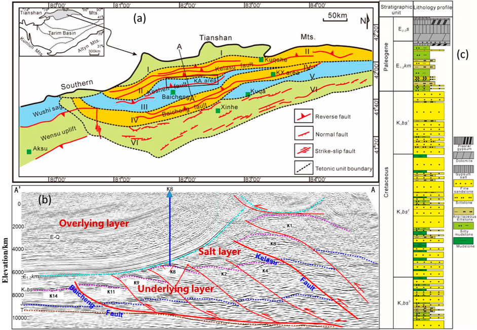
FIGURE 1. Maps show the elementary structural features of the Kuqa Depression. (A) Location of the study area (from Zhang et al., 2006),I-Northern monocline tectonic zone; II-Kelasu tectonic zone; III-Baicheng sag; IV-Qiulitage tectonic zone; V-Yangxia sag; VI-Northern Tarim Uplift; (B) Tectonic cross-section of the location shown in (A).Pre-T: Silurian to Triassic; J: Jurassic; K₁y-K₁s-K₁b: Yageliemu Formation+ Shushanhe Fromation-Baxigai Fromation; E_1-2km:Kumugeliemu Formation; E_2-3s:Suweiyizu Formation; N₁j: Jidike Formation; N₁k: Kangcun Formation; N₂k–Q₁x: Kuqa Formation to Quaternary; (C) Schematic stratigraphy of the Kuqa Depression.

3 Fracture’s characteristics and formation timing

3.1 Development characteristics of fractures

Structural fractures in the K₁bs of the Keshen gas reservoir were mainly identified and analyzed from core observation, thin section study and formation micro-imaging (FMI) interpretations. The fractures present in the six cored wells could be subdivided based on their orientation into six distinct, mutually abutting fracture sets oriented nearly EW (Set I), NNW-SSE (Set III), NE–SW (Set IV), NNE-SSW (Set V) and SN (VI) (Figure 2). Some of these shear fractures constituted three conjugate fracture systems, and the corresponding bisectors of shearing angles pointed to 310°, 347° and 13° respectively. It could be inferred from the theory of structural geology that these three orientations respectively indicated the three stages of tectonic movement from the southern margin of the Tianshan Mountains since the Cenozoic period. Observations from cores and analysis from FMI showed that the dip angle of fractures in Keshen gas reservoir mainly ranged from 75-90 (i.e., vertical fractures), followed by 45-75 (i.e., high-angle fractures) and 15-45 (i.e., low-angle fractures). Low dip-angle and horizontal fractures were almost not developed, accounting for only about 0.1% of the total number of fractures, generally located in the limb and saddle areas of the anticline. The statistical results showed that the macrofracture apertures after correction mainly ranged from 0.1 to 0.4 mm, except for some fractures in the eastern anticline exceeding 0.69 mm. As a result of geological paleo-fluid action (Olson et al., 2009), most fractures in K₁bs were unfilled and semi-filled, in which the filled fractures accounted for less than half of the total (approximately 27%), with anhydrite and dolomite as the main fillings. Macroscopically, the strong deformation of the high part of the anticline made the fracture aperture relatively large and the filling degree low, thus making the high part of the anticline a high-yield area of natural gas. For example, the absolute open flow (AOF) of single wells in the high part of Keshen anticline reached 397×10⁴–523×10⁴ m³/d, while the productivity in the limbs were relatively poor and the relative AOF was only 272×10⁴–328×10⁴ m³/d.

FIGURE 2

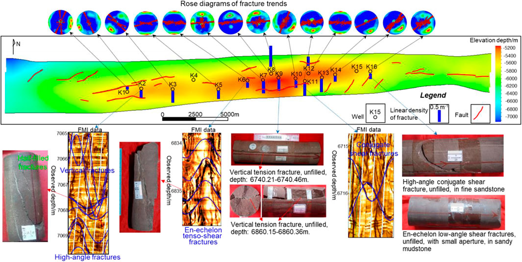
FIGURE 2. Characteristics of structural fractures observed in drill cores and FMI of Kehsen reservoir.

The structural fractures most frequently encountered in the reservoir of the area were planar discontinuities that are sub-perpendicular to the bedding and can be divided into three basic types namely tension fracture, tenso-shear fracture, and shear fracture, respectively accounting for 67%, 17%, 16% of the total number of fractures. As an important indicator for revealing the development degree of fractures in reservoirs, the fracture density can be divided into linear density (D_lf), areal density (D_sf) and volume density (D_vf). Among the three, the D_lf is defined as the number of fractures per unit length, which is a kind of parameter that can most directly and effectively characterize the fracture development degree (Golf-Racht, 1982; Ju et al., 2014). The results from core observations and FMI interpretations suggested that, the average D_lf of fractures in K₁bs mainly ranged from 0.2 m⁻¹ to1.2 m⁻¹, showing strong differences and heterogeneity both in plane and vertical. For example, fractures were the most developed in siltstone, with a linear density of ∼1.52 m⁻¹, followed by fine sandstone and medium sandstone, with a D_lf of 1.01 m⁻¹ and 0.61 m⁻¹, respectively. In contrast, fractures were not developed in mudstone, and the D_lf was generally below 0.51 m⁻¹. Structurally, the fracture D_lf of the high parts of the anticline was obviously higher than that of the low part and higher than that of the limb. The average fracture density at the eastern highs of the Keshen anticline reached 1.19 m⁻¹, which was significantly higher than that at the western highs (0.61 m⁻¹) (Figure 2).

3.2 Generation timing of fractures

Currently, rock AE test and structural trace analysis are the most common and effective techniques for determining paleo-tectonic stress value and fracture formation period. Combining previous studies and the results of this analysis, it is concluded that since the late Cretaceous three regional tectonic movements in Kuqa depression and Keshen gas reservoir are recorded, i.e., the Late Yanshanian-Early Himalayan period, the middle and late Himalayan movements, which controlled the development of a series of folds, faults and fractures (Zhang et al., 2020; Zhao et al., 2021). The early Cretaceous strata encountered four paleo-tectonic movements after eliminating the influence of current tectonic movements from acoustic emission (AE) tests (Figure 3). The Paleogene and Neogene strata recorded three and two paleo-tectonic movements, respectively. Furthermore, referring to the regional tectonic background, the two major paleo-tectonic movements expressed by Neogene rocks correspond to the tectonic movements in the middle and late Himalayan periods, while the other two major tectonic movements correspond to the early Himalayan and late Yanshanian tectonic movements, respectively.

FIGURE 3

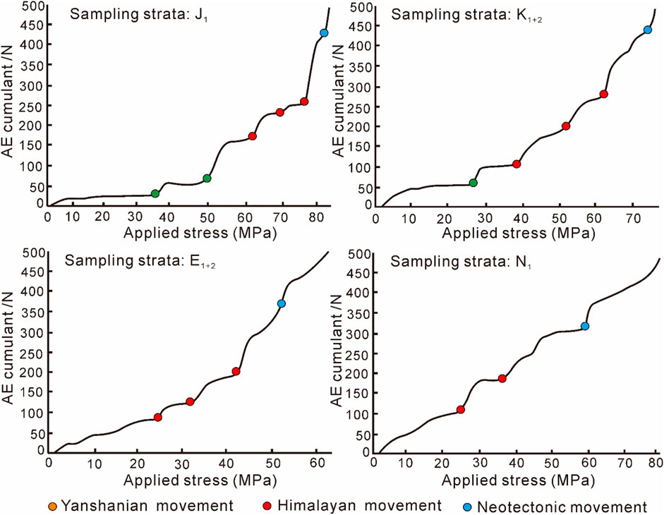
FIGURE 3. Typical response curves of AE experiment of rocks in different formations of Keshen gas reservoir (Note that this is only part of the data).

Furthermore, the combination of Andersonian faulting modes and Geomechanics Theory can effectively analyze the formation stage and time problems of complex fracture networks. As shown in Figure 2, nearly 6,000 fracture data from FMI and cores indicated that the number of NW-trending fractures account for 52.18% of the total and the NE-trending fractures account for about 35.1%. In contrast, the number of nearly EW-trending fractures account for approximately 9.78% of the total number, while the nearly SN-trending fractures account for only 2.93%. In the Kuqa depression, both the statistical results of folds, faults, conjugate joints and the experimental results of rock AE shows that the maximum principal compressive stress of paleotectonic stress field during the late Yanshan movement to Himalayan movement is nearly SN-trending (specifically, ∼NNW350°). However, a series of en-echelon faults had been developed in Keshen gas field, which is a secondary structural unit in the Kuqa depression, indicating that there existed a local torsional stress field at the same time (Figure 2). In other words, the major faults on the boundary of Keshen gas field experienced left-lateral and right-lateral shear movements during the Himalayan movements, which caused the change of fracture orientation on the plane. It can be inferred from the above that, in the late Yanshanian and early Himalayan periods, a series of nearly EW-trending tensile fractures were mainly developed in the Keshen area under the environment of long-term weak extension and short-term weak compression (Figure 4). During the middle Himalayan period, the anticline was initially in shape under the strong compression and local left-lateral shear stress field. In the Keshen area, some NE-trending conjugate fractures and a small amount of nearly EW- trending tensile fractures were formed. In the initial folded framework, the anticline was strongly uplifted and an obvious tensile stress environment appeared at the top due to the combined action of the strong compression of the Tianshan Mountains and the dextral stress field of the boundary fault. With this information, only a series of conjugated fractures developed on the limbs, whereas a large number of tensile fractures/faults with parallel hinges developed at the top (Figure 4).

FIGURE 4

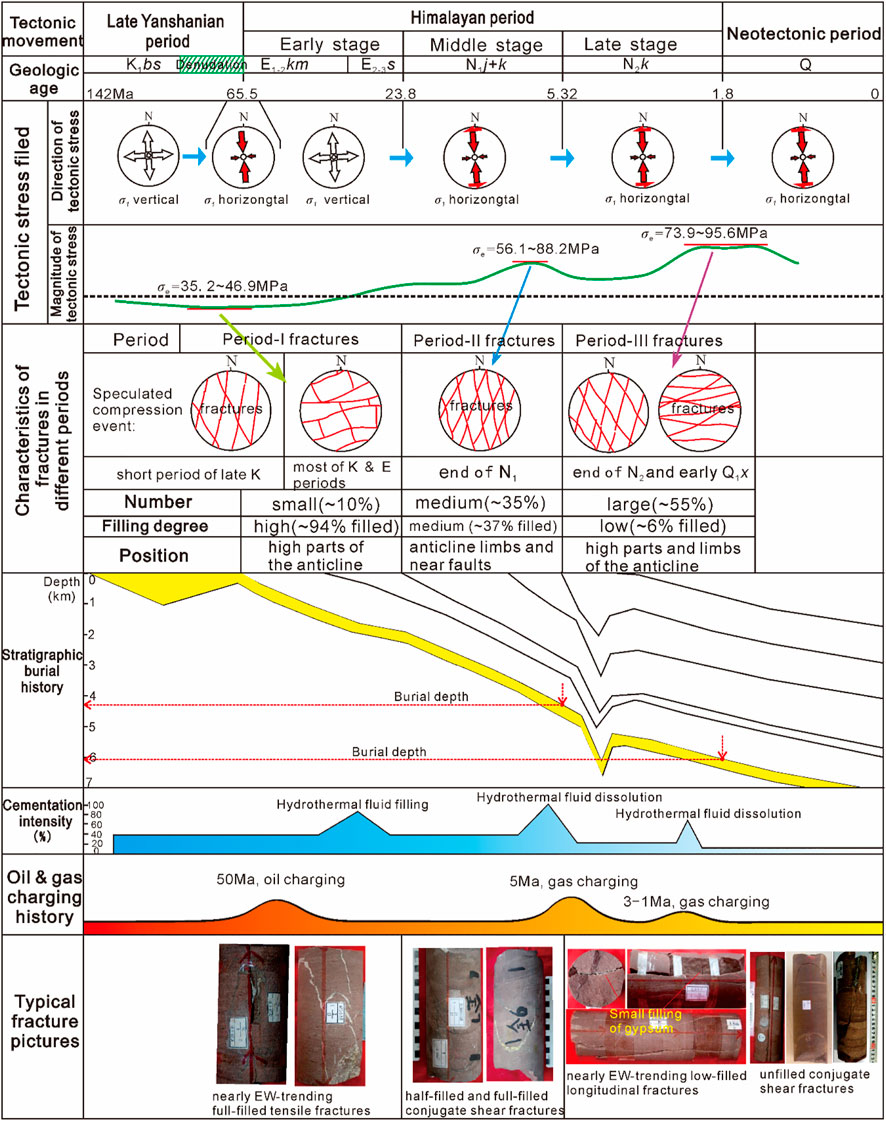
FIGURE 4. Sequence of fracture formation and cementation relative to regional tectonic events and burial history and for the Kuqa Depression. Part of the paleostress data from Zeng et al. (2004) and Li et al. (2015). And, the statistics of diagenetic cementation and fracture filling are derived from a large number of microscopic thin slices and drilling core data, respectively.

According to the results of the diagenetic evolution sequence of the reservoirs in the Keshen area, from the Late Cretaceous to the present, the diagenesis and compaction of the K₁bs reservoir has a tendency to become weaker (Li et al., 2017; Li et al., 2018). Under the influence of mantle thermal activity during the Paleogene period, a large-scale deep thermal fluid diagenetic event occurred in the Kuqa Depression and the diagenesis occurred in the early diagenetic stage-A from the epigenetic stage (Li et al., 2018). The core statistics showed that under the influence of this hydrothermal fluid diagenesis, the extensional fractures in the Keshen gas field are basically filled with calcite and gypsum, with an average filling degree of 94%. On the contrary, during Miocene to Pleistocene, the overall burial depth of the Keshen gas field increased and the storage space of reservoir was dominated by lateral and vertical compaction under strong thrust action. During this period, the reservoir reached the middle diagenetic stage-A, the deep thermal fluid was dominated by extensive acid dissolution and the porosity of the fractures developed during the same period increased. However, due to the existence of the overlying Paleogene gypsum-salt layer, a large amount of anhydrite and dolomite minerals were transported into the K₁bs reservoir under the action of stratum water, making some fractures partially filled (Figure 4). It can be seen that for the exploration and development of the Keshen gas field, the structural fractures developed in the middle and late Himalayan Movement are effective and also the focus of our research.

4 Methods and theory

4.1 Simulation of multistage paleotectonic stress field

4.1.1 Establishment of geological model

An accurate and reasonable 3D geological model (e.g., paleo-tectonic model) is crucial to numerical simulation of tectonic stress field and fractures. Generally, horizon data and fault data related to geological and geomechanical models were derived from the interpretation of the post-stack 3D seismic data (Figures 5A,B). The traditional corner grid modeling process, may lead to drastic changes in the thickness of the same small layer and even unreasonable interleaving between layers. Therefore, a deterministic modelling method was used to establish the geological model of the study area based on the corner point gridding (Figure 5C). After transforming the corner point grid model into key points, a finite element (FE) model close to the real underground geological structure was established the in the ANSYS software. In detail, the construction of 3D geologic model incorporated three horizons of K₁bs¹, K₁bs², K₁bs³ or several isolated blocks (Figures 5A,B). Since there were few wells drilled in the K₁bs³ and the geological stratification data were relatively scarce, K₁bs³ can only be combined into a set of strata in modeling. As a result, the average thickness of six layers K₁bs^1-1, K₁bs^1-2, K₁bs^2-1, K₁bs^2-2, K₁bs^2-3 and K₁bs³ within geologic model was set to 25 m, 25 m, 70 m, 40 m, 70 m and 80 m, respectively. However, due to the quality of ultra-deep seismic data, the reliability of some low-order faults in Keshen anticline is debatable. In this study, by combining the comparison and verification of various seismic attributes, such as original seismic amplitude volume, maximum positive curvature attribute, variance attribute, and ant tracking attribute, 12 relatively reliable large-scale faults were retained for geological modeling among the 23 originally interpreted faults.

FIGURE 5

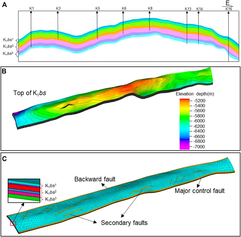
FIGURE 5. (A) Horizon model of post-stack seismic interpretation; (B) 3D geological model based on corner point grid; (C) Simplified 3D FE models of the Bashenjiqike Formation in the Keshen gas reservoir.

4.1.2 Geomechanical modelling

Rock mechanics parameters are key parameters characterizing the degree of formation brittleness and possible fracture development. Two methods can be used to obtain rock mechanics parameters: rock mechanical experiments on core samples or calculation of well logging curves. The former obtains the static mechanical parameters of rock, while the latter obtains the dynamic parameters with large errors between them. Therefore, it is necessary to construct the correlation between them based on laboratory data. In this study, conventional uniaxial and triaxial compression tests were conducted to obtain static rock mechanical parameters. A total of 48 rock samples were drilled from K₁bs Formation, involving different lithology and horizons to ensure the rationality and practicability of the data. All samples were processed according to International System for Rock Mechanics (ISRM)-suggested methods with a core diameter of 25 mm and length of 50mm, ends ground flat to 0.01 mm with vertical deviation of less than 0.25°. In order to meet the underground formation conditions and consider the safety problems, the confining pressures during the Triaxial experiments could be set to 35 MPa, 45 MPa, and 55 MPa, respectively, and the loading rate could be set to 0.01 mm/s. In this way, the complete stress-strain curves and mechanical parameters of sandstone were acquired, including the uniaxial/triaxial compression strength or peak strength (σ_c), Young’s modulus (E) and Poisson’s ratio (μ), cohesive strength (C₀) and friction angle (φ). Prior to this, corrections should be made between uniaxial and triaxial experimental data, i.e., uniaxial results are corrected to triaxial conditions and then used to calibrate the log calculation results (Figure 6) to determine the relationship between log dynamic parameters and triaxial static parameters. Based on the corrected triaxial test data, the dynamic-static relationship of rock mechanical parameters can be obtained by further modifying the depth of rock samples, as shown below:

$\{\begin{array}{c}{\mathrm{E}}_{\mathrm{t}\mathrm{s}}=0.125·{\mathrm{E}}_{\mathrm{t}\mathrm{d}}+7.8215,\mathrm{R}=0.728\\ {\mathrm{U}}_{\mathrm{t}\mathrm{s}}=3.968·{\mathrm{U}}_{\mathrm{t}\mathrm{d}}-0.7551,\mathrm{R}=0.855\end{array}(1)$

where, E_ts is the triaxial static Young’s modulus; E_td is the triaxial dynamic Young’s modulus; U_tsis the triaxial static Poisson’s ratio; U_td is the triaxial dynamic Poisson’s ratio; R is the correlation coefficient. By using the continuous logging interpretation method and combining the above dynamic-static relationship, the triaxial static mechanical parameters of multiple wells can be calculated, and the average value of six sand groups in K₁bs can be obtained as the basis for numerical simulation.

FIGURE 6

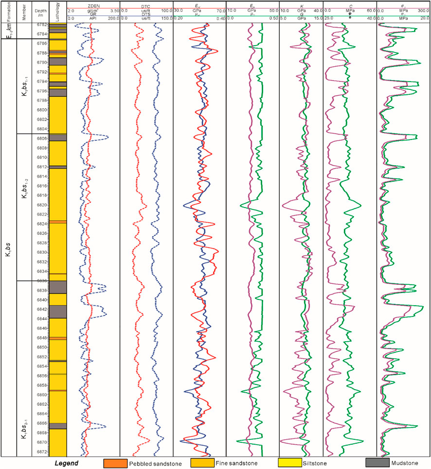
FIGURE 6. Comprehensive columnar section of rock mechanics parameters in the K₁bs of the K15 well. Here, ZDEN is the litho-density logging, GR is the natural gamma logging, DTC is the P-wave time difference logging, DTS is the S-wave time difference logging, E_td is the dynamic Young’s modulus of rock, μ_td is the dynamic Poisson’s ratio of rock, E_td is the corrected static Young’s modulus of rock, μ_ts is the corrected static Poisson’s ratio of rock, K is the bulk modulus of rock, and K =E/[3 × (1-2μ)], G is the shear modulus of rock, and G =E/[2 × (1 + μ)], φ is the internal friction angle of rock, σ_c is the compressive strength of rock; σt is the tensile strength of rock.

The mechanical parameters of the fault zone directly affect the numerical simulation results, which is the basis of modeling (Liu et al., 2017). Before the formation of faults or folds, the overall Young’s modulus was about 115–135% of the sedimentary strata in the model, while the Poisson’s ratio was the opposite whereas the faults correspond to the weak zones after the formation. According to the above dynamic-static correction results, the average static Young’s modulus, Poisson’s ratio, rock cohesion, internal friction angle, bulk modulus of rock, and shear modulus of each geological unit were summarized as shown in Figure 6 and Table 1.

TABLE 1

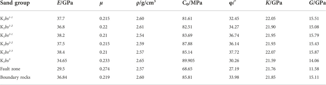
TABLE 1. Average mechanical properties of the K₁bs tight sandstones from triaxial compressional tests. In the table, E is the rock Young’s modulus; μ is the Poisson’s ratio; σ_c is the rock compressive strength; ρ is the rock density; φ is the rock internal friction angle; C₀ is the rock cohesion, K is the rock bulk modulus, and G is the rock shear modulus.

4.1.3 Boundary conditions

Based on the tectonic evolution, paleostress reconstruction and related tests, boundary conditions of two formation periods of fractures were defined, including the load application and displacement constraint. The determination of stress magnitude was based on the AE tests (Figure 3), and the maximum principal stress in different tectonic periods were summarized. Due to the occurrence of tectonic movements, fluids generally exists in the formations, that is, the interaction between the pore pressure and the tectonic stress forms an effective stress field. However, the samples used for rock AE experiments do not contain fluid, so the value of the paleo-maximum principal stress obtained by the experiment is an effective paleostress value. Consequently, in Kuqa Depression, the tectonic stress intensity from the late Yanshanian to early Himalayan was relatively weak, located in range of 35.2–46.9 MPa. In contrast, the tectonic stress intensity of the middle Himalayan movement at the end of the Paleogene became stronger, reaching 56.1–88.2 MPa (Figure 3, Figure 4). When entering the late Himalayan and Neotectonic period, the tectonic stress intensity reached its peak, located in the range of 73.9–95.6 MPa. According to the Mohr-Coulomb strength criterion, the horizontal compression force of less than 100 MPa under deep formation conditions are not enough to generate so many high-angle structural fractures, which cannot be directly used for FE numerical simulation. As showed in Figure 4, during the middle Himalayan, the burial depth of the top of K₁bs formation was ∼−4,250 m, and the corresponding vertical stress (i.e., σ_v) reached 108 MPa. In contrast, under the strong compression in the late Himalayan period, the burial depth of the top surface of K₁bs reached ∼-6,100 m, and the corresponding vertical stress reached 155 MPa.

Since most of the wells in Keshen gas field are located at the top of an anticline, in terms of Andersonian faulting and Mohr-Coulomb theory, a series of sub-vertical shear fractures (as shown by core observation results) can only be developed under the Type-III stress environment (i.e.,σ_H>σ_v>σ_h). It can be inferred that in the middle and late Himalayan movements, only when the horizontal tectonic stress exceeded 108 MPa or 155 MPa can the Type-III stress state be satisfied. According to the AE experiment results and the concept of equivalent paleo-stress, a reasonable boundary condition scheme for the Keshen model was finally determined after repeated attempts. For the middle Himalayan model, pressures of approximately 140 MPa and 65 MPa were applied on the north and east-west sides, respectively, and 20 MPa of sinistral shear stress was applied on the east-west boundary (Figure 7A). For the late Himalayan model, pressures of approximately 180 MPa and 85 MPa were applied on the north and east-west sides, respectively, and 40 MPa of dextral shear stress was applied on the east-west boundary (Figure 7B). For these two models, the southern edge was set as a fixed boundary to appropriately reflect the blocking effect of the South Tarim Basin. Simultaneously, the bottom boundary of the model was also fixed and gravity load was automatically applied by the software, to maintain the system in equilibrium.

FIGURE 7

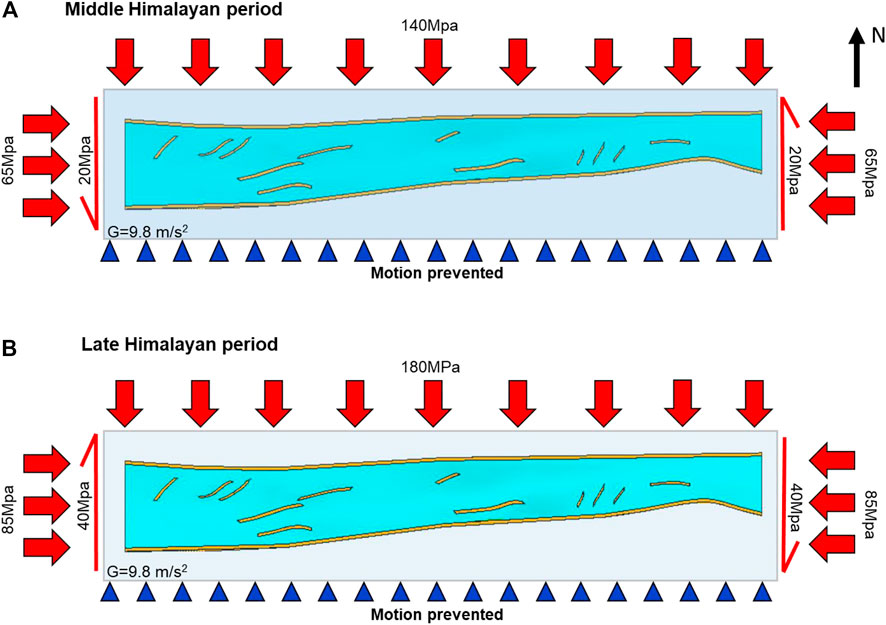
FIGURE 7. Mechanical model of tectonic stress field simulation of study area. (A) Boundary condition in middle Himalayan period; (B) Boundary condition in late Himalayan period.

The deformation and destruction of geological structures, especially the uplift of folds, occurs under the action of long-term tectonic movements and is no longer a simple elastic mechanics problem. The general-purpose elastic-plastic FE method based on ANSYS software was selected for this study. This software is well-suited for analyzing large-deformation problems in geomechanics over a wide range of scales in one, two, and three dimensions (Smart et al., 2012; Kim et al., 2015; Ass & Mat, 2021; Tojaga et al., 2021). In order to eliminate the boundary effect of the stress field simulation as much as possible, it was necessary to nest a larger rectangular parallelepiped outside the Keshen geologic model with planar area of ∼1.5 times (Figure 7). The geomechanical model was segmented using a triangular mesh, allowing a large number of elements and nodes to be subdivided. Particularly, the meshing of the target layer and fault zone needed to be much finer than that of the surrounding rock. The geologic models of middle and late Himalayan periods were finally divided into 34,577 nodes, 129,576 elements and 46,327 nodes, 199,846 elements respectively.

4.2 Calculation of fracture linear density

4.2.1 Rock constitutive model

According to the theory of minimum energy dissipation, the material or rock failure process always occurs in the weakest place and in the most destructible way, that is, the theory of minimum energy dissipation rate is always satisfied in the energy consumption process (Luo et al., 2009; Leykin, 2015).

Following the damage mechanics theory, the continuous damage variable D (0 ≦ D ≦1) can be used to directly measure the damage degree of rock mass (Luo et al., 2009). Essentially, the damage of brittle rock is an energy-consuming process under the action of load, which should also be constrained by the principle of minimum energy consumption. In the process of rock failure or energy dissipation, the infinite small unit will produce irreversible strain ${\epsilon }_i\left(i=\mathrm{1,2,3}\right)$ before reaching complete destruction. If other factors were not considered, and the principal strain ${\epsilon }_i$ caused by the force was regarded as the only energy dissipation mechanism of the rock mass in failure process, the corresponding expression of the energy dissipation rate is as follows (Li, 2011; Peng et al., 2016):

$\phi ={\sigma }_i\bullet \dot{{\epsilon }_i}(\mathrm{1a})$

where, $\phi$ is the energy dissipation rate (J/s); ${\sigma }_i\left(i=\mathrm{1,2,3}\right)$ are the three principal stress (MPa); $\dot{{\epsilon }_i}\left(i=\mathrm{1,2,3}\right)$ are the three strain rate tensor (s⁻¹).

Combined with the generalized Hooke’s law including the damage variable $D$, the irreversible strain rate tensor $\dot{{\epsilon }_i}$ was obtained using the formula below:

$\{\begin{array}{c}\dot{{\epsilon }_1}=-\frac{\dot{D}}{{\left[1-D\right]}^{2}E}\left[{\sigma }_1-\mathrm{\mu }\left({\sigma }_2+{\sigma }_3\right)\right]\\ \dot{{\epsilon }_2}=-\frac{\dot{D}}{{\left[1-D\right]}^{2}E}\left[{\sigma }_2-\mathrm{\mu }\left({\sigma }_1+{\sigma }_3\right)\right]\\ \dot{{\epsilon }_3}=-\frac{\dot{D}}{{\left[1-D\right]}^{2}E}\left[{\sigma }_3-\mathrm{\mu }\left({\sigma }_1+{\sigma }_2\right)\right]\end{array}(2)$

Substituting equation (2) into equation (1), the energy consumption rate expression is shown below:

$\phi =-\frac{\dot{D}}{{\left[1-D\right]}^{2}E}\left[{\sigma }_1^2+{\sigma }_2^2+{\sigma }_3^2-2\mathrm{\mu }\left({\sigma }_1{\sigma }_2+{\sigma }_2{\sigma }_3+{\sigma }_1{\sigma }_3\right)\right](3)$

where, $\phi$ is the energy dissipation rate (J/s); $D$ is the damage variable; $\dot{D}$ is the damage rate; $E$, μ are the elastic modulus (GPa) and Poisson’s ratio of the rock mass before failure, and the values could be measured by experiments; ${\sigma }_i\left(i=\mathrm{1,2,3}\right)$ are the three principal stress (MPa); $\dot{{\epsilon }_i}\left(i=\mathrm{1,2,3}\right)$ are the three strain rate tensor (s⁻¹).The unified energy yield criterion for rock expresses the relationship between shear strain energy and volumetric strain energy and can be used as a constraint condition for the process of rock damage and energy dissipation (Sun et al., 2018), so the constraint under triaxial stress conditions are as below:

$F\left({\sigma }_1,{\sigma }_2,{\sigma }_3\right)=\frac{1}{2G}{\left[\frac{{\sigma }_1-{\sigma }_2}{{2\mathit{cos}\phi }_{12}}-\frac{\left({\sigma }_1+{\sigma }_2\right)}{2}{\mathit{tan}\phi }_{12}\right]}^2+\frac{1}{2G}{\left[\frac{{\sigma }_2-{\sigma }_3}{{2\mathit{cos}\phi }_{23}}-\frac{\left({\sigma }_2+{\sigma }_3\right)}{2}{\mathit{tan}\phi }_{23}\right]}^2+\frac{1}{2G}{\left[\frac{{\sigma }_1-{\sigma }_3}{{2\mathit{cos}\phi }_{13}}-\frac{\left({\sigma }_1+{\sigma }_3\right)}{2}{\mathit{tan}\phi }_{13}\right]}^2+\alpha \frac{{\left({\sigma }_1+{\sigma }_2+{\sigma }_3\right)}^2}{18K}+\beta (4)$

where, $\alpha$ and $\beta$ are material parameters that characterize the relationship between shear strain energy and volumetric deformation energy during rock yield; φ₁₂, φ₂₃, φ₁₃ are the internal friction angles of rock (º); G and K are the bulk modulus and shear modulus (GPa) respectively. The above parameters can be measured experimentally.

According to the minimum energy consumption theory (Tabarrok & Leech, 2002), in the damage evolution process of rock, the consumption rate has the stationary value under the corresponding conditions. Therefore, Lagrange multiplier was introduced and the following expression was obtained:

$\{\begin{array}{c}\frac{\partial \left(\phi +\lambda F\right)}{{\partial \sigma }_1}=0\\ \frac{\partial \left(\phi +\lambda F\right)}{{\partial \sigma }_2}=0\\ \frac{\partial \left(\phi +\lambda F\right)}{{\partial \sigma }_3}=0\end{array}(5)$

Combining formulas (Eqs 1–5, the rock damage equation under triaxial condition is expressed as:

$D=1-\mathit{exp}\left[\frac{\lambda A}{2\left({\epsilon }_1+{\epsilon }_2+{\epsilon }_3\right)}+C_0\right](6)$

and

$\dot{D}=-\frac{\lambda A}{2\left({\epsilon }_1+{\epsilon }_2+{\epsilon }_3\right)}\mathit{exp}\left[\frac{\lambda A}{2\left({\epsilon }_1+{\epsilon }_2+{\epsilon }_3\right)}+C_0\right](7)$

As the Damage Mechanics Theory (Krajcinovic, 1989) states: when the strain reaches the threshold, the rock damage begins to develop and is in the elastic deformation stage before the damage threshold. Thus, the rock damage equation after introducing damage threshold strain ${\epsilon }_0$ is:

$D=\{\begin{array}{c}0,{\epsilon }_1<{\epsilon }_0\\ 1-\mathit{exp}\left[\frac{\lambda A}{2\left({\epsilon }_1+{\epsilon }_2+{\epsilon }_3\right)}+C_0\right],{\epsilon }_1\ge {\epsilon }_0\end{array}(8)$

where, $A=\frac{E}{4G}\left[\frac{{\left(1-\mathit{sin}{\phi }_{12}\right)}^2}{{\left(\mathit{cos}{\phi }_{12}\right)}^2}+\frac{{\left(1-\mathit{sin}{\phi }_{13}\right)}^2}{{\left(\mathit{cos}{\phi }_{13}\right)}^2}-\frac{1}{2G}+\frac{\alpha }{3K}\right]{\epsilon }_1+\frac{1}{4G}\left[\frac{{\left(1+\mathit{sin}{\phi }_{12}\right)}^2{+\mu \left(1-\mathit{sin}{\phi }_{12}\right)}^2}{{\left(\mathit{cos}{\phi }_{12}\right)}^2}+\frac{{\left(1-\mathit{sin}{\phi }_{23}\right)}^2}{{\left(\mathit{cos}{\phi }_{23}\right)}^2}+\frac{\mu {\left(1-\mathit{sin}{\phi }_{13}\right)}^2}{{\left(\mathit{cos}{\phi }_{13}\right)}^2}\right]{\sigma }_2+\frac{1}{4G}\left[\frac{{\left(1-\mathit{sin}{\phi }_{12}\right)}^2}{{\left(\mathit{cos}{\phi }_{12}\right)}^2}+\frac{{\left(1+\mathit{sin}{\phi }_{23}\right)}^2}{{\left(\mathit{cos}{\phi }_{23}\right)}^2}+\frac{{\left(1+\mathit{sin}{\phi }_{13}\right)}^2+\mu {\left(1-\mathit{sin}{\phi }_{13}\right)}^2}{{\left(\mathit{cos}{\phi }_{13}\right)}^2}\right]{\sigma }_3+\left(-\frac{1}{2G}+\frac{\alpha }{3K}\right)\left(\mu +1\right)\left({\sigma }_2+{\sigma }_3\right)$; λ and C₀ were the constants related to lithology. Therefore, combined with the generalized Hooke’s law containing damage variables, the constitutive model of rock was obtained:

${\sigma }_t=\{\begin{array}{c}E{\epsilon }_1+\mu {\sigma }_2+\mu {\sigma }_3,{\epsilon }_1<{\epsilon }_0\\ E{\epsilon }_1\mathit{exp}\left[\frac{\lambda A}{2\left({\epsilon }_1+{\epsilon }_2+{\epsilon }_3\right)}+C_0\right]+\mu {\sigma }_2+\mu {\sigma }_3,{\epsilon }_1\ge {\epsilon }_0\end{array}(9)$

4.2.2 Rock failure criterion

The previous experimental results show that when the axial stress reaches 0.75, 0.85 and 0.92 times the peak strength, a large number of micro-cracks in the brittle rock begin to expand and connect (Eberhardt et al., 1998; Dai et al., 2011; Ju et al., 2017). Finally, macroscopic fractures are formed at the peak strength, followed by slipping along the fracture planes to form faults (Gudmundsson, 2010). Therefore, using the peak point of the stress-strain curve to identify the model parameters can make the parameters have clear physical meanings for the deep tight sandstone with strong brittle characteristics. Assuming that the stress and strain at the peak point of stress-strain curve under confining pressure were σ_1s, σ_2s, σ_3s, Ɛ_1s, Ɛ_2s, Ɛ_3s, respectively, then there were:

$\frac{d{\sigma }_t}{d{\epsilon }_1}=0(10)$

The formula (6) was arranged and substituted into the peak condition to obtain the values of constants λ $\mathrm{a}$ nd C₀:

$\{\begin{array}{c}\lambda =\frac{2{\left({\epsilon }_{1s}+{\epsilon }_{2s}+{\epsilon }_{3s}\right)}^2}{A_0{\epsilon }_{1s}}\\ C_0=\mathit{ln}\left[{\sigma }_{1s}-\mu {\sigma }_{2s}-\mu {\sigma }_{3s}\right]-\mathit{ln}\left[E{\epsilon }_{1s}\right]-A_0\left({\epsilon }_{1s}+{\epsilon }_{2s}+{\epsilon }_{3s}\right)\end{array}(11)$

The damage threshold could also be obtained as follows:

${\epsilon }_0=-\frac{\lambda A_0}{2C_0}-{\epsilon }_{2s}-{\epsilon }_{3s}(12)$

where, $A_0=E/4G\left[{\left(1-\mathit{sin}{\phi }_{12}\right)}^2/{\left(\mathit{cos}{\phi }_{12}\right)}^2+{\left(1-\mathit{sin}{\phi }_{13}\right)}^2/{\left(\mathit{cos}{\phi }_{13}\right)}^2-1/2G+\alpha /3K\right]{\epsilon }_{1s}+1/4G\left[{\left(1+\mathit{sin}{\phi }_{12}\right)}^2{+\mu \left(1-\mathit{sin}{\phi }_{12}\right)}^2/{\left(\mathit{cos}{\phi }_{12}\right)}^2+{\left(1-\mathit{sin}{\phi }_{23}\right)}^2/{\left(\mathit{cos}{\phi }_{23}\right)}^2+\mu {\left(1-\mathit{sin}{\phi }_{13}\right)}^2/{\left(\mathit{cos}{\phi }_{13}\right)}^2\right]{\sigma }_{2s}+1/4G\left[{\left(1-\mathit{sin}{\phi }_{12}\right)}^2/{\left(\mathit{cos}{\phi }_{12}\right)}^2+{\left(1+\mathit{sin}{\phi }_{23}\right)}^2/{\left(\mathit{cos}{\phi }_{23}\right)}^2+{\left(1+\mathit{sin}{\phi }_{13}\right)}^2+\mu {\left(1-\mathit{sin}{\phi }_{13}\right)}^2/{\left(\mathit{cos}{\phi }_{13}\right)}^2\right]{\sigma }_{3s}+\left(-1/2G+\alpha /3K\right)\left(\mu +1\right)\left({\sigma }_2+{\sigma }_{3s}\right).$ From above we could get:

${\phi }_0=\left[E{\epsilon }_0\mathit{exp}\left[\frac{\lambda A_0}{2\left({\epsilon }_1+{\epsilon }_2+{\epsilon }_3\right)}+C_0\right]+\mu {\sigma }_2+\mu {\sigma }_3\right]{\epsilon }_0(13)$

Finally, the consumption rate expression under the framework of minimum energy consumption principle could be obtained:

$\phi =\{\begin{array}{c}\left(E{\epsilon }_1+\mu {\sigma }_2+\mu {\sigma }_3\right){\epsilon }_1,{\epsilon }_1<{\epsilon }_0\\ \left(E{\epsilon }_1\mathit{exp}\left[\frac{\lambda A}{2\left({\epsilon }_1+{\epsilon }_2+{\epsilon }_3\right)}+C_0\right]+\mu {\sigma }_2+\mu {\sigma }_3\right){\epsilon }_1,{\epsilon }_1\ge {\epsilon }_0\end{array}(14)$

It can be seen from the formula that when $\phi >{\phi }_0$, the rock lost its steady state and broke, that is, the tensile fracture or shear fracture was formed.

4.2.3 Geomechanical models of fracture parameters

4.2.3.1 Fracture dip angle

As shown in Figure 8, under the principal stress coordinate system with the coordinate origin as the pole and the positive semi-axis of the maximum principal stress as the polar axis, the appropriate polar coordinate system was established. The angle between the fracture surface and the maximum principal stress was the rupture angle. First, the stress function expression F (r, θ) of fracture surface (r, θ) point needed to be determined (Peng et al., 2019), that is:

$F=r^2\left(\mathit{acos}2\theta +bsin2\theta +c\theta +d\right)(15)$

where, a, b, c and d were arbitrary constants. After substituting it into the equation $\left(\frac{{\partial }^2}{{\partial r}^2}+\frac{1}{r}\frac{\partial }{\partial r}+\frac{1}{r^2}\frac{{\partial }^2}{{\partial \theta }^2}\right)\phi =0$, it was found that this function satisfied the compatibility equation. Therefore, the stress component can be expressed as (Peng et al., 2020):

$\{\begin{array}{c}{\sigma }_r=\frac{1}{r}\frac{\partial F}{\partial r}+\frac{1}{r^2}\frac{{\partial }^{2}F}{\partial {\theta }^2}=-2\left(\mathit{acos}2\theta +bsin2\theta -c\theta -d\right)\\ {\sigma }_{\theta }=\frac{{\partial }^{2}F}{\partial r^2}=2\left(\mathit{acos}2\theta +bsin2\theta +c\theta +d\right)\\ {\tau }_{r\theta }=-\frac{\partial }{\partial r}\left(\frac{1}{r}\frac{\partial F}{\partial \theta }\right)=2\mathit{asin}2\theta -2bcos2\theta -c\end{array}(16)$

where, ${\sigma }_r$ and ${\sigma }_{\theta }$ are the stress components along both radial and annular directions in polar coordinate systems (MPa); ${\tau }_{r\theta }$ is the shear stress component in polar coordinate system (MPa).

FIGURE 8

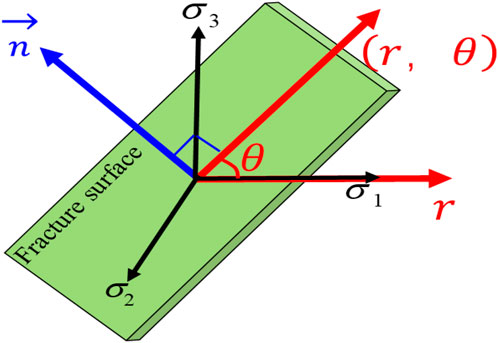
FIGURE 8. Diagram of calculating the fracture angle in polar coordinate system.

Next, substitute (Eq. 16) into the boundary conditions:

If $\theta =0°$, $\{\begin{array}{c}{\sigma }_r=0\\ {\tau }_{r\theta }=0\end{array}$, if $\theta =90°$, $\{\begin{array}{c}{\sigma }_r=-{\sigma }_{\mathit{max}}\\ {\tau }_{r\theta }=0\end{array}$ (17)Where, ${\sigma }_{\mathit{max}}$ is the maximum principal stress (MPa).

Thus, the corresponding values of the constants a, b, c, and d were obtained, namely:

$\{\begin{array}{c}a=d=-\frac{{\sigma }_{\mathit{max}}}{4}{r}^2\\ b=c=0\end{array}(18)$

At the same time, the stress function expression could be expressed as:

$F=-\frac{{\sigma }_{\mathit{max}}}{4}{r}^4\mathit{cos}2\theta -\frac{{\sigma }_{\mathit{max}}}{4}{r}^4(19)$

Further combined with Eq. 2, the energy consumption rate expression in the polar coordinate system was obtained:

$\phi =-\frac{\dot{D}}{{\left(1-D\right)}^{2}E}{\left(-\frac{{\sigma }_{\mathit{max}}}{4}\mathit{cos}2\theta -\frac{{\sigma }_{\mathit{max}}}{4}\right)}^2(20)$

Finally, the rupture angle expression obtained by the minimum energy dissipation principle was:

$\theta =\frac{1}{2}\mathit{arccos}\left[\sqrt{\frac{16E\phi {\left(1-D\right)}^2}{\dot{D}{\sigma }_{\mathit{max}}^2}}-1\right](21)$

where$:D=1-\mathit{exp}\left[\frac{\lambda A}{2\left({\epsilon }_1+{\epsilon }_2+{\epsilon }_3\right)}+C_0\right]$; $\dot{D}=-\frac{\lambda A}{2\left({\epsilon }_1+{\epsilon }_2+{\epsilon }_3\right)}\mathit{exp}\left[\frac{\lambda A}{2\left({\epsilon }_1+{\epsilon }_2+{\epsilon }_3\right)}+C_0\right].$

(2) Fracture linear density

For a brittle material such as deep tight sandstone, when the stress state reaches its failure strength, the rock will break to produce macroscopic fractures and release energy (Gdoutos, 2012; Kravchenko et al., 2014). Combined with (Eq. 14), the dissipated energy in the process of crack formation can be derived (assuming that the initial phase energy dissipation is 0):

$\omega =\int \phi dt=\int \left\{\left(E{\epsilon }_1\mathit{exp}\left[\frac{\lambda A}{2\left({\epsilon }_1+{\epsilon }_2+{\epsilon }_3\right)}+C_0\right]+\mu {\sigma }_2+\mu {\sigma }_3\right){\epsilon }_1\right\}dt=\frac{2E{\epsilon }_1^2\left({\epsilon }_1+{\epsilon }_2+{\epsilon }_3\right)}{\lambda A}\mathit{exp}\left[\frac{\lambda A}{2\left({\epsilon }_1+{\epsilon }_2+{\epsilon }_3\right)}+C_0\right]+\mu {\epsilon }_1\left({\sigma }_2+{\sigma }_3\right)-\frac{2E{\epsilon }_1^2\left({\epsilon }_1+{\epsilon }_2+{\epsilon }_3\right)}{\lambda A}{e}^{C_0}(22)$

where, $\omega$ is the strain energy released by new fractures (J); t is the moment of stress applied (s).

Generally, brittle macro-fractures occur with strain energy releasing, especially when the surrounding three-dimensional stress state reaches the rock’s strength. At this time, part of the strain energy will be released as the surface energy of the new fractures while the rest will be released in the form of elastic waves (Barton et al., 1977). Nonetheless, compared with the fracture surface energy, elastic wave energy was so weak that it can be neglected. We assume that all of the fractures in this study were caused by the releasing energy and therefore, the law of conservation of energy must be satisfied:

$\omega ={\omega }_{s}V=SJ(23)$

where $\omega$ is the strain energy released by new fractures (J); ${\omega }_s$ is the strain energy density of the new fracture surface area (J/m³); V is the unit cell volume (m³); S is the surface area of the new fractures (m²); J is the energy per unit area required for fractures, i.e., fracture surface energy (here, this energy was different from and had a far lower value than the theoretical value of molecular dissociation).

Further transformation of Eq. 23, the fracture density expression under the theory of minimum energy consumption can be obtained by the formula below:

$D_v=\frac{S}{V}=\frac{{\omega }_s}{J}=\frac{2E{\epsilon }_1^2}{\lambda AVJ}\left({\epsilon }_1+{\epsilon }_2+{\epsilon }_3\right)\mathit{exp}\left[\frac{\lambda A}{2\left({\epsilon }_1+{\epsilon }_2+{\epsilon }_3\right)}+C_0\right]+\frac{\mu {\epsilon }_1}{VJ}\left({\sigma }_2+{\sigma }_3\right)-\frac{2E{\epsilon }_1^2}{\lambda AVJ}\left({\epsilon }_1+{\epsilon }_2+{\epsilon }_3\right)e^{C_0}(24)$

where, $D_v$ is the fracture volume density per unit volume (m²/m³). Further, combined with the fracture density formula established in the previous stage (Dai et al., 2011), the fracture linear density model under the framework of the principle of minimum energy consumption was obtained:

$D_l=\{\begin{array}{c}\frac{2D_v{L}_1{L}_3\mathit{sin}\theta \mathit{cos}\theta -L_1\mathit{sin}\theta -L_3\mathit{cos}\theta }{L_1^2{\mathit{sin}}^2\theta +L_3^2{\mathit{cos}}^2\theta },\theta \ne 0\\ D_v,\theta =0\end{array}(25)$

where, $\theta =\frac{1}{2}\mathit{arccos}\left[\sqrt{\frac{16E\phi {\left(1-D\right)}^2}{\dot{D}{\sigma }_{\mathit{max}}^2}}-1\right]$; $D_l$ is the fracture linear density (1/m); L₁, L₃ were the side length of the selecting representing element volume (m).

After establishing geomechanical models through ANSYS software, the 3D paleotectonic stress field simulation was carried out in Keshen area. Then, the rock failure criterion and geomechanical models of fracture parameters were implanted into the FE platform to predict spatial distribution of fractures. As a general principle, tectonic movement is a slow process in which stress fields and energy dissipation rates are constantly changing and fractures may occur at each stage. Therefore, the coupling effect between late stress and cracks will exist where the early fractures occur. The principle of minimum energy consumption can solve this problem, that is, reaching the condition of minimum energy consumption rate will produce new fractures.

5 Results and discussion

5.1 Paleo-tectonic stress field

As shown in Figure 9, Figures 10, 11, the maximum principal stress, minimum principal stress, and stress direction of the middle and late Himalayan periods were calculated. Generally, the distribution of the maximum principal stress (σ₁) is the main factor controlling the thrust fault and anticline deformation in the compression basin whereas the minimum principal stress (σ₃) is the main factor controlling whether there is a local tensile zone at the top of the anticline. The σ₁ during the Middle Himalayan period was generally between -200 and -64 MPa (the negative sign represents the compressive stress, the positive sign represents the tensile stress) (Figure 9), and the minimum principal stress was generally between -86 and 44 MPa (Figure 10). The high-value areas were mainly concentrated in the east and west ends and north limb of Keshen anticline and distributed around the fault core, particularly at the en-echelon faults and the tip of the faults (Figure 9A). Vertically, the values of σ₁ increased with the increase of depth, for example, the expression strength of section K₁bs³ was obviously greater than that of K₁bs² and K₁bs¹. As shown in Figure 10A, the tensile-stress zones (i.e. positive values) were concentrated in the middle and east of the study area and the top of the anticline, and distributed around the fault cores. In particular, at the high parts of central Keshen anticline, the tensile stress values reached 24 MPa, indicating a relatively strong local extensional environment. Vertically, the tensile stress at the top of the anticline was significantly higher than that at the bottom, which was consistent with the neutral surface effect of flexural folding. In contrast, in the late Himalayan period, the maximum principal stress was generally between −260 and −78 MPa, the minimum principal stress was generally between −120 and 33 MPa. Compared with the middle Himalayan tectonic stress field, the intensity of σ₁ increased, and high-value areas migrated to the east of the study area. In addition, low values of σ₁ can easily occur in the high positions of anticline core and the fault cores, which was the result of concentrated release of tectonic stress (Figure 9B). Interestingly, similar to σ₁, the positive values (i.e., tensile stress) of σ₃ were concentrated at the top of the anticline and fault cores, indicating where a large number of tensile fractures occurred (Figure 10B). Generally, the distribution of the maximum principal stress (σ₁) direction is closely related to the occurrence of the fractures. According to the simulation results, from west to east of the anticline, the direction of σ₁ changed significantly, that is, from the SN to the NE, and then to the SN and EW (Figure 11). Specifically, the direction of σ₁ varied obviously at the intersection of faults and the tip of faults, especially at the position of anticline-syncline transition. Based on seismic interpretation results, this sudden change of stress direction was basically consistent with the position of NW-trending accommodation zones which jointly affected the spatial difference of stress state and the generation of fractures in different groups.

FIGURE 9

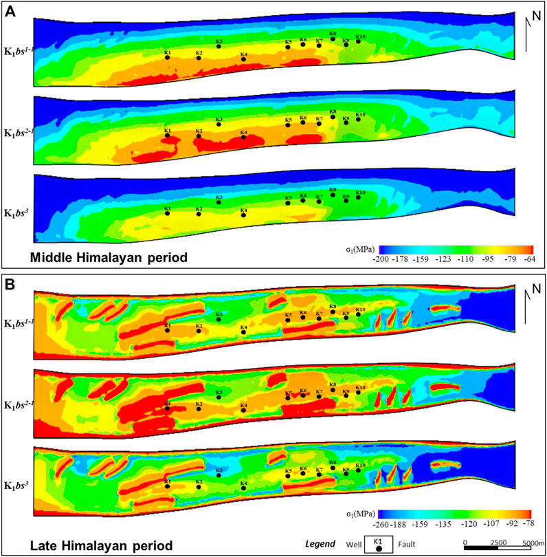
FIGURE 9. Distribution of paleo-tectonic stress field in different period. (A) Maximum principal stress in middle Himalayan period of target layer; (B) Maximum principal stress in late Himalayan period of target layer.

FIGURE 10

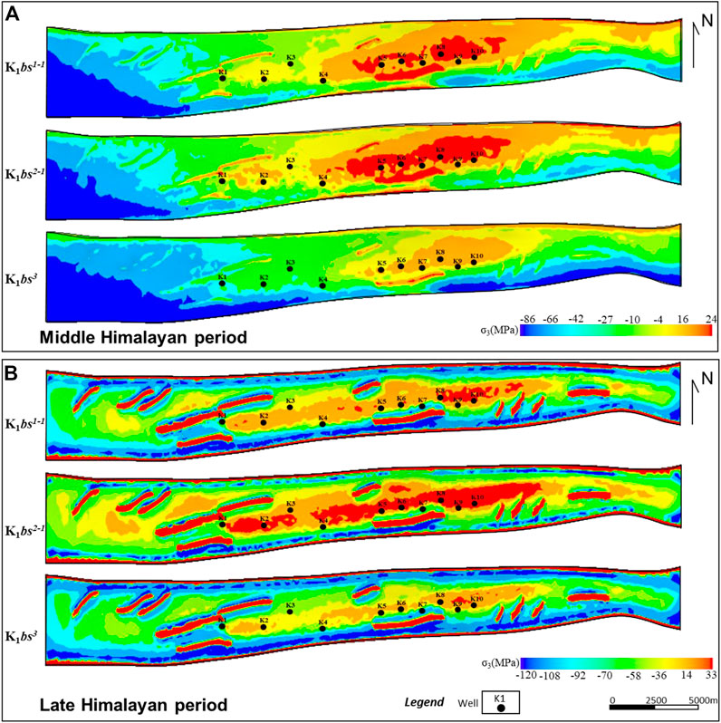
FIGURE 10. Distribution of paleo-tectonic stress field in different period. (A) Minimum principal stress in middle Himalayan period of target layer; (B) Minimum principal stress in late Himalayan period of target layer.

FIGURE 11

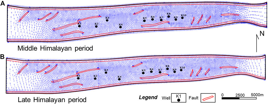
FIGURE 11. Distribution characteristics of maximum principal stress direction of tectonic stress field in different periods. (A) Direction of maximum principal stress in middle Himalayan period of target layer; (B) Direction of maximum principal stress in late Himalayan period of target layer.

5.2 Fracture distribution and its controlling factors

The spatial predictions showed that the fracture linear density (D_lf) of Keshen gas field was significantly different in the two periods of tectonic movement. As shown in Figure 12A, the well-developed fracture areas under middle Himalayan movement were primarily located on (1) the central part of Keshen anticline; (2) the structural high parts of fold core; (3) the southern major fault zone and the hanging wall of large-scale faults; and (4) along the long axis of anticline. Vertically, the D_lf of fractures at the top of the anticline was higher than 2.25 m⁻¹ in most areas of K₁bs², higher than 2.25 m⁻¹ in only some areas of K₁bs¹ and widely lower than 2.25 m⁻¹ in K₁bs³. Locally, the distribution of D_lf was still different at the top of the anticline of three lithologic members. For example, the D_lf in the east was higher than that in the west, the south was higher than the north, and the saddle between the two high points was lower. Nevertheless, the development and distribution of fractures in the middle Himalayan were mainly controlled by folding, followed by buried depth or lithofacies, and then by faulting.

FIGURE 12

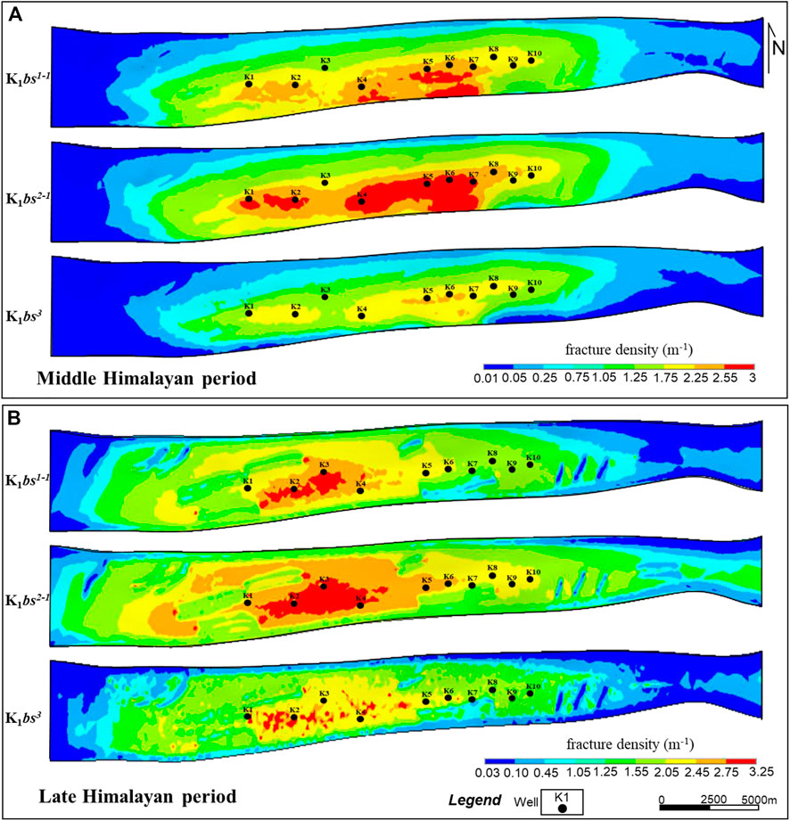
FIGURE 12. Spatial distribution of fracture development degree in different period. (A) Fracture linear density in Middle Himalayan period; (B) Fracture linear density in late Himalayan period.

Compared with the middle Himalayan, the D_lf of fractures in the late tectonic movement increased significantly, reaching more than 3.25 m⁻¹, and the high-value areas were widely distributed (Figure 12B). On the plane, the high-value areas of D_lf in this period gradually migrated to the west of anticline, and concentrated to the core of anticline. For example, in K₁bs², the D_lf near wells K1, K2, K3 and K4 of the anticline core was mostly above 3.25 m⁻¹. For example, the D_lf in the core of the anticline or near wells K1, K2, K3, and K4 was more than 3.25 m⁻¹. Interestingly, contrary to the characteristics of the middle Himalayan period, the D_lf around the secondary faults, especially the en-echelon faults, presented as low values. For this reason, combined with the tectonic evolution history and acoustic emission results, it can be concluded that most of the secondary faults of Keshen anticline formed in middle Himalayan and inherited activities in late Himalayan. In other words, these faults were where stress was easily concentrated when they were formed, controlling the development of local fractures. However, these faults were not easy to cause stress concentration as weak zones in later activities, and thus did not no longer control the generation of more fractures. As mentioned above, the development of Keshen anticline was mainly controlled by the strong thrusting of the southern major fault during the early stage, and by the combined action of the northern backward fault and southern major fault in the late stage. Under this background, the high-value areas of D_lf was mainly located near the southern major and secondary faults during the early stage, and migrated northward and westward along with the fold hinge in the late stage.

After superposition calculation of D_lf in two stages, it was found that, the well-developed fracture areas were primarily located on (1) around the fold core or along the hinge line; (2) the structural and stratigraphic high parts; and (3) shared hanging wall of two EW-striking thrust faults (Figure 13). Based on the west-east section of 3D simulation results, the total D_lf of K₁bs¹ and K₁bs² in Keshen gas field was significantly higher than that of K₁bs³, and that of K₁bs² was slightly higher than that of K₁bs¹. Among them, the total D_lf exceeded 3.15 m⁻¹ in many areas of K₁bs², while only a few areas of K₁bs³ exceeded 3 m⁻¹. As shown in Figure 13, on the whole, the distribution of the predicted total D_lf was highly consistent with the FMI interpretations of wells.

FIGURE 13

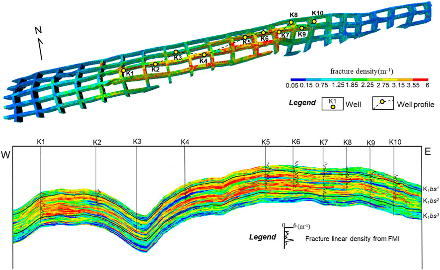
FIGURE 13. The 3D simulation results and profile distribution characteristics of fracture total density in E-W direction.

5.3 Validation of geomechanical models

As can be seen from Figure 13 and Figure 14, the overall numerical simulations in wells were in good agreement with the results of core observations and FMI interpretations. Comprehensively, the relative error of simulation results for fracture density was mostly less than 20% and the individual exceeded 30%, such as well K8 (Figure 14A). In fact, a series of soft or weak argillaceous interbeds are developed in continental tight sandstones, which have strong plastic characteristics and are difficult to produce fractures. However, due to the limitation of the grid size of geological modeling and FE software, it is difficult to take such small or thin interlayer into account, which leads to the error of numerical simulation results. Numerous production practices prove that fractures are not only the important seepage channels but also determine the high and stable yield of the tight sandstone reservoir. As shown in Figure 14B, the high-productivity wells of gas reservoir were basically consistent with the high-value areas of fracture density, except for individual wells. For example, the productivity or absolute open flow (AOF) of well K3 at the western high point of Keshen anticline reached 491×10⁴ m³/d, but its fracture density was less than 0.7 m⁻¹, and there was a mismatch. Core observation showed that the fracture dip angle of well K3 was nearly 90° and the mineral filling rate of core statistics was only 0.14. It can be inferred that the fracture effectiveness or connectivity of the target layer of this well was better, which is probably the main factor for higher productivity. All the above descriptions show that the fracture mechanics models and prediction results based on the principle of minimum energy consumption in this study are reasonable and reliable. Nevertheless, affected by the degree of geological knowledge and the limitations of modeling software, there is still a long way to go to achieve a complete, accurate and quantitative prediction of the spatial distribution of deep fractures.

FIGURE 14

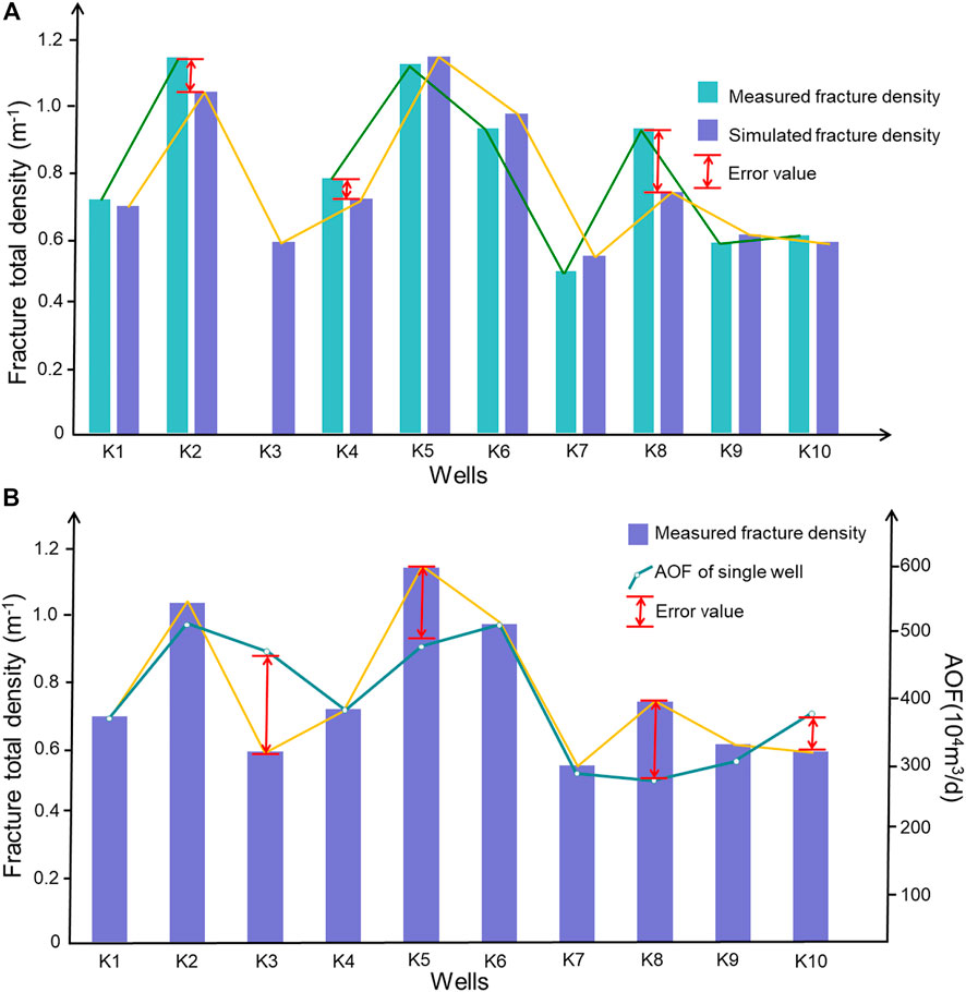
FIGURE 14. Comprehensive validation of the prediction results of 3D fracture distribution. (A) Comparison of the measured fracture density and simulated fracture density in wells of study area; (B) Relationship between gas well productivity and fracture contribution in Keshen gas field.

6 Conclusion

1) The spatial distribution of multi-stage fractures in ultra-deep Keshen gas field was clarified. The geological analysis method based on drilling core and FMI, rock mechanics experiment, and the FE numerical simulation based on principle of minimum energy consumption were adopted to carry out fracture prediction study. This novel method can help further understand the spatial distribution of fractures in complex ultra-deep tight sandstone reservoirs.

2) There were three main periods of structural fractures in the study area, and the fractures in the middle and late Himalayan periods were the most important for oil and gas migration and accumulation. The fractures in the latter two stages accounted for about 90% of the total number, most of which were unfilled and semi filled, and were important factors influencing the productivity of gas reservoirs.

3) The heterogeneity of fracture development and distribution in the Keshen gas reservoir was extremely strong. The primary factor of fracture development was folding, followed by lithofacies and buried depth, and finally thrust faulting. On the whole, the high-value areas of fracture density were mainly located at the top of fold and complicated by secondary faults and local topography, which was mainly reflected in the variation of stress field.

4) Two FE models of Keshen gas field during the middle and late Himalayan periods incorporating various lithologies, multiscale faults, mechanical parameters, constitutive model, failure criterion and fracture mechanics models was constructed to simulate the spatial fracture distributions. The overall geomechanical modeling results were in agreement with in-situ core observations, FMI analysis and AOF of wells. The novel method presented in this study is also applicable to quantitative prediction of fractures in deep reservoirs in other areas.

Data availability statement

The original contributions presented in the study are included in the article/supplementary material, further inquiries can be directed to the corresponding author.

Author contributions

JF: Conceptualization, Methodology, Writing-Reviewing and Editing, Supervision. SL: Data curation, Writing-Original draft preparation. JO: Software, Visualization, Investigation, Validation. GuL: Actual production data collection. GaL: Actual production verification.

Funding

This research was financially supported by the CNPC Major Science and Technology Project (ZD2019-183-006), the National Natural Science Foundation of China (42072234).

Acknowledgments

The authors greatly appreciate the reviewers and editors, whose opinions improved the quality manuscript.

Conflict of interest

Authors GuL and GaL were employed by the company PetroChina Dagang Oilfield.

The remaining authors declare that the research was conducted in the absence of any commercial or financial relationships that could be construed as a potential conflict of interest.

Publisher’s note

All claims expressed in this article are solely those of the authors and do not necessarily represent those of their affiliated organizations, or those of the publisher, the editors and the reviewers. Any product that may be evaluated in this article, or claim that may be made by its manufacturer, is not guaranteed or endorsed by the publisher.

References

Ass, A. S., and Mat, M. A. (2021). Finite element simulation of elastoplastic behavior of nanoporous metals using bicontinuous RVE models. Procedia Struct. Integr. 32, 230–237. doi:10.1016/j.prostr.2021.09.033

CrossRef Full Text | Google Scholar

Ay, A., Sn, A., Hk, A., Ps, A., Ap, A., and Rc, B. (2019). A case study of azimuthal fracture characterization in Cambay Basin, India. J. Appl. Geophys. 169, 239–248. doi:10.1016/j.jappgeo.2019.07.003

CrossRef Full Text | Google Scholar

Barton, N., Bandis, S., and Bakhtar, K. (1985). Strength, deformation and conductivity coupling of rock joints. Int. J. Rock Mech. Min. Sci. Geomechanics Abstr. 22, 121–140. doi:10.1016/0148-9062(85)93227-9

CrossRef Full Text | Google Scholar

Chu, G. X., Shi, S., Shao, L. Y., Wang, H. Y., and Guo, Z. H. (2014). Contrastive study on geological characteristics of cretaceous Bashijiqike Formation in Keshen2 and Kela2 gas reservoirs in kuqa depression. Geoscience 28 (3), 604–610.

Google Scholar

Conti, J., Holtberg, P., Diefenderfer, J., Larose, A., Turnure, J. T., and Westfall, L. (2016). International energy outlook 2016 with projections to 2040. United States: OSTI. doi:10.2172/1296780

CrossRef Full Text | Google Scholar

Cumella, S. P., and Scheevel, J. (2008). “The influence of stratigraphy and rock mechanics on Mesaverde gas distribution, Piceance Basin, Colorado,” in Understanding, exploring, and developing tight-gas sands. AAPG hedberg series. Editors S. P. Cumella, K. W. Shanley, and W. K. Camp, 3, 137–155.

Google Scholar

Dai, J. S., Feng, J. W., Li, M., and Wang, J. (2011). Discussion on the extension law of structural fracture in sand-mud interbed formation. Earth Sci. Front. 18 (2), 277–283.

Google Scholar

De Jarnett, B. B., Lim, F. H., Krystinik, L. F., and Bacon, M. L. (2001). Greater green river basin production improvement project (U S A: U. S. Department of Energy, Federal Energy Technology Center). Contract no. DE-AC21-95MC31063 (final report.

Google Scholar

Deng, S. G., Wang, Y., Hu, Y. Y., Ge, X. M., and He, X. Q. (2013). Integrated petrophysical log characterization for tight carbonate reservoir effectiveness: A case study from the longgang area, sichuan basin, China. Pet. Sci. 10 (3), 336–346. doi:10.1007/s12182-013-0282-5

CrossRef Full Text | Google Scholar

Ding, W. L., Wang, X. H., Hu, Q. J., Yin, S., Cao, X. Y., and Liu, J. J. (2015). Progress in tight sandstone reservoir fractures research. Adv. EARTH Sci. 30 (7), 737–750. doi:10.11867/j.issn.1001-8166.2015.07.0737

CrossRef Full Text | Google Scholar

Eberhardt, E., Stead, D., Stimpson, B., and Read, R. S. (1998). Identifying crack initiation and propagation thresholds in brittle rock. Can. Geotech. J. 35 (2), 222–233. doi:10.1139/t97-091

CrossRef Full Text | Google Scholar

Feng, J. W., Sun, J. F., Zhang, Y. J., Dai, J. S., Wei, H. H., Quan, L. S., et al. (2020). Control of fault-related folds on fracture development in kuqa depression, Tarim Basin. OIL & Gas. Geol. 41 (3), 15.

Google Scholar

Gdoutos, E. E. (2012). Crack growth instability studied by the strain energy density theory. Arch. Appl. Mech. 82 (10-11), 1361–1376. doi:10.1007/s00419-012-0690-9

CrossRef Full Text | Google Scholar

Golf-Racht, T. D. V. (1982). Fundamentals of jointed reservoir engineering. New York, NY, USA: Elsevier Scientific.

Google Scholar

Gudmundsson, A., Simmenes, T. H., Larsen, B., and Philipp, S. L. (2010). Effects of internal structure and local stresses on fracture propagation, deflection, and arrest in fault zones. J. Struct. Geol. 32, 1643–1655. doi:10.1016/j.jsg.2009.08.013

CrossRef Full Text | Google Scholar

Hennings, P. H., Olson, J. E., and Thompson, L. B. (2000). Combining outcrop data and three-dimensional structural models to characterize fractured reservoirs. AAPG Bull. 84, 830–849.

Google Scholar

Hoek, E., and Brown, E. T. (1980). Underground excavations in rock. London, UK: The Institution of Mining and Metallurgy, 80–101.

Google Scholar

Jiu, K., Ding, W. L., Huang, W. H., You, S. C., Zhang, Y. Q., and Zeng, W. T. (2013). Simulation of paleotectonic stress fields within Paleogene shale reservoirs and prediction of favorable zones for fracture development within the Zhanhua Depression, Bohai Bay Basin, east China. J. Pet. Sci. Eng. 110, 119–131. doi:10.1016/j.petrol.2013.09.002

CrossRef Full Text | Google Scholar

Ju, W., Hou, G. T., and Zhang, B. (2014). Insights into the damage zones in fault-bend folds from geomechanical models and field data. Tectonophysics 610, 182–194. doi:10.1016/j.tecto.2013.11.022

CrossRef Full Text | Google Scholar

Ju, W., Wu, C. F., Wang, K., Sun, W. F., Li, C., and Chang, X. X. (2017). Prediction of tectonic fractures in low permeability sandstone reservoirs: A case study of the Es3m reservoir in the block shishen 100 and adjacent regions, dongying depression. J. Pet. Sci. Eng. 156, 884–895. doi:10.1016/j.petrol.2017.06.068

CrossRef Full Text | Google Scholar

Kim, J. S., Lee, K. S., Cho, W. J., Choi, H. J., and Cho, G. C. (2015). A comparative evaluation of stress-strain and acoustic emission methods for quantitative damage assessments of brittle rock. Rock Mech. Rock Eng. 48, 495–508. doi:10.1007/s00603-014-0590-0

CrossRef Full Text | Google Scholar

Krajcinovic, D. (1989). Damage mechanics. Mech. Mater. 8 (2-3), 117–197. doi:10.1016/0167-6636(89)90011-2

CrossRef Full Text | Google Scholar

Kravchenko, S. G., Kravchenko, O. G., and Sun, C. T. (2014). A two-parameter fracture mechanics model for fatigue fracture growth in brittle materials: Eng. Eng. Fract. Mech. 119, 132–147. doi:10.1016/j.engfracmech.2014.02.018

CrossRef Full Text | Google Scholar

Laubach, S. E. (2003). Practical approaches to identifying sealed and open fractures. Am. Assoc. Pet. Geol. Bull. 87, 561–579. doi:10.1306/11060201106

CrossRef Full Text | Google Scholar

Leykin, V. Z. (2015). Basic laws of the processes and the principle of minimum energy consumption during pneumatic transport and distribution of pulverized fuel in direct pulverized fuel preparation systems. Therm. Eng. 62 (8), 564–571. doi:10.1134/s0040601515080042

CrossRef Full Text | Google Scholar

Li, L., Tang, H. M., Wang, Q., Tang, S. L., Feng, W., and Wang, Z. F. (2017). Diagenetic evolution of cretaceous Ultra⁃Deep reservoir in keshen belt, Kelasu thrust belt, kuqa depression. XINJIANG Pet. Geol. 38 (01), 7–14.

Google Scholar

Li, Z. J. (2011). Research on the law of fracture initiation and propagation based on principle of minimum consume energy. Daqing, China: Northeast Petroleum University.

Google Scholar

Li, Z., Luo, W., Zeng, B. Y., Liu, J. Q., and Yu, J. B. (2018). Fluid-rock interactions and reservoir formation driven by multiscale structural deformation in basin evolution. Earth Sci. 43 (10), 3498–3510. doi:10.3799/dqkx.2018.323

CrossRef Full Text | Google Scholar

Lisle, R. S. (1994). Detection of zones of abnormal strains in structures using Gaussian curvature analysis. AAPG Bull. 78, 1811–1819.

CrossRef Full Text | Google Scholar

Liu, J. S., Ding, W. L., Yang, H. M., Wang, R. Y., Yin, S., Li, A., et al. (2017). 3D geomechanical modeling and numerical simulation of in-situ stress fields in shale reservoirs: A case study of the lower cambrian niutitang Formation in the cen'gong block, south China. South China Tectonophys. 712-713, 663–683. doi:10.1016/j.tecto.2017.06.030

CrossRef Full Text | Google Scholar

Lu, H., Lu, X. S., Fan, J. J., Wang, X. H., Fu, X. F., Zhang, B., et al. (2016). Controlling effect of fractures on gas accumulation and production within the tight sandstone: A case study on the jurassic dibei gas reservoir in the eastern part of the kuqa foreland basin, China. J. Nat. Gas Geoscience 1, 61–71. doi:10.1016/j.jnggs.2016.05.003

CrossRef Full Text | Google Scholar

Luo, Y. S., Tang, S. H., Liu, C. W., and Zhou, Z. B. (2009). Advances on the least energy consumption principle and its application. Ournalofrailw. Sci. Eng. 2, 82–89.

Google Scholar

Mckinnon, S. D., and Barra, I. G. (1998). Fracture initiation, growth and effect on stress field: A numerical investigation. J. Struct. Geol. 20, 1663–1672.

CrossRef Full Text | Google Scholar

McLennan, J. A., Allwardt, P. F., Hennings, P. H., and Farrell, H. E. (2009). Multivariate fracture intensity prediction: Application to Oil Mountain anticline, Wyoming. Am. Assoc. Pet. Geol. Bull. 3 (11), 1585–1595. doi:10.1306/07220909081

CrossRef Full Text | Google Scholar

Olson, J. E., Laubach, S. E., and Lander, R. H. (2009). Natural fracture characterization in tight gas sandstones: Integrating mechanics and diagenesis. Am. Assoc. Pet. Geol. Bull. 93 (11), 1535–1549. doi:10.1306/08110909100

CrossRef Full Text | Google Scholar

Peng, Y., Li, Y. M., and Zhao, J. Z. (2016). A novel approach to simulate the stress and displacement fields induced by hydraulic fractures under arbitrarily distributed inner pressure. J. Nat. Gas Sci. Eng. 35, 1079–1087. doi:10.1016/j.jngse.2016.09.054

CrossRef Full Text | Google Scholar

Peng, Y., Zhao, J. Z., Sepehrnoori, K., and Li, Z. L. (2020). Fractional model for simulating the viscoelastic behavior of artificial fracture in shale gas. Eng. Fract. Mech. 228, 106892. doi:10.1016/j.engfracmech.2020.106892

CrossRef Full Text | Google Scholar

Peng, Y., Zhao, J. Z., Sepehrnoori, K., Li, Z. L., and Xu, F. (2019). Study of delayed creep fracture initiation and propagation based on semi-analytical fractional model. Appl. Math. Model. 72, 700–715. doi:10.1016/j.apm.2019.03.034

CrossRef Full Text | Google Scholar

Price, N. J. (1966). Fault and joint development in brittle and semi-brittle rock. Oxford, UK: Pergamon Press, 133–164.

Google Scholar

Sanz, P. F., Pollard, D. D., Allwardt, P. F., and Borja, R. I. (2008). Mechanical models of fracture reactivation and slip on bedding surfaces during folding of the asymmetric anticline at Sheep Mountain, Wyoming. J. Struct. Geol. 30, 1177–1191. doi:10.1016/j.jsg.2008.06.002

CrossRef Full Text | Google Scholar

Shanley, K. W., and Cluff, R. M. (2015). The evolution of pore-scale fluid-saturation in low-permeability sandstone reservoirs. Am. Assoc. Pet. Geol. Bull. 99, 1957–1990. doi:10.1306/03041411168

CrossRef Full Text | Google Scholar

Shrivastava, C., and Lawatia, R. (2011). “Tight gas reservoirs: Geological evaluation of the building blocks,” in SPE Middle East unconventional gas conference and exhibition, 31 january-2 february (Oman: Muscat).

CrossRef Full Text | Google Scholar

Smart, K. J., Ferrill, D. A., Morris, A. P., and McGinnis, R. N. (2012). Geomechanical modeling of stress and strain evolution during contractional fault-related folding. Tectonophysics 576 (577), 171–196. doi:10.1016/j.tecto.2012.05.024

CrossRef Full Text | Google Scholar

Solano, N., Zambrano, L., and Aguilera, R. (2011). Cumulative-gas-production distribution on the nikanassin tight gas formation, alberta and British columbia, Canada. SPE Reserv. Eval. Eng. 14, 357–376. doi:10.2118/132923-PA

CrossRef Full Text | Google Scholar

Song, H. Z. (1999). An attempt of quantitative prediction of natural fracture on brittle rock reservoir. J. Geomech. 5, 76–84.

Google Scholar

Song, Z. Z., Liu, G. D., Yang, W. W., Zhou, H., Sun, M., and Wang, X. (2017). Multi-fractal distribution analysis for pore structure characterization of tight sandstone-A case study of the Upper Paleozoic tight formations in the Longdong District, Ordos Basin. Mar. Petroleum Geol. 92, 842–854. doi:10.1016/j.marpetgeo.2017.12.018

CrossRef Full Text | Google Scholar

Sun, M. C., Xu, W. Y., Wang, S. S., Wang, R. B., and Wang, W. (2018). Study on damage constitutive model of rock based on principle of minimum dissipative energy. J. Central South Univ. Sci. Technol. 49 (08), 2067–2075.

Google Scholar

Sun, S., Hou, G. T., and Zheng, C. F. (2017). Fracture zones constrained by neutral surfaces in a fault-related fold: Insights from the Kelasu tectonic zone, Kuqa Depression. J. Struct. Geol. 104, 112–124. doi:10.1016/j.jsg.2017.10.005

CrossRef Full Text | Google Scholar

Tabarrok, B., and Leech, C. M. (2002). Hamiltonian mechanics for functionals involving second-order derivatives. J. Appl. Mech. 69 (6), 749–754. doi:10.1115/1.1505626

CrossRef Full Text | Google Scholar

Tan, C. X., and Wang, L. J. (1999). An approach to the application of 3_D tectonic stress field numerical simulation in structural fissure analysis of the oil-gas-bearing basin. Acta Geosci. Sin. 20, 392–394.

Google Scholar

Taylor, T. R., Giles, M. R., Hathon, L. A., Diggs, T. A., Braunsdorf, N. R., Birbiglia, G. V., et al. (2010). Sandstone diagenesis and reservoir quality prediction: Models, myths, and reality. Am. Assoc. Pet. Geol. Bull. 94 (8), 1093–1132. doi:10.1306/04211009123

CrossRef Full Text | Google Scholar

Tojaga, V., Kulachenko, A., Stlund, S., and Gasser, T. C. (2021). Modeling multi-fracturing fibers in fiber networks using elastoplastic timoshenko beam finite elements with embedded strong discontinuities-formulation and staggered algorithm. Comput. Methods Appl. Mech. Eng. 384, 113964. doi:10.1016/j.cma.2021.113964

CrossRef Full Text | Google Scholar

Tuckwell, G. W., Lonergan, L., and Jolly, R. J. H. (2003). The control of stress history and flaw distribution on the evolution of polygonal fracture networks. J. Struct. Geol. 25, 1241–1250. doi:10.1016/s0191-8141(02)00165-7

CrossRef Full Text | Google Scholar

Wlderhaug, O., Eliassen, A., and Aase, N. E. (2012). Prediction of permeability in quartz-rich sandstones: Examples from the Norwegian continental shelf and the Fontainebleau sandstone. J. Sediment. Res. 82 (12), 899–912. doi:10.2110/jsr.2012.79

CrossRef Full Text | Google Scholar

Wang, R., Ding, W., Zhang, Y., Wang, Z., Wang, X., He, J., et al. (2016). Analysis of developmental characteristics and dominant factors of fractures in lower cambrian marine shale reservoirs: A case study of niutitang Formation in cen’gong block, southern China. J. Pet. Sci. Eng. 138, 31–49. doi:10.1016/j.petrol.2015.12.004

CrossRef Full Text | Google Scholar

Wu, Z. H., Zuo, Y. J., Wang, S. Y., Chen, J., Wang, A. L., Liu, L. L., et al. (2017). Numerical study of multi-period palaeotectonic stress fields in lower cambrian shale reservoirs and the prediction of fractures distribution: A case study of the niutitang formation in feng'gang No. 3 block, south China. Mar. Petroleum Geol. 80, 369–381. doi:10.1016/j.marpetgeo.2016.12.008

CrossRef Full Text | Google Scholar

Xue, Y. C., Cheng, L. S., Mou, J. Y., and Zhao, W. (2014). A new fracture prediction method by combining genetic algorithm with neural network in low-permeability reservoirs. J. Petroleum Sci. Eng. 121, 159–166. doi:10.1016/j.petrol.2014.06.033

CrossRef Full Text | Google Scholar

Zeng, L. B., and Li, Y. G. (2010a). Tectonic fractures in tight gas sandstones of the upper triassic xujiahe formation in the western sichuan basin, China. Acta Geol. Sin. - Engl. Ed. 84 (5), 1229–1238. doi:10.1111/j.1755-6724.2010.00293.x

CrossRef Full Text | Google Scholar

Zeng, L. B., Wang, H. J., Gong, L., and Liu, B. M. (2010b). Impacts of the tectonic stress field on natural gas migration and accumulation: A case study of the kuqa depression in the Tarim Basin, China. Mar. Pet. Geol. 27, 1616–1627. doi:10.1016/j.marpetgeo.2010.04.010

CrossRef Full Text | Google Scholar

Zeng, Q. L., Zhang, R. H., and Lu, W. Z. (2017). Fracture development characteristics and controlling factors based on 3D laser scanning technology: An outcrop case study of Suohan village, Kuqa foreland area. Tarim. Basin Nat. Gas. Geosci. 28 (3), 397–409.

Google Scholar

Zhang, Y. Z., Feng, J. W., Luo, R. L., and Liu, Z. L. (2020). Study of controlling factors on productivity of keshen gas field: A deep tight sandstone reservoir in kuqa depression. IOP Conf. Ser. Earth Environ. Sci. 555 (1), 012107. (5pp). doi:10.1088/1755-1315/555/1/012107

CrossRef Full Text | Google Scholar

Zhang, Z. P., Wang, Q. C., and Wang, Y. (2006). Brittle structure sequence in the Kuqa Depression and its implications to the tectonic paleostress. Earth Science-Journal China Univ. Geosciences 31 (3), 310–316.

Google Scholar

Zhao, G. J., Li, X. Q., Liu, M. C., Dong, C. Y., Li, J., Liu, Y., et al. (2022). Fault activity and hydrocarbon accumulation significance of structural belt in northern Kuqa Depression. J. Min. Sci. Technol. 7 (01), 34–44. doi:10.19606/j.cnki.jmst.2022.01.004

CrossRef Full Text | Google Scholar

Zhao, W. T., Hou, G. T., and Sun, X. W. (2013). Influence of layer thickness and lithology on the fracture growth of clastic rock in East Kuqa. Geotect. Metallogenia 37 (4), 603–610.

Google Scholar

Zhou, G. X., Ye, Y., and Zhou, F. J. (2021). Research progress in damage assessment methods for tight sandstone gas reservoirs. J. Phys. Conf. Ser. 1, 12033. doi:10.1088/1742-6596/2009/1/012033

CrossRef Full Text | Google Scholar

Zhou, X. G., Cao, C. J., and Yuan, J. Y. (2003). The status and prospects of quantitative structural joint prediction of reservoirs and research of oil and gas seepage law. Adv. Earth Sci. 18, 398–404.

Google Scholar