 Nelly Moulin
 Frederic Gresselin
 Bruno Dardaillon3
 Zahra Thomas
- 1Intitut Agro, UMR 1069 SAS, Rennes, France
- 2DREAL Normandie, Caen, France
- 3Université de Caen-Normandie, LMNO, UMR 6139, Rennes, France
In the context of global warming, river management is essential to maintain favourable water temperature ranges for aquatic species. Therefore, understanding the main factors influencing the water temperature becomes a key part in the management process. In this paper, we used Independent Component Analysis (ICA) to identify these main factors and improve water temperature forecasting. The study is caried out on two rivers in Normandy (France) with quite different characteristics. Each river was equipped with several temperature sensors which series range from 2011 to 2021. The ICA analysis of the data series reveals that the thermal regime of these two rivers is mainly controlled by seasonal and daily climatic factors. The Sélune regime also turns out to be influenced by the presence of a dam, dismantled during the monitoring of the river. The temperature of the Odon appears to be clearly controlled by seasonal lightening conditions in connection with the presence of the riparian vegetation. Complementary, an innovative approach called “successive ICA” is used to reconstruct the natural thermal regime of the Sélune without the presence of the dam. Emphasis is therefore placed here on the interest of ICA in hydrology as en elementary method for extracting the main influencing factors and quantifying their importance on the thermal regime of a river. It also allows to remove the influence of a particular factor and reconstruct time series better suited for temperature forecasting. The method used here is not specific to temperature time series and can be applied to any region even with different hydrological characteristics.
1 Introduction
Temperature is a key parameter in river ecology as it influences the environment and several species life cycles (Magnuson et al., 1979; Ebersole et al., 2001; Daufresne and Boët, 2007; Caissie, 2006; Comte et al., 2013; Souchon and Tissot, 2012). Thermal regimes are mainly influenced by atmospheric factors at the site scale, at the catchment scale or at larger ones (Webb and Walling, 1993; Poole and Berman, 2001; Webb et al., 2008; Ryan et al., 2013; Hannah and Garner, 2015; Jones and Schmidt, 2018). Atmosphere-water heat transfers, and to a lesser extent water-aquifer transfers, control the major part of thermal variation in large rivers (Sinokrot and Stefan, 1994; Evans et al., 1998; Lalot et al., 2015). These transfers vary with the residence time of the water in the environment and the river’s width. Also, water temperature increases from upriver to downriver, with a mean gradient of 0.1°C/km for large plain rivers (Torgersen et al., 2001), until reaching an equilibrium temperature. Thermal regimes are also influenced by the river flow, the geo-morphology, the riparian vegetation or hydraulic constructions (Kelleher et al., 2012; Arismendi et al., 2013; Ryan et al., 2013; Johnson et al., 2013; Jackson et al., 2017; Garner et al., 2017; Dugdale et al., 2018; Beaufort et al., 2020).
In France, most big rivers are monitored in temperature since the 70 s or 80 s (in accordance with the electricity production) (Moatar and Gailhard, 2006; Poirel et al., 2008; Larnier et al., 2010). Environmental monitoring developed from 2008 thanks to a national network created by the French Office for Biodiversity in order to better understand river ecology. In Normandy, the Regional Directorate for Planning and Housing (DREAL) equipped about one-third of the 18.000 km Normand rivers.
A particular focus is held on dams’ effects. Dams and reservoirs usually have a significant impact on rivers temperature (Webb and Walling, 1993; Poirel et al., 2010; Seyedhashemi et al., 2021). Large dams tend to decrease rivers temperature in summer and to modify annual cycles whereas ponds and shallow reservoirs (less than 15 m) tend to increase the temperature (Seyedhashemi et al., 2021). This is because the solar radiation heats the surface layers faster than deeper layers. Even smaller dams (water drops less than 2 m) can strongly influence rivers’ thermal regime by increasing the temperature (Chandesris et al., 2019). Dams’ impact depends on the surface, the depth and the residency time in the structure. Thus, rivers with dams present a different thermal signature than natural rivers. In the Loire catchment (North-West of France), dam-equipped rivers can have a mean temperature higher than the air temperature (Ta) all year long (Seyedhashemi et al., 2021).
In this paper, the thermal regime of two rivers in Normandy were analysed: the Sélune, influenced by 2 dams and the Odon, considered as natural. Each river was equipped with three temperature sensors to analyse the temperature along the river and identify the main influencing factors and quantify their importance on a river’s thermal regime (Table 1). Data was analysed using Independent Component Analysis (ICA), a statistical method not often used in hydrology but already tested on two other rivers in Normandy (Gresselin et al., 2021) and in several studies across the world (Hannachi et al., 2009; Aires et al., 2000; Moradkhani and Meier, 2010; Westra et al., 2008; Middleton et al., 2015; Gong et al., 2014). In addition, a new way of using ICA is proposed in order to remove some components from a signal and improve the results of a linear regression prediction model.

TABLE 1. Characteristics for each monitored location (in C). Orientation N-E-S-W stand respectively for North-East-South-West.
2 Studied catchments
2.1 The Odon catchment
The Odon catchment area extends over 217 km2. The river travels 49 km before ending in the Orne in Caen (Figure 1). The Odon flows on the Armorican massif for the most part and the Parisian massif close to the confluence with the Orne. It drains successive hills mainly composed of schist and sandstone. Three temperature sensors are installed on this river.
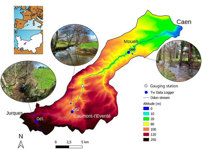
FIGURE 1. Odon catchment Digital Elevation Model (DEM) showing the water temperature (Tw) sensors’ locations from upriver to downriver: Od1, Od2 and Od3. The empty blue circle indicates the location of the gauging station providing the discharge time series. Pictures were taken in a leafless period (April 2022).
The Odon starts in a Variscan syncline where bar sandstones form high points in the Normandy region. The river then flows along a narrow valley in a SE/NW orientation. In Od1, the corridor is around 40 m with a main channel around 1.5 m and quite shallow. The rivers flows between sills and pools in a sinuous way. Riverbanks are densely vegetated. The watertable is relatively low, varying from a few centimeters to a few decimeters at the end of winter. The riverbed is mainly composed of rough sediments. After the Variscan syncline, the Odon follows a meander from West to East then continues along a N/S orientation in Brioverian lands (hills and open valleys made of shale and sandstone).
In Od2, the corridor is 100 m wide and the main channel is an artificial 2.5 m wide section bordered with high trees. The river flows between pools and high waters with a mix of mud and stone riverbed. The watertable varies quickly up to several decimetres. Finally, near the city of Caen, the Odon drops in a chalk plateau at the west of the Parisian basin. The river takes a SW/NE orientation until its confluence with the Orne. Slopes are gentle except at the bottom of the valley where they can reach 30% (Supplementary Figure S1).
In Od3, the site is shaded from the direct influence of the Sun (especially in winter). The south side is densely forested with conifers which limits the sunlight all year long. However, the main river channel reaches 5 m wide so the middle of the river is exposed to direct sunlight in summer.
2.2 The Sélune catchment
The Sélune is one of the three coastal rivers ending in the Mont-St-Michel bay in the North-West of France (Figure 2). The catchment area is close to 1100 km2. It drains several hills on the schist-sandstone and granite Armorican massif. The Sélune travels around 76 km in total along its longitudinal profile. In the first half of the XXst century, two hydroelectric dams were built at a few kilometers from the mouth of the river: the Vezins dam and la Roche-Qui-Boit dam, respectively 36 and 16 m high. To reestablish a natural flow regime and provide ecological benefits, the French government decided to remove some facilities which did not allow certain fish species, such as European eels, to cross them. The Vezins dam was removed in 2019 and the destruction of la Roche-Qui-Boit dam is scheduled for 2022.
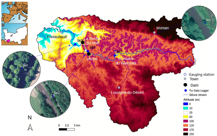
FIGURE 2. Sélune catchment DEM showing the temperature sensors’ locations. The empty blue circle indicates the location of the gauging station providing the discharge time series. Pictures were taken from the IGN database.
The river water temperature monitoring was performed using three temperature sensors installed along the river and respectively named: Se1, Se2 and Se3. Se1 is located upriver the Vezins dam and its lake (Figure 2). At this location, the river is an open site (Supplementary Figure S2), about 20 m wide and strongly influenced by atmospheric factors. Se2 is located about a hundred meters downriver the dam. At this place, the vegetation is denser and the riverbed is 19 m wide (before the dam’s removal). Se3 is located a few kilometers below la Roche-Qui-Boit dam. At this location, the river is 22 m wide and densely vegetated on the banks.
3 Times series collection and pre-processing
3.1 Temperature data
The Sélune and the Odon were equipped by the DREAL of Normandy with temperature sensors HOBO water Temp Pro v2 (U22-001) with an accuracy of ±0.2°C. The sensors were fixed on riparian trees’ roots, mostly in shaded areas and at depths which ensure a continuous immersion (except for Se2). Temperature is measured every 2 h, interpolated to a hourly basis in order to get a homogeneous time frame with other measurements (Ta, streamflow etc). In this study, for each river, a dataset of 10 years was analysed. A common time series was chosen between the 27 May 2011 and the 7 June 2021 (Table 1). Each dataset is composed of 89,490 time steps.
The temperature on both rivers evolves according to a seasonal cycle (Figure 3). Colder in winter (November to February) and warmer in summer (June to September). Minimal temperatures get close to 0°C for the Odon and the Sélune upriver and around 3°C for the Sélune downriver. The mean temperature of both rivers tends to increase downriver. This rise reaches 1°C in the Odon and 0.7°C in the Sélune. Measured maxima are higher for the Sélune which is a wider river and less shaded than the Odon. Stations on the Sélune are further from the source than stations on the Odon. The distance has an impact on the sensibility of the thermal regime to climatic factors (Le Lay et al., 2019).
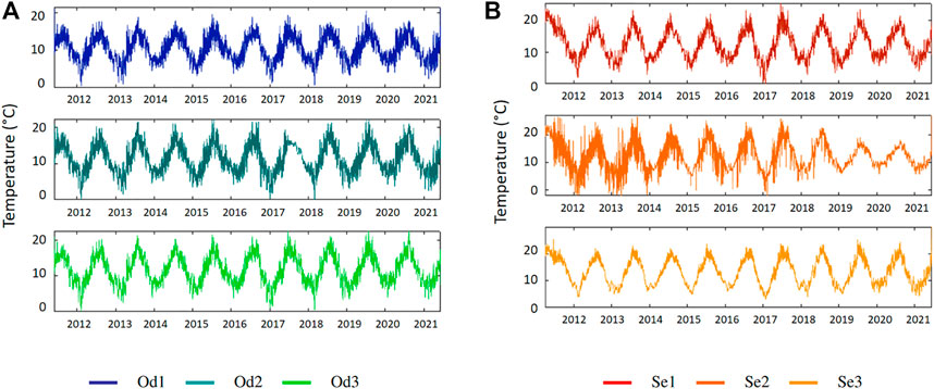
FIGURE 3. Stream temperature time series at the three location on (A) the Odon in Od1-Od2-Od3 and (B) the Sélune in Se1-Se2-Se3. Upriver stations at the top and downriver stations at the bottom.
Concerning Se2, as the temperature sensor was located at the foot of the Vezins dam, it was regularly emerged during reservoir fillings to produce electricity. Therefore, the temperature at this station could reach thermal minima way below 0°C when it was emerged because then, it measured the air temperature. After the destruction of the dam in 2019, Se2 was covered by a thick sediment layer and its thermal amplitude was reduced (Figure 3).
3.2 Pre-processing
Due to occasional sensor failures and/or maintenance operations, river temperature time series are not perfectly continuous. In total, less than 0.2% of the time steps was filtered as outliers or filled with the methods described below.
Missing data: it can affect a very specific period (a few hours only) due to maintenance operation or longer periods (several days, weeks or months) due to sensor failure. To address this defect, several strategies were considered. If the number of missing points remained low enough (less than 20 h), linear interpolation was used to fill the gap without compromising the physical evolution of the series. If more points were missing, three options were chosen depending on the needs: 1) averaging over upriver and downriver stations (if possible and if coherent); 2) simply removing this part of data from all series to perform ICA or 3) replace with the mean value of the series (in order to avoid missed raw data presented as NaN; acronym for Not a Number).
Outliers: some points displayed extreme values which were not consistent with the physics involved (such as negative water temperatures for immersed sensors). In this case, a common method was to remove data points which were further than x times the series mean value.
Homogeneous frequency: all the stations had different time depth and not all of them use the same measurement settings. This created heterogeneous time series that were difficult to compare and much less to use in ICA. To use the data, stations with a wide common time range were chosen (i.e. from the 27th May 2011 to the 7th June 2021). Also, the data frequency was set to a hourly basis. It is to be noted that the lowest measuring frequency was one point/2 h, so a temporal down scaling from 2 to 1 h did not affect the interpretation of the data.
In the following sections, all data presented were pre-processed with the methods mentioned above for the period 2011–2021.
4 The analysis methods
4.1 Independant component analysis method
ICA can identify hidden factors which influence the observed data without knowing mixing mechanisms. It can decompose one or several random non Gaussian signals X ∈ Rm in a linear combination of independent signals such as:
with
Decomposing observations in several independent sources can estimate A and S with two main hypothesis. On the one hand, the sources are statistically independent. On the other hand, not more than one independent component can have a Gaussian distribution.
Each independent component S is represented by a graph and a weight matrix A. The graph shows the variation of S with time whereas the matrix shows the variation of S with the stations.
ICA analysis was performed using the Fast-ICA package from the R software (Hyvärinen and Oja, 2000; Marchini et al., 2021). This algorithm is suited to estimate the mixing matrix A and the source matrix S. Data are centered so the initial observations X can be obtained by adding A ⋅ S to the mean of the X series.
with
4.2 The successive ICA method
In order to overcome the limit of the available datasets, we applied a successive ICA method to extract more information. This method uses the following steps.
1) From initial temperature datasets, run an ICA.
2) Sort the ICA source components and remove some of them according to the criteria listed below.
3) Build new temperature datasets by applying the corresponding matrix coefficients on the remaining components and by adding the mean value of the datasets used in 1.
4) Repeat steps 1 to 3.
This successive ICA method allows to extract further information from the first ICA components. By removing an obvious contribution after the first ICA, one can get to more complex phenomena. Choosing which ICA component to remove relies on several criteria.
• When a physical signal is clearly identified (for example a seasonal variation correlated with the air temperature).
• To isolate a specific component and identify several factors included in this specific component.
• When a signal is specific to one location and reflects a particular condition.
• When a signal is identified as a noise or as a residual signal (amplitude less than the measurement’s accuracy).
In all cases, the new dataset’s distribution should be non-Gaussian. Ultimately, the decomposition process ends when the remaining ICA components are reduced to white noise or when there is only one exploitable signal left. Therefore, after each ICA, Box-Pierce tests were performed to remove useless white noise signals in the process. In this study, signals were considered exploitable when their amplitude was larger than the sensor’s accuracy (±0.2°C). Signals with smaller amplitudes were either considered as residual signals or identified as white noise with Box-Pierce tests.
The example below shows how after extracting ICA components, a non-Gaussian component can be refined by subtracting noise signals. The main calculation steps are described below.
1) Run a first ICA with the measured time series. Identify a component to work on (here the seasonal component).
2) Recompose time series using only the chosen component multiplied by the matrix coefficient for each station and adding the measured time series mean value.
3) Run a second ICA with the three new times series.
4) Identify the seasonal component and run a Box-Pierce noise test on the two residual components.
The Box-Pierce test indicates if a signal is characteristic of a white noise with a p-value
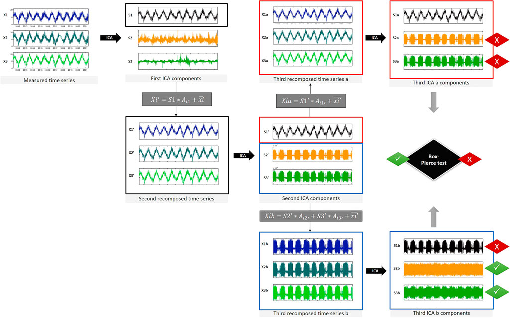
FIGURE 4. Schematic view of the successive ICA process applied on a time series.
The diagram below (Figure 4) shows the process of the successive ICA method applied to a measured time series. All ICA components in this figure were multiplied by the mean of their matrix coefficients on the three stations. From the first ICA, only the component X1 is kept (black frame). The second time series (black frame middle left) are composed from X1 only. The second ICA (red and blue frames middle) displays a seasonal component (X1’) and two other signals with very low amplitudes (
In the end, the last seasonal component X1a can be considered “cleaner” as its predecessors X1 and X1’. In this case, the residual signals show very low amplitudes so the differences between the different stages of the seasonal components remains subtle.
4.3 The successive ICA method in water temperature prediction
This study takes advantage of the successive ICA method to generate a hypothetical temperature time series on the Sélune. This new signal is a proposition of what the temperature time series in Se2 would have been if the Vezins dam had not been constructed. On a long time scale, the dam operation can be considered as temporary. For example, when confronting the river thermal regime with climate change, it could be useful to remove the effect of the dam. To do this, the following steps were applied.
1) Run a first ICA with the original temperature time series. Identify the dam component.
2) Recompose temperature time series with only the two other components (seasonal and daily) by multiplying the ICA component with the correspond matrix coefficients for each station and adding the mean value of the original time series.
3) For further information, run a second ICA with the new time series.
The chart below (Figure 5) shows in 1) the new time series on the three stations (solid black) compared with the original time series. We see that for stations Se1 and Se3, there is almost no difference as they are little affected by the dam component. The new signal is shifted by −2 °C in average. However, in Se2, we can see that the signal is more regular in the new time series. Irregular peaks and variations originating from the dam have disappeared. After 2019 and the dam’s removal, the two signals are closer and there is less difference between them.
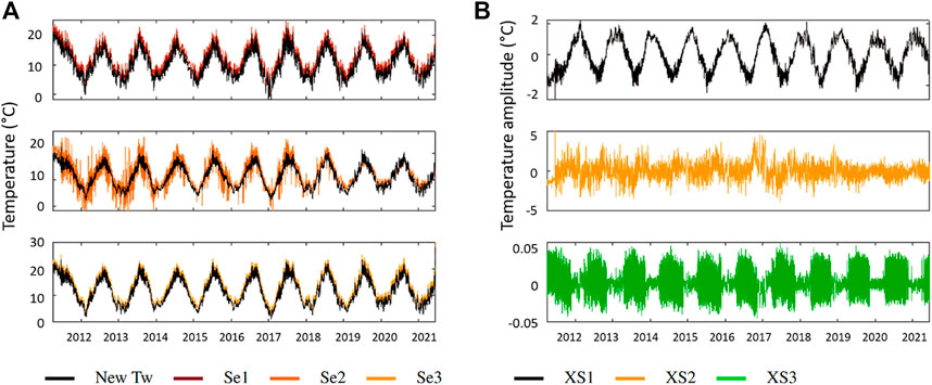
FIGURE 5. (A) Recomposed temperature time series without the dam’s ICA component in black superimposed on the measured temperature time series. (B) Second ICA with the new temperature time series from (A).
In (b), the chart shows the ICA components obtained with the new temperature datasets (black curves in Figure 5). We can recognise the seasonal component (XS1 in black) as well as the daily component (XS2 in orange). The third one (XS3 in green) is negative to the Box-Pierce noise test but shows an amplitude under the accuracy of the measuring sensor. Therefore, it is likely coming from the sensor itself and considered as a residual signal.
The interest of the successive method was tested in water temperature prediction using a regression linear model. In this test, two runs were made. First, the model was applied on original TW time series with a separation of 70–30% between the train and test data. Then, the model was applied on corrected data for the train part, which means without the dam component. The test data was kept identical to the first test. Among the three stations, the difference between the two runs was most visible on station Se2 where the dam component is the most important. Removing the dam component from the time series improved the fit between predicted and measured test data by 34.4% and contributed to reduce the RMSE by 8.9% (Table 2).
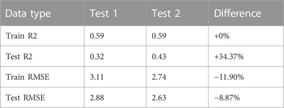
TABLE 2. Improvement in water temperature prediction on Se2 by removing the dam component.
Although this test used a simple regression model, it shows the interest of removing a particular signal which affects a temporary period. In this case, the dam itself is not supposed to affect the river thermal regime several years after its removal. By using the successive ICA method, it is easier to choose the influence of environmental factors for future thermal regimes.
5 Results and discussions
5.1 About the mixing matrix
From the temperature time series, at least three components were extracted for each river to take advantage of the number of stations in the range 2011–2021. Corresponding ICA components will herein be referred with their code names in the tables below (Table 3). For each ICA component, the mixing coefficients make the link with each station. Signs indicate the relative relationships between the components and the station. For example, XOdA shows the same kind of relationship for all stations as all the coefficients have the same sign. Then, the absolute value of the coefficients shows the impact of each component on the different stations. A high absolute value indicates a strong influence of this component on the thermal regime of the station. On the contrary, a value close to 0 means that the component has little effect on the thermal regime at this station. For example, XOdC has a strong influence in Od2 whereas it has a negligible effect in Od3.
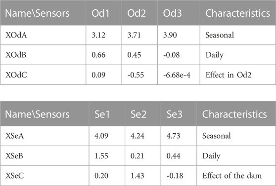
TABLE 3. Mixing matrix coefficients for the ICA components for 1) the Odon and 2) the Sélune.
From the matrix coefficients, we can see that the first components (XOdA for the Odon and XSeA for the Sélune) clearly have a dominant effect on the thermal regimes and affect all stations quite equally. On the contrary, looking at the coefficients values, XOdC affects mainly Od2 and XOdB seems correlated to the upriver stations Od1 and Od2. On the Sélune, XSeB affects the upriver station Se1 more and XSeC is clearly correlated to Se2.
At this stage, we can separate the first components which are regular and affect all stations with the same magnitude (including an increasing effect downriver) on the one hand, and other components which affect some stations in particular on the other hand. Complementary to the mixing coefficients, graphic representations of the ICA components (Figure 6) show their impacts on the stations. The graphs represent the time variation of each ICA component for each station weighted with the corresponding matrix coefficient.5b
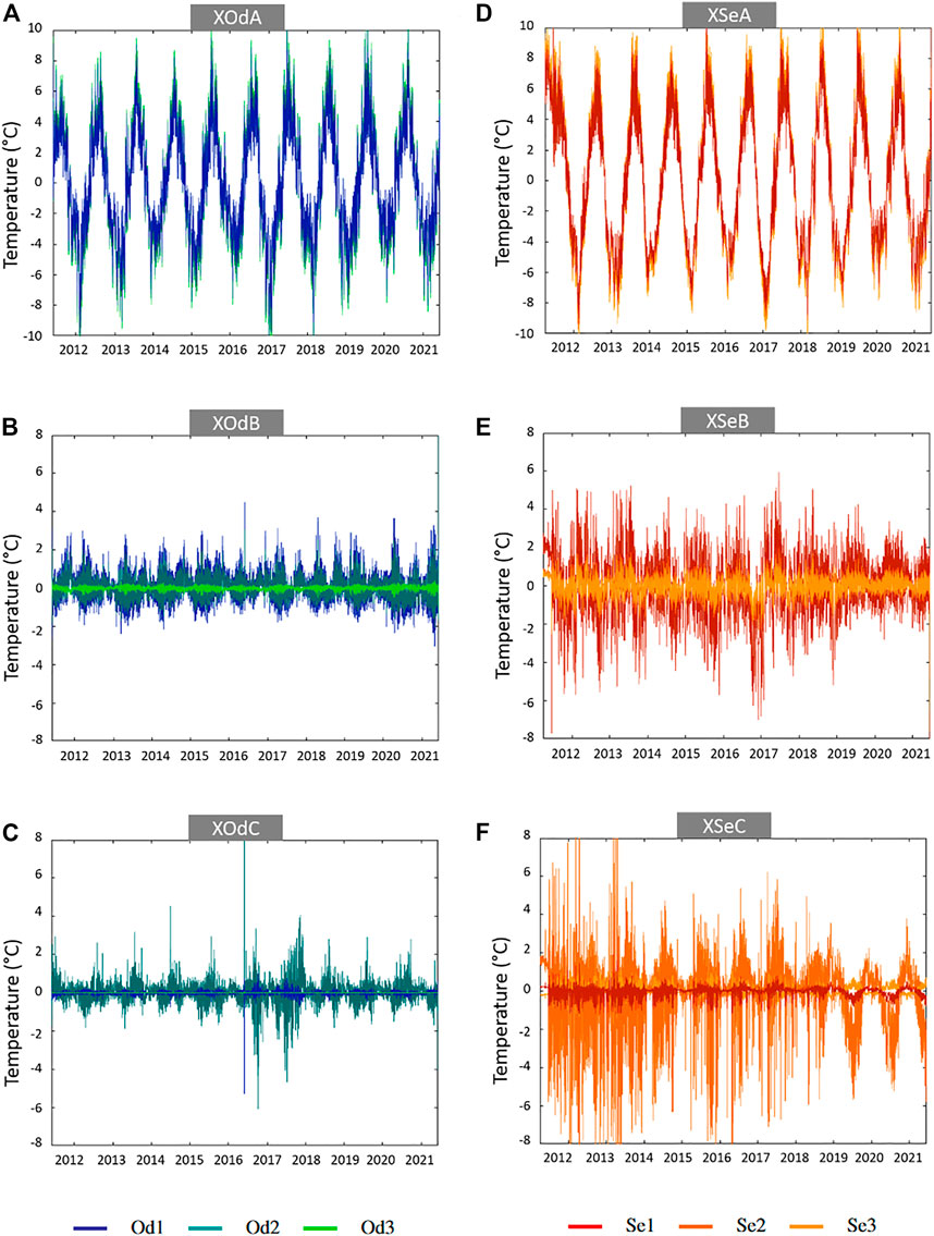
FIGURE 6. Temperature ICA components for the Odon in (A–C) and the Sélune in (D–F). (A–D) Seasonal components. (B–E) Daily components. (C) Component specific to Od1 and Od2. (F) Component linked to the Vezins dam.
On the Odon, the maximum amplitude is obtained with the first component XOdA (±10 °C). XOdB and XOdC represent secondary components of the signal with smaller amplitudes than XOdA (±2°C). Finally, Od3 displays a behaviour quite different from Od1 and Od2 based on the three ICA components. In Od3, XOdA’s matrix coefficient is the strongest of all stations whereas XOdC is almost nil and XOdB takes an opposite sign compared to Od1 and Od2.
On the Sélune however, the three components take high amplitudes depending on the stations. The maximum amplitude is observed for XSeA for all stations. Then, XSeB shows a signal half the amplitude of XSeA for station Se1 and XSeC shows an amplitude almost as high as XSeA in the period 2011–2013 for station Se3.
In the following subsections, physical factors are attributed to the different components. As the number of ICA components is limited to 3, all components can contain several factors’ signatures. Therefore, the physical factor attributed to the ICA component will concern the most visible ones. Physical factors can be separated between climatic factors at the catchment or regional scale and environmental factor at the measuring site scale.
5.2 Climatic factors
5.2.1 Seasonal variations
On both rivers, the first ICA components to come out, XOdA and XSeA, show a clear seasonal variation (Figures 6A,D). These signals have their maxima in summer and minima in winter. Due to heat reservoirs (sea and soils), maxima are shifted by half a month from the winter and summer solstices. These variations are quite similar every year. The seasonal components show the strongest matrix coefficients (Supplementary Table S3) and increase downriver for both rivers as the water-atmosphere heat exchanges increase with the surface, the distance from the source and the width of the river. On the Odon, for example, XOdA accounts for 80.6% of the three contributions in Od1 whereas it accounts for 98% in Od3. This confirms that the seasonal variation is the main physical phenomenon governing water temperature in Normandy (Gresselin et al., 2021) and in general (Caissie, 2006). Comparing the rivers, the seasonal component is stronger for the Sélune (coefficients around 4) than for the Odon (coefficients around 3). The amplitude difference can be explained by geometric factors. The Odon is a narrower river than the Sélune on the measuring sites, and thus less influenced by atmospheric factors. Also, measuring sites on the Sélune are further downriver than the ones on the Odon. Correlation factors between the seasonal components and the air temperature (Ta) rise up to 81,89% for XOdA and 76.65% for XSeA (whole time range).
The high frequency signal superimposed on the seasonal signal is mostly due to strong thermal variations caused by cyclonic and anticyclonic events (frequent in Normandy). This secondary source generates an extra signal common to all stations. On the Sélune, we can notice that the ICA component XSeA is much smoother, before 2017, than the corresponding component on the Odon. The ICA extraction attributes the high frequency variations to other factors before 2019 than a regular variation. After 2019 and the dam’s removal, the Sélune seasonal variation seems closer to a “natural” river such as the Odon and the high frequency signal appears more clearly in XSeA.
This first components XOdA and XSeA are seasonal variations strongly correlated with the air temperature. These seasonal components are not necessarily exclusive to the air temperature effect but can gather several atmospheric factors with similar behaviours.
5.2.2 Daily variations (XOdB, XSeB)
After the seasonal variations, the most important factors are daily variations (Figures 6B,E). Daily variations record day/night temperature differences over the year but without the seasonal variation. That is why XOdB and XSeB do not exhibit a “saw-tooth” type signal as for XOdA and XSeA. The ICA components XOdB and XSeB show smaller amplitudes over the year than the seasonal components XOdA and XSeA. Amplitudes vary around ±3 °C for the Odon and ±4 °C for the Sélune.
In order to highlight the different influences over the stations, typical years were selected in temperature time series for the Sélune (Figure 7) and the Odon (Figure 8). Figure 7 shows the component XSeB in 2 years: before the dam’s removal (2014) and after (2020). Figure 8 shows the component XOdB for the Odon on a typical year (2013).
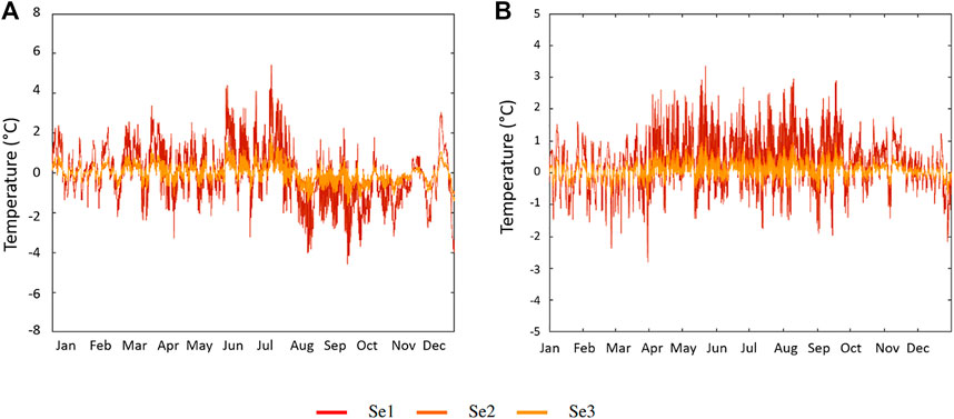
FIGURE 7. Temperature ICA component XSeB for the Sélune on typical years (A) before the dam’s removal (2014) and (B) after the dam’s removal (2020).
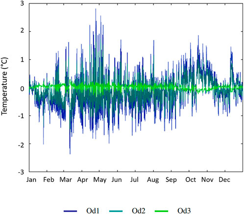
FIGURE 8. ICA component XOdB for each Odon station in 2013.
On the Sélune, XSeB is more steady throughout the year. However, we can distinguish two phases before and after the dam’s removal (Figures 7A,B). The amplitude of the variations is more important before 2019 (±5°C) than after (±2 C). Before 2019, XSeB is marked by a temperature drop in August and irregular fluctuations especially in Se1. These fluctuations remain important until mid-December where the mean temperature increases again. For this period (2011–2019), it is difficult to consider a “typical” year as the variations in XSeB are quite irregular and strong. But in average, the strongest variations occur in early summer before a drop in early autumn. XSeB in Se2 and Se3 appear steadier and vary less throughout the year whereas in Se1, it varies above and under the signal of the downriver stations. This effect in a river equipped with a dam was also observed in the Loire basin (France) (Seyedhashemi et al., 2021). After 2019, the daily variations are lower over the year and display seasonal variations as on the Odon. We can notice a higher day/night amplitude from April to October but in a relatively small range (±2°C).
On the Odon, XOdB can be described by the amplitude of the day/night variations (Figure 8). Thus, from March, the day/night amplitude increases until its maximum in May. After that, the amplitude decreases and stabilises throughout the summer. It starts to increase again in September and decreases in November to stabilise in winter. This behaviour does not follow the seasonal variation seen in XOdA but is caused by a combination of climatic factors: length of the day, day/night thermal variations as well as environmental factors described later. This component affects mainly Od1 and Od2 because the thermal variations in Od3 are almost exclusively explained by the seasonal component XOdA. As it will be described later, daily variations in Od1 and Od2 reflect a group of factors repeatable every year.
The second components XOdB and XSeB express daily variations. It contains a seasonal cycle for the Odon stations and a strong contrast before and after 2019 for the Sélune stations. Contrary to the first component it shows very different aspects on the two rivers and on the two different periods for the Sélune. Unlike XOdA and XSeA which are mainly explained by atmospheric factors, daily components XOdB and XSeB also contain environmental factors’ signatures which will be described in the following sections.
5.3 Environmental factors
In addition to climatic daily variations, ICA can also highlight a more general influence of environmental factors. This section focuses on the temperature ICA components containing environmental factors’ signatures such as the XB and XC components for each river. The most visible factors are attributed to ICA components. Complementary analysis with PCA will refine the determination of the factors.
5.3.1 Soils and riparian Vegetation’s influence (XOdB)
Source component XOdB (Figure 8) shows that the circadian temperature signal of the river is not only influenced by climatic factors but also by environmental ones especially in Od1 and Od2.
In XOdB, the amplitude increases from January to May. At the beginning of the spring, soils have not yet warmed up. The air temperature rises during the day but keeps dropping during the night. In addition, anticyclonic conditions in March and April create cloudless nights which do not limit nocturnal heat losses in the atmosphere. This creates strong variations between cold nights and warm days.
Between mid-March and May, the riparian vegetation’s foliage progressively grows over the water, thus protecting the river from the influence of the Sun during the day and also limiting energy losses during the night (Dugdale et al., 2018). At the same time, heat accumulation in soils starts. This combination of factors decreases the amplitude of the signal at the end of June where it should be at its maximum according to the local climate.
After that, XOdB rises again from August until almost November. The upriver part of the Odon (Od1 and Od2) lays on the Armorican massif in which aquifers are filled quite early at the end of summer. Their recharge can transfer heat from the soil to the river during autumn through runoff with the first effective rains.
Finally, the decline of the signal’s amplitude from mid-November is explained by climatic factors but also by the riparian vegetation which loses its foliage on the river. This contributes to decrease the temperature by several degrees at the beginning of winter.
The ICA source component XOdB highlights several factors, and in particular the role of the riparian vegetation and the soil as a heat reservoir. Od3 highlights less of this effect because its banks are more protected from the direct sunlight. Thus, the exposition conditions are very different from Od1 and Od2 (Supplementary Figure S1).
5.3.2 Vezins Dam’s influence (XSeC)
On the Sélune, the component XSeC (Figure 6F) consists of a seasonal signal with superimposed high frequency variations. This signal seems linked with the presence of the Vezins dam and its destruction in 2019. Indeed, it is irregular until 2019 but structured after that year. When discriminating by station on a specific year (Figure 9A), in 2014 for example, XSeC affects mainly station Se2 which is located at the foot of the dam.
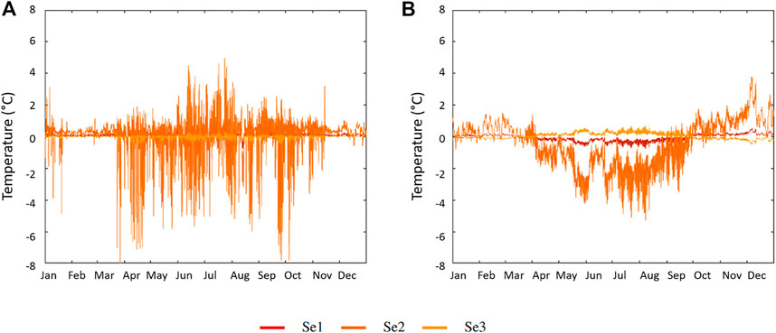
FIGURE 9. Temperature ICA component XSeC for the Sélune for typical years (A) before the dam’s removal (2014) and (B) after the dam’s removal (2020). The signal before 2019 is highly disturbed by the dam’s activity. After 2019, the signal is smoother and shows an opposite seasonal variation as the sensor was covered by sediments.
XSeC also contains a seasonal signal which stops at the dam’s removal. Such signal may be linked to the upriver lake (around 200 ha). It has a large surface exposed to atmospheric factors which can gather heat from spring to autumn and contribute to warm the Sélune. This warming is around 1.5°C in July (Figure 9A). In winter, the presence of the dam seemed to have a less significant impact even though the lake contributed to smooth and shift the phase of thermal events (Figure 10A).
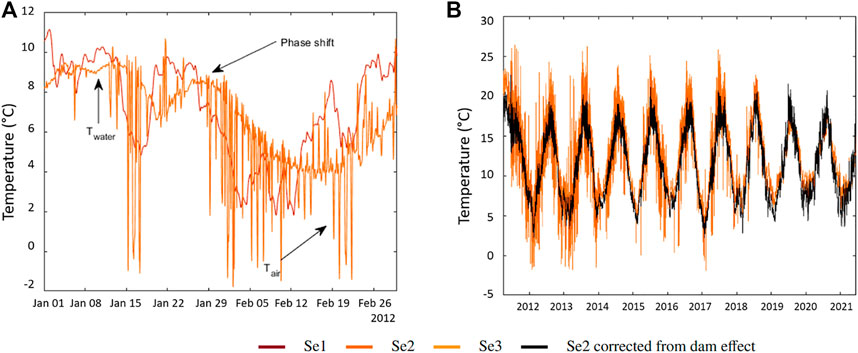
FIGURE 10. (A) Influence of hydraulic peaks on the temperature in Se2. The dam buffers the temperature amplitude and creates phase shifts. When the sensor is emerged, it measures the air temperature. (B) Temperature time series on the Sélune after removing the influence of the dam.
The main hypothesis here is that ICA gathered most of the dam’s effects in XSeC. It was confirmed by another ICA run with only XSeA and XSeB (excluding the dam’s effect in XSeC). In this second run (Figure 5), the new temperature datasets were very similar for stations Se1 and Se3 as on Figure 7, thus confirming that it was not affected by the presence or absence of the dam.
During the dam’s operation period, the production of electricity through hydraulic peaks affected the immersion of the sensor. When it was emerged, it measured Ta (Figure 10A). Indeed, if the river flow upriver the dam was low, the hydraulic head took time to come back to its original value. At these times, the electricity company EDF had to release part of the water but it was not enough to keep Se2 immersed. On the contrary, during floods (mostly in winter), the river flow could be sufficient, so EDF did not need to use hydraulic peaks. During these times, most of the upcoming river flow was released and the sensor remained immersed. Such events occurred from 2012 to 2016 (Supplementary Figure S3). In 2018, although the dam was not operating anymore, water movements previous to the dam’s removal were expressed by irregular peaks in XSeC.
After the dam’s removal (Figure 9B), XSeC shows a seasonal signal in Se3 but opposite to XSeA. This is explained by the fact that the sensor was covered by sediments after the dam’s removal and thus, the seasonal signal is strongly shifted from the atmospheric variation. Even though, it is not possible to state that the river is not affected by other dams (such as la Roche-Qui-Boit dam located between Se2 and Se3), it seems that the remaining structures do not affect the thermal regime as strongly as the Vezins dam. Using the successive ICA method described above, a reconstruction of the temperature time series without the influence of the dam (Figure 10B) was made. It shows a regular seasonal signal similar to a “natural” stream’s signal such as the Odon.
ICA extraction highlights the impact of a dam on a river and its effects on a seasonal level as well as on a daily level. In this case, the operations of the dam led to peak temperatures and a very irregular thermal regime compared to a natural river. It also led to two very different thermal regimes between the upriver station Se1 and downriver stations Se2 and Se3.
5.4 About using ICA
When analysing time series, most commonly methods such as Fourier or Morlet wavelets are frequency dependent. The initial signal is separated into several contributions based on the frequency of the phenomenon. This first approach can separate different physical phenomena which operate on very different time scale (seasonal, daily etc…). ICA, however, does not discriminate frequency scaled phenomena. Therefore, it can separate signals with similar frequency signatures. Therefore, these methods are complementary: frequency based methods are sensitive to the sampling frequency whereas ICA is sensitive to the homogeneity of the time series. The main limit of ICA lies in the separation of signals. On the two rivers, ICA could extract only three mathematically independent components on the one hand and residual signals and white noise on the other hand. Physical factors influencing the temperature are never completely independent and therefore, ICA alone can not fully separate all the contributions, unless the number of sensors is important.
However, as a first analysis step, ICA provides useful information and draws a first study frame for the physical phenomenon to look into. Also, it can be used in a backwards methodology where a factor is known to have an impact on the thermal regime but the way it impacts remains to be determined. ICA can highlight a specific signal which can be identified as the specific factor. In this study, the Vezins dam was known to influence the thermal regime of the Sélune and ICA could extract a specific signal to remove its temporary effect.
5.4.1 Contributions of ICA components
Figure 11 shows all the ICA contributions weighted by the matrix coefficients for each station. To sum up, the ICA analysis highlighted the following points:
• XOdA and XSeA (black), attributed to seasonal components, explain the majority of the rivers’ thermal signal.
• XOdB and XSeB (yellow), attributed to daily variations are regular over the years and generally stronger for upriver stations. XOdB variations correspond to a combined effect of four factors: the day/night variations, the sunlight exposition throughout the year (duration and intensity) and on top of that the vegetation’s growth and soils’ heat storage.
• XOdC and XSeC (green) contain the remainder of the temperature signal. Therefore it contains most of the particular events and local conditions affecting one station in particular. On the Odon, XOdC concerns mostly Od2 and a particularly open environment (Supplementary Figure S2). On the Sélune, XSeC concerns mostly Se2 and the effects of the Vezins dam.
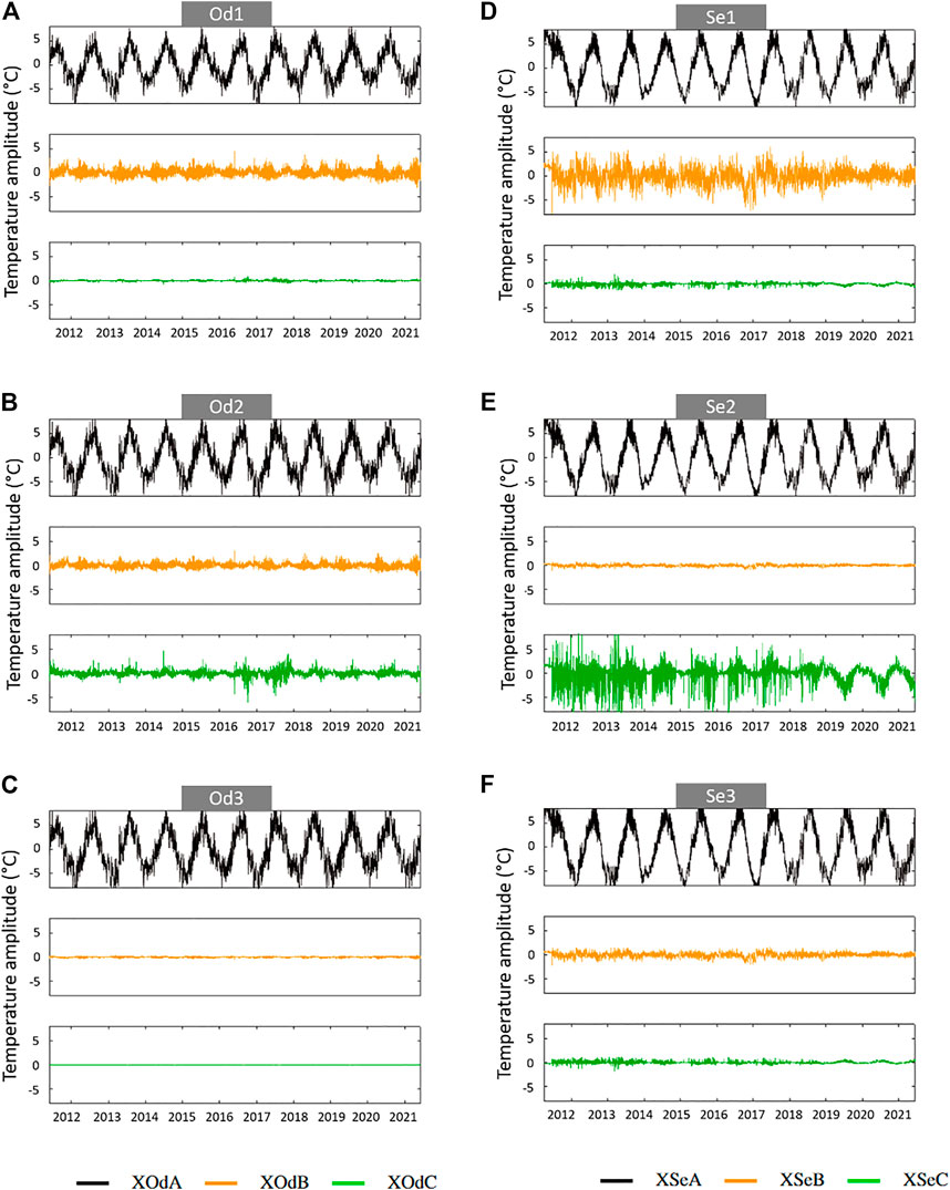
FIGURE 11. ICA components for each station of the Odon in (A–C) and the Sélune in (D–F). Seasonal components in black, daily components in yellow, specific components in green.
With this first analysis, several physical factors (climate, vegetation, soils, dam …) could be linked with ICA components and their impact evaluated according to the local context based on geology, remote sensing data, topography, land use and riparian vegetation density. However, some of known factors such as the river flow did not appear in this analysis.
5.4.2 Importance of the measuring network
ICA allowed to highlight several factors (natural or artificial) that influence the thermal regime on two rivers in Normandy. It also showed the downriver evolution of several of them.
This performance comes from the method itself but also from the measuring network which focused on less rivers but with a greater density of sensors. Ideally, five measuring sites on the Odon would have allowed to highlight the groundwater’s influence (Le Lay et al., 2019) and the impact of the distance from the sea. For the Sélune, three more stations would be necessary to study the mouth environment (1 station), the upriver basin (2 stations) which contains two main types of aquifer. Among all the measuring stations, ICA allowed to isolate the ones with specific environments. But this is only possible if the river is equipped with enough stations.
However, with a successive ICA method, more components than the number of sensors would initially allow can be extracted. ICA also gives information about the variation of the components in space (measuring stations along the river) and time. This information is useful to determine the physical factors involved.
6 Conclusion
ICA linearly decomposes the signal with the hypothesis of noise cancellation. The quality of the decomposition and the separation can be affected in the case of a strong noise. Source density under ICA is often either fixed or selected among a limited family of densities, which can cause a loss of flexibility. To counter those aspects, it could be interesting to use Independent Factors Analysis (IFA) which proposes a generative model with noise (Attias, 1999). In this model, densities are modelled with a Gaussian mix that is closer to arbitrary densities. In our case, an IFA model with time structured sources would provide further information.
In a previous paper (Gresselin et al., 2021), ICA was combined to PCA with a multiple linear regression model to characterize the respective role of groundwater and runoff in the thermal regime of a Normandy river (the Touques, France). The method has also made it possible to identify the increasing role from upstream to downstream of two climatic factors: the air temperature and the solar irradiance.
In this paper, ICA was used to characterise the influence of a hydrolelectric dam and its dismantling on the thermal regime of the Sélune (Normandy, France). ICA also identified particular periods where the sensor was covered by sediments and when it was emerged. In addition, with a new protocol called “Successive ICA”, the natural thermal regime of the river was reconstructed and testes in water temperature prediction.
On the Odon, considered as a natural river, the ICA characterized the role of the riparian vegetation and the soil on the thermal regime. The intensity of each environmental factor identified with the ICA was studied from upstream to downstream and over 10 years time.
ICA has proved the extent of its performance in classifying a wide range of control factors from a set of pre-processed time series on the one hand. On the other hand, the successive method developed here has shown its ability to remove a temporary effect, which can be useful when dealing with long-term processes. In hydrology, ICA can address at least three situations: what is the importance of other factors than the atmosphere on a river’s thermal regime? what is the evolution of a particular known factor on a river’s thermal regime? are there influencing factors that are related to one station in particular?
In Normandy for example, results produced by this study led the DREAL to create a regional map of the riparian vegetation density on the rivers’ banks (about 10 m wide on each side of the river). This map is used to determine on which stretches of watercourse the trees’ shade can be used as a limiting factor to the increasing water temperature. Such information is essential to guide decisions on river management to limit the impact of climate change (Whitehead et al., 2009; Dugdale et al., 2017).
Data availability statement
Publicly available datasets were analyzed in this study. This data can be found here: https://www.normandie.developpement-durable.gouv.fr/temperature-des-cours-d-eau-a4364.html.
Author contributions
BD and FG conceived of the presented idea. NM developed the theory and performed the computations. ZT and FG verified the analytical methods and supervised the findings of this work. All authors discussed the results and contributed to the final manuscript.
Funding
Support for this study was provided by the Agence de l’Eau Seine Normandie (Grant OPE-2020–0382).
Acknowledgments
The authors thank the Direction Régionale de l’Environnement, de l’Aménagement et du Logement (DREAL) de Normandie as well as the Office Français de la Biodiversité for the availability of the measurement data.
Conflict of interest
The authors declare that the research was conducted in the absence of any commercial or financial relationships that could be construed as a potential conflict of interest.
Publisher’s note
All claims expressed in this article are solely those of the authors and do not necessarily represent those of their affiliated organizations, or those of the publisher, the editors and the reviewers. Any product that may be evaluated in this article, or claim that may be made by its manufacturer, is not guaranteed or endorsed by the publisher.
Supplementary material
The Supplementary Material for this article can be found online at: https://www.frontiersin.org/articles/10.3389/feart.2022.1033673/full#supplementary-material
References
Aires, F., Chédin, A., and Nadal, J.-P. (2000). Independent component analysis of multivariate time series: Application to the tropical SST variability. J. Geophys. Res. 105, 17437–17455. doi:10.1029/2000JD900152
Arismendi, I., Safeeq, M., Johnson, S. L., Dunham, J. B., and Haggerty, R. (2013). Increasing synchrony of high temperature and low flow in Western north American streams: Double trouble for coldwater biota? Hydrobiologia 712, 61–70. doi:10.1007/s10750-012-1327-2
Attias, H. (1999). Independent factor analysis. Neural Comput. 11, 803–851. doi:10.1162/089976699300016458
Beaufort, A., Moatar, F., Sauquet, E., Loicq, P., and Hannah, D. M. (2020). Influence of landscape and hydrological factors on stream–air temperature relationships at regional scale. Hydrol. Process. 34, 583–597. doi:10.1002/hyp.13608
Caissie, D. (2006). The thermal regime of rivers: A review. Freshw. Biol. 51, 1389–1406. doi:10.1111/j.1365-2427.2006.01597.x
Chandesris, A., Van Looy, K., Diamond, J. S., and Souchon, Y. (2019). Small dams alter thermal regimes of downstream water. Hydrol. Earth Syst. Sci. 23, 4509–4525. doi:10.5194/hess-23-4509-2019
Comte, L., Buisson, L., Daufresne, M., and Grenouillet, G. (2013). Climate-induced changes in the distribution of freshwater fish: Observed and predicted trends. Freshw. Biol. 58, 625–639. doi:10.1111/fwb.12081
Daufresne, M., and Boët, P. (2007). Climate change impacts on structure and diversity of fish communities in rivers. Global Change Biology, Wiley 12 (13), 2467–2478.
Dugdale, S. J., Hannah, D. M., and Malcolm, I. A. (2017). river temperature modelling: A review of process-based approaches and future directions. Earth. Sci. Rev. 175, 97–113. doi:10.1016/j.earscirev.2017.10.009
Dugdale, S. J., Malcolm, I. A., Kantola, K., and Hannah, D. M. (2018). Stream temperature under contrasting riparian forest cover: Understanding thermal dynamics and heat exchange processes. Sci. Total Environ. 610-611, 1375–1389. doi:10.1016/j.scitotenv.2017.08.198
Ebersole, J. L., Liss, W. J., and Frissell, C. A. (2001). Relationship between stream temperature, thermal refugia and rainbow trout Oncorhynchus mykiss abundance in arid-land streams in the northwestern United States. Ecol. Freshw. Fish. 10, 1–10. doi:10.1034/j.1600-0633.2001.100101.x
Evans, E. C., McGregor, G. R., and Petts, G. E. (1998). River energy budgets with special reference to river bed processes. Hydrol. Process. 12, 575–595. doi:10.1002/(SICI)1099-1085(19980330)12:4⟨575:AID-HYP595⟩3.0.CO;2-Y
Garner, G., Malcolm, I. A., Sadler, J. P., and Hannah, D. M. (2017). The role of riparian vegetation density, channel orientation and water velocity in determining river temperature dynamics. J. Hydrol. X. 553, 471–485. doi:10.1016/j.jhydrol.2017.03.024
Gong, W., Yang, D., Gupta, H. V., and Nearing, G. (2014). Estimating information entropy for hydrological data: One-dimensional case. Water Resour. Res. 50, 5003–5018. doi:10.1002/2014WR015874
Gresselin, F., Dardaillon, B., Bordier, C., Parais, F., and Kauffmann, F. (2021). Use of statistical methods to characterize the influence of groundwater on the thermal regime of rivers in normandy, France: Comparison between the highly permeable, chalk catchment of the touques river and the low permeability, crystalline rock catchment of the orne river. Geol. Soc. Lond. Spec. Publ. 517 (1), SP517-2020-117. doi:10.1144/SP517-2020-117
Hannachi, A., Unkel, S., Trendafilov, N. T., and Jolliffe, I. T. (2009). Independent component analysis of climate data: A new look at eof rotation. J. Clim. 22, 2797–2812. doi:10.1175/2008JCLI2571.1
Hannah, D. M., and Garner, G. (2015). River water temperature in the United Kingdom: Changes over the 20th century and possible changes over the 21st century. Prog. Phys. Geogr. Earth Environ. 39, 68–92. doi:10.1177/0309133314550669
Hyvärinen, A., and Oja, E. (2000). Independent component analysis: Algorithms and applications. Neural Netw. 13, 411–430. doi:10.1016/S0893-6080(00)00026-5
Jackson, F., Hannah, D. M., Fryer, R., Millar, C., and Malcolm, I. (2017). Development of spatial regression models for predicting summer river temperatures from landscape characteristics: Implications for land and fisheries management. Hydrol. Process. 31, 1225–1238. doi:10.1002/hyp.11087
Johnson, M. F., Wilby, R. L., and Toone, J. A. (2013). Inferring air-water temperature relationships from river and catchment properties: AIR-WATER temperature relationships in rivers. Hydrol. Process. 28 (6). doi:10.1002/hyp.9842
Jones, N. E., and Schmidt, B. J. (2018). Thermal regime metrics and quantifying their uncertainty for north American streams. River Res. Appl. 34, 382–393. doi:10.1002/rra.3257
Kelleher, C., Wagener, T., Gooseff, M., McGlynn, B., McGuire, K., and Marshall, L. (2012). Investigating controls on the thermal sensitivity of Pennsylvania streams. Hydrol. Process. 26, 771–785. doi:10.1002/hyp.8186
Lalot, E., Curie, F., Wawrzyniak, V., Baratelli, F., Schomburgk, S., Flipo, N., et al. (2015). Quantification of the contribution of the beauce groundwater aquifer to the discharge of the loire river using thermal infrared satellite imaging. Hydrol. Earth Syst. Sci. 19, 4479–4492. doi:10.5194/hess-19-4479-2015
Larnier, K., Roux, H., Dartus, D., and Croze, O. (2010). Water temperature modeling in the garonne river (France). Knowl. Manag. Aquat. Ecosyst. 04, 04. doi:10.1051/kmae/2010031
Le Lay, H., Thomas, Z., Rouault, F., Pichelin, P., and Moatar, F. (2019). Characterization of diffuse groundwater inflows into stream water (Part II: Quantifying groundwater inflows by coupling FO-dts and vertical flow velocities). Water 11, 2430. doi:10.3390/w11122430
Magnuson, J. J., Crowder, L. B., and Medvick, P. A. (1979). Temperature as an ecological resource. Am. Zool. 19, 331–343. doi:10.1093/icb/19.1.331
Marchini, J. L., Heaton, C., and Ripley, B. D. (2001). Maintainer and Algorithm, Fastica. The fastICA Package.
Middleton, M. A., Whitfield, P. H., and Allen, D. M. (2015). Independent component analysis of local-scale temporal variability in sediment-water interface temperature: Ica to examine sediment-water. Water Resour. Res. 51, 9679–9695. doi:10.1002/2015WR017302
Moatar, F., and Gailhard, J. (2006). Water temperature behaviour in the river loire since 1976 and 1881. Comptes Rendus Geosci. 338, 319–328. doi:10.1016/j.crte.2006.02.011
Moradkhani, H., and Meier, M. (2010). Long-lead water supply forecast using large-scale climate predictors and independent component analysis. J. Hydrol. Eng. 15, 744–762. doi:10.1061/(ASCE)HE.1943-5584.0000246
Poirel, A., Lauters, F., and Desaint, B. (2008). 1977-2006: Trente années de mesures des températures de l’eau dans le bassin du rhône. Hydroecol. Appl. 16, 191–213. doi:10.1051/hydro/2009002
Poirel, J., Gailhard, J., and Capra, H. (2010). Influence des barrages-réservoirs sur la température de l’eau : Exemple d’application au bassin versant de l’ain. La Houille Blanche 4, 7279–79. doi:10.1051/lhb/2010044
Poole, G. C., and Berman, C. H. (2001). An ecological perspective on in-stream temperature: Natural heat dynamics and mechanisms of human-CausedThermal degradation. Environ. Manage. 27, 787–802. doi:10.1007/s002670010188
Ryan, D. K., Yearsley, J. M., and Kelly-Quinn, M. (2013). Quantifying the effect of semi-natural riparian cover on stream temperatures: Implications for salmonid. habitat Manag. 20, 494–507. doi:10.1111/fme.12038
Seyedhashemi, H., Moatar, F., Vidal, J.-P., Diamond, J. S., Beaufort, A., Chandesris, A., et al. (2021). Thermal signatures identify the influence of dams and ponds on stream temperature at the regional scale. Sci. Total Environ. 766, 142667. doi:10.1016/j.scitotenv.2020.142667
Sinokrot, B. A., and Stefan, H. G. (1994). Stream water?temperature sensitivity to weather and bed parameters. J. Hydraul. Eng. 120, 722–736. doi:10.1061/(asce)0733-9429(1994)120:6(722)
Souchon, Y., and Tissot, L. (2012). Synthesis of thermal tolerances of the common freshwater fish species in large Western Europe rivers. Knowl. Manag. Aquatic Ecosyst. 405 (405). doi:10.1051/kmae/2012008
Torgersen, C. E., Faux, R. N., McIntosh, B. A., Poage, N. J., and Norton, D. J. (2001). Airborne thermal remote sensing for water temperature assessment in rivers and streams. Remote Sens. Environ. 76, 386–398. doi:10.1016/S0034-4257(01)00186-9
Webb, B., and Walling, D. (1993). Temporal variability in the impact of river regulation on thermal regime and some biological implications. Freshw. Biol. 29, 167–182. doi:10.1111/j.1365-2427.1993.tb00752.x
Webb, B. W., Hannah, D. M., Moore, R. D., Brown, L. E., and Nobilis, F. (2008). Recent advances in stream and river temperature research. Hydrol. Process. 22, 902–918. doi:10.1002/hyp.6994
Westra, S., Sharma, A., Brown, C., and Lall, U. (2008). Multivariate streamflow forecasting using independent component analysis. Water Resour. Res. 44. doi:10.1029/2007WR006104
Keywords: river temperature, time series analysis, ICA, river management, water temperature prediction, dam removal influence, riparian vegetation
Citation: Moulin N, Gresselin F, Dardaillon B and Thomas Z (2022) River temperature analysis with a new way of using Independant Component Analysis. Front. Earth Sci. 10:1033673. doi: 10.3389/feart.2022.1033673
Received: 31 August 2022; Accepted: 24 November 2022;
Published: 14 December 2022.
Edited by:
Celso Santos, Federal University of Paraíba, BrazilReviewed by:
Didier G. Leibovici, The University of Sheffield, United KingdomAznarul Islam, Aliah University, India
Copyright © 2022 Moulin, Gresselin, Dardaillon and Thomas. This is an open-access article distributed under the terms of the Creative Commons Attribution License (CC BY). The use, distribution or reproduction in other forums is permitted, provided the original author(s) and the copyright owner(s) are credited and that the original publication in this journal is cited, in accordance with accepted academic practice. No use, distribution or reproduction is permitted which does not comply with these terms.
*Correspondence: Nelly Moulin, bmVsbHkubW91bGluQGluc3RpdHV0LWFncm8uZnI=; Zahra Thomas, emFocmEudGhvbWFzQGluc3RpdHV0LWFncm8uZnI=