 Malcon Celorio
 Emmanuel Chaljub
 Ludovic Margerin3
- 1Univ. Grenoble Alpes, Univ. Savoie Mont Blanc, CNRS, IRD, Univ. Gustave Eiffel, ISTerre, Grenoble, France
- 2Grupo Quimbaya, CEIFI, Observatorio Sismológico Universidad del Quindío, Armenia, Colombia
- 3Institut de Recherche en Astrophysique et Planétologie, Observatoire Midi-Pyrénées, Université Paul Sabatier, CNRS, Toulouse, France
Increasing the frequency range of physics-based predictions of earthquake ground motions requires to account for small-scale heterogeneities, which can only be described in a stochastic way. Although many studies have addressed the impact of random heterogeneities on ground motion intensity parameters obtained by numerical simulation, very few have verified the accuracy of their numerical solutions or controlled the scattering regime they were simulating. Here we present a comprehensive analysis of SH wave propagation in 2D random media which covers a broad range of propagation regimes from ballistic to diffusive. The coherent and incoherent parts of the wavefield are examined independently. The random media consist in correlated density and velocity fluctuations described by a von Kármán autocorrelation function with a Hurst coefficient of 0.25 and a correlation length a = 500 m. The Birch correlation coefficient which relates density to velocity fluctuations takes 4 possible values between 0.5 and 1, and the standard deviation of the perturbations is either 5% or 10%. Spectral element simulations of SH wave propagation excited by a plane wave are performed for normalized wavenumbers (ka) up to 5. Analysis of the decay of the coherent wave amplitude, obtained through different averaging procedures, allows for a direct measure of the scattering attenuation, which we successfully compare with the predictions of the Dyson mean field theory. We also present the comparison between the energy envelopes measured from the synthetics and their theoretical counterpart provided by the radiative transfer theory and the diffusion approximation. Excellent agreement is found between numerical simulations and theoretical predictions of radiative transfer theory for the mean intensity. The numerical study highlights the difference of attenuation length between the mean field and the mean intensity. In the forward scattering regime, the peak intensity appears to decay exponentially over a length scale known as the transport mean free path. Furthermore, the fluctuations of intensity in the ballistic peak exhibit a transition from Log-normal to Exponential statistics. This transition occurs for a propagation distance of the order of the mean free path, which offers an alternative method of estimating this parameter.
1 Introduction
Heterogeneities exist at all scales in the Earth (Sato, 2019) and have to be taken into account for a realistic estimation of earthquake ground motions (e.g., Imperatori and Mai, 2012; Takemura et al., 2015; Hu et al., 2022). In the range of frequencies considered in seismic hazard assessment (up to few tens of Hz), the shortest S wavelengths vary from hundreds of metres, in the source region, to tens of metres, in the near-surface sedimentary layers. Accounting for the heterogeneities that influence the propagation of those wavelengths is critical and poses a number of difficulties for physics-based approaches. First, the description of these small-scale heterogeneities cannot be deterministic. In the current state-of-practice, the propagation media are usually considered as random and several realisations have to be considered to obtain robust estimates of the effect of the heterogeneities on seismic wave propagation. This represents a significant additional computational cost for grid-based approaches such as finite difference or finite element methods. Second, the statistical properties of small-scale heterogeneities can only be constrained from rare direct near-surface measurements (Wu et al., 1994; Holliger, 1996; Shiomi et al., 1997; Dolan et al., 1998), and more generally have to be inferred from their (cumulative) effect on recorded seismic waveforms, from the ballistic phases to the seismic coda. This in turn requires the use of specific methods capable of extracting statistical information on the propagation medium without relying on the computation of full waveforms.
The problem of recovering the characteristics of small-scale heterogeneities is common to different branches of applied physics such as non-destructive evaluation, medical and seismic imaging, to cite a few examples only. In all these fields, radiative transfer theory (RTT, also known as transport theory) has emerged as a key tool for modeling and inverting for the scattering and absorption properties of media with micro-structure (Turner and Weaver, 1994; Margerin, 2005; Arridge and Schotland, 2009). RTT models the transport of energy in heterogeneous media based on the two-point correlation function of the fluctuations in elastic parameters. As such, it only describes the modulation of the envelope of the seismic signals but does not provide information on the details of the waveforms. Correlation functions of the von Kármán type have been almost universally adopted in seismological studies. They provide reasonable representations of the small-scale fluctuations in the Earth (see Sato, 2019, for a review) with the aid of only three parameters: correlation length, standard deviation of the fluctuations and Hurst exponent controlling the distribution of the variance over all possible length scales. While originally introduced on a phenomenological basis (e.g., Chandrasekhar, 1960; Wu, 1985; Zeng, 1993; Sato, 1994), RTT has nowadays acquired solid theoretical foundations. In particular, transport equations for elastic waves have been derived in infinite space based on multiple scattering theories (Weaver, 1990) or two-scale expansion methods (Ryzhik et al., 1996). In spite of this great simplification of the physics, the radiative transfer equation (RTE) has the reputation of being notoriously difficult to solve. Indeed, only a few analytical solutions for canonical cases can be found in the literature (Paasschens, 1997). Fortunately, with nowadays computational power, Monte-Carlo (MC) simulations offer a convenient tool to produce numerical solutions in a variety of cases of seismological interest (Shearer and Earle, 2004; Sanborn et al., 2017). In seismology, RTT is still an active area of research. A currrent Frontier in the field concerns the coupling between surface and body waves which occurs in the vicinity of the free surface in a half-space or slab geometry (Tregoures and Van Tiggelen, 2002; Margerin et al., 2019; Borcea et al., 2021; de Hoop et al., 2022; Xu et al., 2022). Another topic of interest is the treatment of random media with a correlation length which is large compared to the wavelength. Because it relies on a perturbative approach (Born approximation), the transport equations for continuous random media found in the literature break down in the high-frequency (geometrical optics) limit. Sato and Emoto (2018) proposed to remedy this deficiency by dividing the power spectrum into a short-scale and a long-scale component. The former is treated via the traditional Born approximation and the latter by the phase screen approximation. The theory involves a free parameter which separates the short- and long-scale components, which is determined by comparisons between MC simulations of the transport process and envelopes obtained from waveform simulations using the finite difference method. The work of Sato and Emoto (2018) provides a concrete illustration of the key interplay between simulations of wave propagation in random media and MC simulations in the development and validation of transport theory (see also Przybilla et al., 2006; Wegler et al., 2006; Przybilla and Korn, 2008).
Direct (ab initio) numerical simulation of seismic wave propagation offer the possibility to consider arbitrarily complex random media (for example heterogeneous background media, composite random fluctuations) and to explore different scattering regimes and their transitions without approximations. With the advent of mature computational codes and the computational power available, it is now feasible to simulate tens of realizations of 3D random media in realistic ranges of size and frequency and to perform comprehensive parametric studies in 2D. Since the pioneering article of Frankel and Clayton (1986), many studies have exploited the potential of numerical simulation to predict the effect of random heterogeneities on the seismic wavefield. The impact of scattering by heterogeneities, in the crust or in near-surface sedimentary layers, on the prediction of earthquake ground motion is nowadays an active field of research (Hartzell et al., 2010; Imperatori and Mai, 2012; Imperatori and Mai, 2015; Takemura et al., 2015; Savran and Olsen, 2019; Scalise et al., 2021; Tchawe et al., 2021; van Driel et al., 2021; Hu et al., 2022). However, despite considerable efforts to account for scattering in the estimation of ground motion, many of the results presented in these numerical studies are difficult to appreciate or to extrapolate because i) they often lack a verification phase to ensure that the targeted random media are well implemented and ii) the scattering regimes considered are not sufficiently described to allow for unambiguous physical interpretation. This last point is particularly critical since inversion of scattering and absorption properties based on RTT cannot resolve the full power spectrum of heterogeneities but provide instead scale lengths characterizing the propagation regime such as the scattering mean free path or even more appropriately the transport mean free path (Gaebler et al., 2015). As further documented in the rest of the paper, these quantities control the main characteristics of the seismogram envelopes (see also Sato et al., 2012). We therefore argue that realistic simulations of ground motions should target specific value for the scattering mean free paths rather than ad-hoc or a priori estimates for the correlation length and variance of small-scale heterogeneities.
In this article, we present a comprehensive analysis of the propagation of SH waves in 2D random media by combining ab initio numerical simulation and RTT. This simple physical setting allows us to consider a large set of von Kármán random media and to simulate wave propagation in a broad range of frequency and propagation regimes, from ballistic to diffusive. We believe that our study is unprecedented in this respect. We carefully verify the implementation of the random media by comparing direct measures of the scattering mean free path to their theoretical estimates. This part of the study relies on different methods for averaging the wavefield. We discuss in detail the role of spatial vs. ensemble averaging, considering a number of realizations of the random media which has no equivalent in previous studies. In the second part of the work, the mean intensities derived from the numerical simulations are compared to those predicted by RTT as proposed by several authors [e.g., Przybilla et al. (2006), Emoto and Sato (2018)]. We pay particular attention to the apparent attenuation of the ballistic peak of seismic waves, which is a key parameter in seismic hazard evaluation. The attenuation study is complemented with an analysis of the fluctuations of the ballistic intensity. The combination of the two viewpoints provides insight into the evolution of the ballistic peak with propagation distance and illustrates the transitions between different propagation regimes.
The organisation of the manuscript is as follows: Section 2 provides a review of useful concepts to address wave propagation in random media, in particular mean field and radiative transfer theories, and presents the collection of data sets obtained by numerical simulation. Comprehensive analyses of the results obtained by transport theory and numerical simulations are shown in Section 3 and followed by some conclusions in Section 4.
2 Materials and methods
2.1 Wave propagation in random media
In this work, we consider the propagation of a scalar wavefield u governed by the 2-D elastodynamic Equation in anti-plane geometry:
where µ and ρ denote, respectively, the rigidity and density of the medium and x is the position vector.
The symbol f (t, x) represents an external source. The local velocity is defined by
In Eq. 2,
where ρ0 is the ensemble average density and ν is a scaling factor between density and velocity fluctuations known as Birch coefficient (Sato et al., 2012). In Earth’s crust, the correlation between velocity and density is broadly supported by borehole observations (e.g., Shiomi et al., 1997). To lowest order in perturbations, scattering in disordered media is governed by the correlation properties of the disorder. For the representation of random elastic fluctuations in seismology, the most widely accepted form of auto-correlation function R is of von Kármán type:
where r = |r| and the brackets ⟨⟩ indicate an ensemble average, i.e., an average over an infinite sample of realizations of random media sharing the same correlation properties. In Eq. 4, a is the correlation length of the fluctuations, H represents the Hurst exponent, Γ(H) is the Gamma function and KH is the modified Bessel Function of order H. Note that the definition (Eq. 4) implies spatial stationarity (or statistical uniformity) as well as isotropy of the random fluctuations. The Fourier Transform of R is the power spectral density of fluctuations also termed heterogeneity power spectrum P. In the case of von Kármán media, it is given by:
By isotropy, P depends only on the modulus of the wavenumber of the fluctuations (k = |k|). The power spectrum (Eq. 5) exhibits power-law behavior for length scales 2π/k (much) smaller than the correlation length a. This behavior is largely supported by direct measurements of velocity and density fluctuations over a broad range of scales ranging from rock samples in the laboratory to logging data in boreholes (see Sato, 2019, for a review). The broadband nature of heterogeneity in geological materials is a challenge for seismic wavefields computations in seismology. As an example, popular numerical methods such as finite difference or finite elements require the artificial introduction of a cut-off wavenumber kc beyond which the power spectrum is assumed to be 0 (i.e., P (k) = 0 for k ≥ kc). For comparison with seismic data, it is important to assess the effects of cut-offs on the computed wavefield. More generally, it is crucial to control the level of scattering produced by small-scale heterogeneities in numerical models. Indeed, scattering is a key process controlling the attenuation of direct waves, the broadening of seismograms and the fluctuations of waveforms. In what follows, we briefly summarize the main ingredients and predictions of transport methods and refer the reader to Weaver (1990), Ryzhik et al. (1996) for in-depth derivations.
2.2 Mean field theory
One of the most well-known and important manifestation of scattering by small scale heterogeneities is the attenuation of direct waves. There exists a variety of approaches to measure direct wave attenuation that lead to significantly different estimates (e.g., Sato, 1982; Wu, 1982), possibly also dependent on the observation scale (Shapiro and Kneib, 1993). From the theoretical point of view, the simplest quantity to be derived from simulations of wave propagation in random media is the ensemble average field ⟨u(x)⟩. This quantity is also called the coherent field since the averaging procedure selects the portion of the wavefield that has maintained the exact same propagation direction from emission to detection. The part of the wavefield that has been scattered at least once sees its phase fluctuate randomly from realization to realization and is eliminated by ensemble averaging. The mean field is governed by the Dyson equation (Frisch, 1968; Rytov et al., 1989) whose solution predicts an exponential decay of the coherent amplitude with a length scale known as the scattering mean free path ℓ. The scattering mean free path is a central quantity in transport theory as it also represents the mean distance between two scattering events for multiply-scattered waves.
The exact solution of the Dyson Equation is available only in simple cases such as scalar waves in exponentially correlated random media (corresponding to the Hurst exponent H = 1/2). Fortunately, the mean free path may be approximately evaluated by applying the Born approximation to the calculation of the mean energy scattered off a plane wave incident on a representative elementary volume of random medium (REV) embedded in an otherwise homogeneous background with density ρ0 and velocity v0 (Sato, 1984). The typical linear dimension L of the REV should fulfill the scaling conditions a ≪ L ≪ ℓ which guarantees that it contains a large number of heterogeneities yet only scatters a small fraction of the energy of the incident wave. By normalising the energy scattered per unit time by the volume of the REV and the incident energy flux of the plane wave, one obtains an estimation of the scattering attenuation (in km−1) or inverse mean free path (ℓ−1). This heuristic method is valid only for sufficiently low frequencies (ωa
Following the heuristic method outlined above, the following general expression for the scattering attenuation in 2-D antiplane geometry is obtained:
where
Making use of Birch law and assuming random media of von Kármán type, Eq. 6 leads to:
where θ denotes the scattering angle. From Eq. 7 the scattering attenuation may be easily evaluated numerically. To gain insight into the frequency dependence of scattering attenuation we provide some simple approximations to ℓ−1 in the low- and high- frequency regimes. In the case (kβa ≪ 1), the denumerator of the integrand in (Eq. 7) may be approximated by the constant 1 over the full range of integration. In such a case the angular dependence is entirely governed by the numerator which directly depends on the nature of the elastic perturbations, i.e., on the particular form of correlations among the elastic parameters ρ and β. In the case of the Earth, the two quantities are generally positively correlated, so that scatterers present contrasts of impedance with respect to the background medium. This gives rise to large lobes of scattering in the backward direction. After a simple integration of the trigonometric polynomial, one finds:
The cubic frequency dependence is characteristic of the so-called Rayleigh regime in 2-D, corresponding to wavelengths much larger than the size of the scatterers. In the intermediate frequency regime, also known as stochastic regime (Stanke and Kino, 1984), we remark that the integrand is the product of a smooth function (numerator) times a function which is sharply peaked in a cone of typical angular width θ = O (1/kβa) around θ = 0. Based on these observations, we perform the following approximations (Yang et al., 2011): (1) replace the numerator by its value at θ = 0, (2) substitute sin (θ/2) with θ/2 in the denominator, (3) introduce the new variable ψ = kβaθ and integrate from ψ = −∞ to ψ = +∞. After application of this procedure, one obtains:
Hence, in the frequency regime where the wavelength is of the order of (or smaller than) the size of the scatterers, attenuation is found to grow like ω2. In 3-D, attenuation exhibits the same frequency dependence in the stochastic regime as in 2-D so that the transition from low to high frequencies is far more visible in the former situation. Let us finally remark that (Eq. 9) is deceptively simple since it suggests that scattering attenuation is independent of the Birch parameter ν. There are in fact corrections terms to (Eq. 9) that depend on ν. This will become apparent when we consider applications to different types of random media. The asymptotic dependencies predicted by (Eqs 8, 9) are compared to the exact solution of (Eq. 6) in Figure 1 for a von Kármán medium with correlation length a = 500 m, Birch coefficient ν = 1 and standard deviation of the fluctuations 5%.
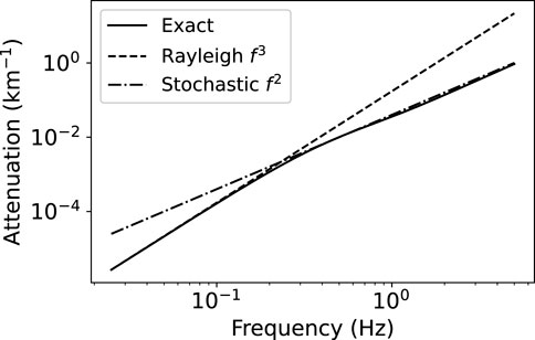
FIGURE 1. Rayleigh and stochastic regimes in scattering attenuation.
In seismology, the ensemble averaging procedure is somewhat out of reach experimentally. Even if seismic stations were readily movable, one would still have to assume that the underlying medium is statistically homogeneous, which is difficult to control. Hence, we have to accept that seismic measurements always mix the coherent, mean wave with the incoherent, scattered waves. By considering the second moment of the field, i.e., the energy density carried by the waves, transport (or radiative transfer) theory provides a consistent framework to treat on the same footing the coherent and incoherent parts of the wavefields. A brief summary of this approach is provided in the next section.
2.3 Transport theory
Transport equations describe the ensemble average propagation of energy density in a random medium. They may be derived from the wave equation by considering the statistical mean of Wigner distribution of the wavefield in the limit where temporal and spatial scales are both well separated. This means that one considers the slow temporal modulation of fields that rapidly oscillates at the central frequency ω. Analogously, in the spatial domain, one imagines wave packets with a slowly varying envelope that modulates the amplitude of short wavelength oscillations (λ = 2πc0/ω). We refer the reader to the classical papers by Weaver (1990) and Ryzhik et al. (1996) for in-depth treatments based on statistical physics and mathematical approaches, respectively. Here we simply recall the form of the transport Equation:
where the following notations have been introduced: c, the wave velocity,
with C a normalization factor which depends on the wave type. (Eq. 11) defines the specific energy density as the angular power spectral density of the wavefield at time t, position r and frequency ω, implicit in the left-hand side of Eq. 11. Note that the wavefield u has been filtered in a narrow frequency band of interest beforehand. More will be said on this point in Section 3.2.1. The time-frequency representation of e is key in transport theory, since as illustrated in the previous section, the scattering mean free time τ depends strongly on the frequency of the propagating waves. Note that the dependence of τ on ω is implicit in (Eq. 10). Similarly, the position-wavenumber representation enables one to take into account the angular dependence of the scattering. More precisely, the probability for a wave propagating in direction
with N a normalization constant such that
As outlined above, the multiple-scattering process tends to randomize the directions of propagation in the random medium. Hence, we may expect that at sufficiently long lapse time the specific intensity departs only slightly from isotropy. When this regime sets in, a diffusion Eq. for the energy density integrated over all propagation directions [e (t, r)] can be derived from the RTE (e.g. Kourganoff, 1969; Weaver, 1990):
where the diffusion constant in 2-D is defined as:
The formula for the diffusivity of seismic waves features the transport mean free path ℓ∗ as a new length scale:
Comparing (Eqs 15, 7), we may write ℓ∗ = ℓ/(1−g) where g is the mean cosine of the scattering angle. Physically, ℓ∗ represents the propagation distance required to randomize the propagation direction of a plane wave incident on the random medium. In the Rayleigh regime, backscattering is dominant (g < 0) and the transport mean free path is generally smaller than the scattering mean free path. Note that ℓ∗ is always greater than ℓ/2 so that the two length scales do not differ very much in the low-frequency regime. The formula analogous to (Eq. 8) for the transport mean free path is given by:
When one approaches the stochastic regime, the scattering pattern becomes more and more strongly peaked in the forward direction. In the high-frequency limit, g approaches 1 and the transport mean free path can largely exceed the scattering mean free path. The simple method used to obtain an asymptotic expansion of ℓ in the stochastic regime cannot be applied to obtain an estimate of ℓ∗ because the (1−cos θ) term in the numerator of (Eq. 15) evaluates to 0 in the forward direction. In the exponential case used for the numerical simulations, it is possible to obtain closed form expressions for the transport mean free path using symbolic computation softwares such as Mathematica™ but the final formulas are not particularly illuminating. Nevertheless, their expansion for large ka suggests that the transport mean free path increases logarithmically for large ka. Note that this result is specific to the case κ = 1/2. The key message here is that the frequency dependence of the transport mean free path contains information on the Hurst exponent.
The diffusion model would not be complete without the prescription of the initial and boundary conditions. In the numerical simulations, we consider a plane wave incident in direction ˆz on a slab of random medium of thickness H with absorbing conditions at the top (z = 0) and bottom (z = H). Adapting the method of (Zhu et al., 1991) to the 2-D case, we find that the diffuse energy density should satisfy the following set of boundary conditions:
with x the coordinate perpendicular to z [r = (x, z)]. For the initial condition, we simply consider that the total energy is injected diffusively at a distance ℓ∗ from the lower boundary at time t = t∗ (with t = 0 the time at which the incident plane wave enters the random medium). By diffuse injection, we mean that the initial direction of energy propagation is uniformly distributed in [0, 2π]. In spite of its crudeness, this approximation gives satisfactory results in many cases of interest.
2.4 Numerical modelling: SEM solution
Numerical simulations of SH wave propagation in 2D elastic random media are performed with the specfem2D code, which implements the Spectral Element Method (SEM, e.g., Komatitsch and Vilotte (1998), Chaljub et al. (2007)) in space and a second order finite difference scheme in time. The computational domain consists of a square of size L = 314 km with periodic conditions on the lateral edges and absorbing conditions on the upper and lower edges. The domain is meshed with 106 squared elements of size 314 m and an order N = 4 is used to define the local polynomial bases. Random media are defined by superimposing velocity and density fluctuations on a homogeneous background medium with shear wave velocity V0 = 3.14 km s−1 and density ρ0 = 2,500 kg m−3. The fluctuations of density are correlated to those of velocity through dρ/ρ0 = ν dV/V0, where ν is the Birch coefficient which we restrict to the four possible values: 0.5, 0.67, 0.8, and 1. The fluctuations are further defined by a von Kármán auto-correlation function (ACF) with typical crustal values: correlation length a = 500 m, Hurst exponent κ = 0.25, and standard deviation ε = 5% or 10%. Eight different random media are therefore considered corresponding to the four values of ν and the two values of ε. The implementation of the fluctuations follows the classical spectral approach (see e.g., Sato et al. (2012)): the fluctuations are first defined in the Fourier domain from the square root of the modulus of the ACF as the amplitude spectrum (according to Eq. 5) and a uniformly distributed random phase, then transported back to the spatial domain by the inverse Fourier transform. Finally, we apply a cosine taper on the fluctuations along a 5 km thick layer as we approach the lateral edges in order to be consistent with the periodic boundary conditions. Note that with our choice of the background velocity and of the correlation length, the normalized wavenumber ka, which characterizes the scattering regime, is equal to the frequency f.
The interaction of a given seismic wavelength λ with the random medium requires all heterogeneities with size larger than λ/2 to be well discretized (see Section 2.2). Assuming a minimum of 5-6 points per seismic wavelength, this requirement is naturally satisfied (with 2.5–3 points) but fluctuations with size smaller than λ/2 have to be eliminated first in order to avoid spatial aliasing at the discrete level. This is achieved by applying a (4 poles, 2 passes) Butterworth low-pass filter (below ka = 10) to the ACF before the inverse Fourier transform. With this choice of the discretization parameters, we consider that the propagation of SH waves in random media is accurately simulated for frequencies up to at least 5 Hz. An example of realization of random fluctuations, corresponding to standard deviation ε = 5%, is given in Figure 2A. Note that for subsequent analyses which require ensemble averages, we performed 60 realizations of each of the eight random media. The media are further excited by a plane wave with vertical incidence. The choice of the plane wave is intended to simplify subsequent analyses of amplitude decay with distance since no geometrical spreading needs to be considered. For each of the 480 simulations, we record the particle velocity at three sets of receivers, Wi, Ci and Ei, located at the same vertical position Zi and separated by 50 km in the horizontal direction (see Figure 2B).
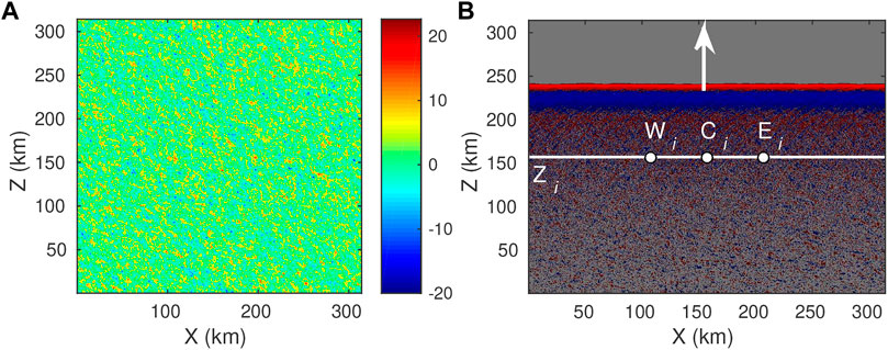
FIGURE 2. (A) 2D fluctuations defined by a von Kármán ACF with correlation length 500 m, Hurst exponent 0.25 and standard deviation 5%. The colorbar indicates the amplitude of the fluctuations in %. (B) snapshot of an up-going plane wave in the random medium with a Birch coefficient ν = 1. Red/blue colors indicate positive/negative particle velocity. At a given propagation distance Zi, 3 receivers are defined: Wi (west), Ci (centre) and Ei (east).
Different averages will be considered for each random medium and each vertical position Zi: i) ensemble average, corresponding to the average over the three receivers Wi, Ci and Ei (considered as independent) and over the 60 realizations of the random medium; ii) horizontal spatial average, corresponding to the average over all (about 5,000) Gauss-Lobatto-Legendre gridpoints located at vertical position Zi (white line in Figure 2B); iii) ensemble-space average corresponding to the average over the 60 realizations of the horizontal spatial average.
For the source time function, we use a Dirac delta function which we band-pass filter between 10−1 Hz and 8 Hz with Butterworth filters of different orders (see Figure 3A).
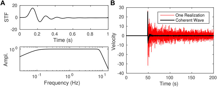
FIGURE 3. (A) source time function (top) with its Fourier amplitude spectrum (bottom) showing energy uniformly distributed between 0.1 Hz and 8 Hz. (B) particle velocity obtained after 150 km of propagation for a single realization of the random medium of Figure 2. The red curve corresponds to a single receiver whereas the black curve corresponds to the spatial average along the horizontal white line of Figure 2B.
The red trace in Figure 3B shows an example of particle velocity recorded at z = 150 km for one realization of the random medium of Figure 2. The black trace corresponds to the coherent wave, which is obtained here as the space average at distance z.
3 Results
3.1 Mean wavefield scattering attenuation
The scattering attenuation can be estimated directly from the amplitude decay of the coherent wave with distance. The measurement process is illustrated in Figure 4 for the random medium of Figure 2. The top figures show the seismic sections for the central receivers Ci (left) and for the coherent wave (right). The Fourier amplitude of the coherent wave is displayed as a function of frequency for different distances (bottom left) and as a function of distance for different frequencies (bottom right). From the latter, we measure at each frequency, f, the scattering mean free path, ℓ(f), by fitting an exponential decay exp [−z/2ℓ(f)]. Note that as the propagation distance and frequency increase, the Fourier amplitude may decrease so much that the measurement of the decay is no longer robust. In such case, we use a threshold value for the amplitude which is around 5% and 15% of the maximum amplitude and chosen by visual inspection. Note also that the coherent wavefield used in Figure 4 is obtained by ensemble-space averaging. Corresponding figures for the other averages (space, ensemble) are presented in Supplementary Figure S1 of the supplementary material.
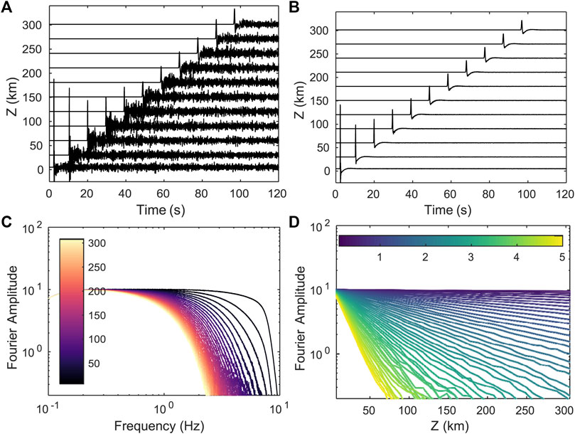
FIGURE 4. Waveforms and Fourier spectra for the case ν = 1 and ε = 5%. Top: seismic sections of particle velocity for one single realization (A) and for the coherent wavefield obtained by ensemble-space average (B) Bottom: Fourier amplitude spectra of the coherent wavefield as a function of frequency (C) and source-receiver distance (D) Color bars represent the range of propagation distance and frequency, respectively.
The estimates of scattering attenuation, defined as the inverse of the scattering mean free path, ℓ−1 (f), are shown in Figure 5 as a function of frequency. For each of the eight random media, different estimates are shown, corresponding to different averaging procedures used to define the coherent wavefield: dotted lines correspond to the ensemble average, dashed lines to the space average and solid lines to the ensemble- space average. Results were obtained in the frequency range between 0.1 and 5 Hz with a step of 0.1 Hz. As can be seen, the ensemble average can not be used beyond 3 Hz (resp. 1 Hz) for fluctuations standard deviation ε = 5% (resp. ε = 10%). The horizontal space average, obtained for a single realization of each random medium, yields robust estimates for all cases with ε = 5% but cannot be used above 4 (resp. 2) Hz for Birch coefficients below 0.67 (resp. 0.5) when ε = 10%. The ensemble-space average is the only procedure that yields stable estimates throughout the ranges of frequency and random parameters considered. Note that for high levels of scattering (e.g. ε = 10%, ν = 0.5, f > 3 Hz), the scattering mean free path becomes comparable, and even shorter, than the minimum inter-station distance (5 km). In such regime, it would be possible to get more stable estimates by adding more receivers at short propagation distance (before the amplitude of the coherent wave gets too attenuated). Finally, it is worth noting that spatial averaging only already provides a reasonably accurate estimate of the scattering mean free path. This property can be advantageously exploited to estimate (scattering) attenuation from a single realisation of disorder, like in real seismic data acquisition, or to reduce the computational cost of numerical simulations.
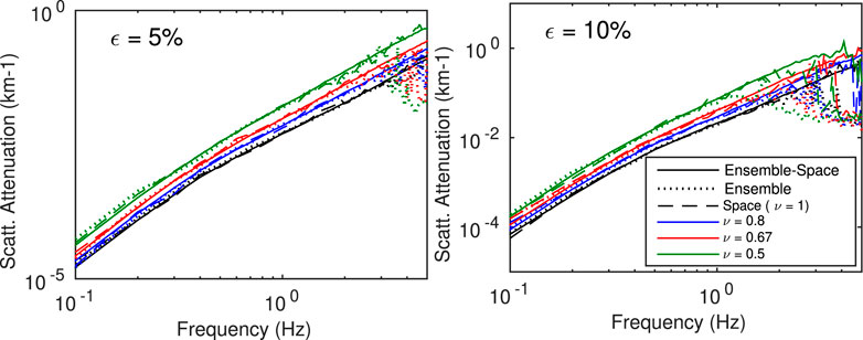
FIGURE 5. Comparison of scattering attenuation estimates obtained with different measures of the coherent wavefield: ensemble average (dotted lines), space average (dashed lines) and ensemble-space Average (solid lines). Left (resp. right) figure corresponds to random media with ε = 5% (resp. ε = 10%).
A comparison between theoretical and numerical scattering estimates is shown in Figure 6. The numerical estimates, referred to as SEM, rely on the ensemble-space average to define the coherent wavefield and the theoretical estimates are obtained by solving (Eq. 7). We retrieve the behaviour illustrated in Figure 1, with an increase of scattering attenuation with frequency like f3 in the low-frequency, Rayleigh regime, and like f2 in the intermediate-frequency, stochastic regime.
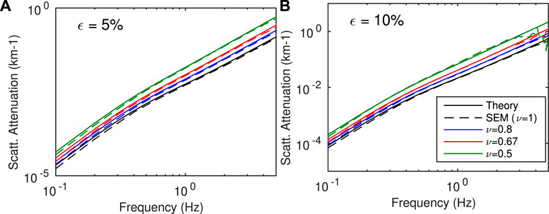
FIGURE 6. Comparison of scattering attenuation between SEM (dashed lines) and the analytical solution (solid lines). SEM solution corresponds to the ensemble-space average approach and the theory is given by the solution of Eq. 7. (A) Cases ε = 5%; (B) Cases ε = 10%.
The results show a very good agreement between SEM estimates and theoretical calculations. As mentioned earlier, some instabilities of the SEM estimates are observed at high frequency for ν = 0.5 and ε = 10%, when the scattering mean free path tends to be comparable or shorter than the minimum inter-station distance. Note also that there is a slight tendency for the SEM estimates to underestimate the theoretical predictions in the Rayleigh regime.
3.2 Comparisons of SEM and RTT intensities
3.2.1 Temporal source term in RTT
The purpose of this section is to clarify our strategy to compare energy envelopes derived from RTT and SEM full wave simulations. We remind the reader that the former theory predicts the ensemble average intensity for quasi-monochromatic waves propagating in a random medium (Ryzhik et al., 1996). In sharp contrast with the wave Eq., RTT operates on quantities that depend quadratically on the wavefield. In seismology, energy envelopes of seismograms are most often defined as the smoothed squared envelope of the analytic signal derived from the observed wavefield ur [e.g. Emoto and Sato (2018)]. Because propagation effects are generally frequency dependent, it is important to localize the observations in the frequency domain by filtering the data prior to envelope computation. Taking this into account, we write:
where G(t) can be understood as the impulse response (Green’s function) of the wave equation, f (t) is a source term (applied force) and ⊗ denotes the convolution product. Note that f incorporates some narrow- band filtering around circular frequency ω0. To alleviate notations, we drop the spatial dependence of field quantities in (Eq. 18) and following. We may now introduce the seismogram energy envelope E(t) as follows:
where ui is the Hilbert transform of ur, u is the (complex) analytic signal derived from ur and the brackets denote an averaging operation. In practice, ensemble averaging is replaced by smoothing in the temporal domain. In the present work, the intensities derived from SEM simulations were averaged over 180 independent realizations of the random medium (60 realizations and three independent receivers Wi, Ci, and Ei, see Section 2.4). To understand the impact of filtering on the energy envelopes derived from RTT, we decompose the intensity over its different frequency components as follows:
where the hat denotes the Fourier transform (FT) of a given function. In (Eq. 20), the pre-factor 4 takes into account the relation between the FT of the real and analytic signals: uˆ(ω) = 2H(ω)uˆr(ω) with H the Heaviside function; the (2π)−2 factor in the integral results from the Fourier transform convention (see for instance Aki and Richards, 2002). For the source term, we ideally think of a function of the form:
where ω0 is the observation frequency and s(t) is an envelope function which varies over a characteristic time T such that ω0T ≫ 1. We also demand that sˆ(ω) converges (up to some pre-factor) to a delta function in the limit T → ∞. As a consequence, we may localize the spectrum of u in an arbitrarily small neighborhood of ω0. Typical examples for s(t) are given by the boxcar function Π(t/T), the half exponential H(t)e−t/T or the Gaussian
The dominant contributions to the integrals come from the intervals |ω − ω0| ≤ B/2, |Ω| ≤ B where B ∝ 1/T is the bandwidth of the envelope s(t). Physically, ω and Ω describe the fast oscillations of the wave and the slow modulation of the seismogram envelope, respectively (Lagendijk and Van Tiggelen, 1996). Note that for all practical purposes, the integration regions may be extended from −∞ to + ∞. If we now assume that the scattering properties vary little inside the frequency band of interest, we may evaluate the ensemble average product of the Green’s function at the central frequency ω0 (or in fact any other convenient frequency within the band). The intensity Green’s functions at the central frequency ω0 may then be defined as:
The solution to the transport (Eq. 10) provides an approximation to I (t, ω0) which, according to (Eq. 22) must be convolved with a source term S(t) whose FT is given by:
By a simple change of variable this is recognized as the auto-correlation of Sˆ(ω) which in turn yields the following approximation for the seismogram envelope in the time domain:
Eq. 25 shows that in the ideal case where the time scale of the envelope is much larger than the period of the waves, the Green’s function of the RTE should be convolved with the squared envelope of the source term of the wave equation. In practice, we rarely reach this perfect separation of scales. For example, the common practice in seismology is to filter the data in a frequency band f0 ± f0/3 with a two-pass Butterworth filter with 4 poles. We also adopt this choice in this work. An additional difficulty stems from the fact that MC simulations average the intensity over a finite volume, in contrast with SEM simulations where intensities are evaluated at a point. To circumvent these difficulties, we therefore identified the source term |s(t)|2 by deconvolving the numerical Green’s functions of RTE from the SEM intensity in a homogeneous medium (see Figure 7). This operation is performed independently for each central frequency of interest at a receiver located 5 kms away from the energy injection surface in the SEM simulations. The deconvolution process and the retrieved source function are depicted in Figure 7. The Green’s function of the RTE in scattering media is then systematically convolved with the identified source term before comparison with the average intensities derived from the SEM simulations. A similar strategy was adopted by Margerin and Nolet (2003) in their modeling of PKP precursors.
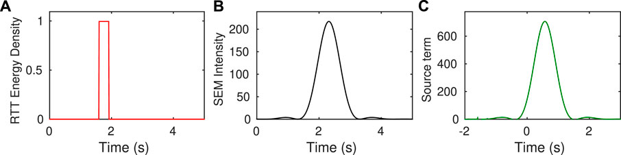
FIGURE 7. Identification of the source term in the radiative transfer equation. At a distance z = 5 km from the source in a non-scattering medium, the energy density predicted by RTT (A) is deconvolved from the intensity computed by SEM simulations (B) to obtain the source time function (C) This example corresponds to the frequency band [1, 2] Hz.
3.2.2 Analysis of RTT and SEM energy envelopes
To examine critically the potential of RTT at modeling the transport of intensity in a random medium, we compare MC simulations of RTT and full wave SEM simulations for a variety of epicentral distances ({50, 100, 150} kms), frequency bands ([0.5, 1] Hz, [1, 2] Hz and [2, 4] Hz), Birch correlation coefficients ({0.5, 0.67, 0.8, 1}) and RMS velocity perturbations ({0.05, 0.1}). The Hurst exponent is fixed at 0.25, which corresponds to random media that are relatively rich in small-scale heterogeneities, thought to be representative of geological materials (Sato, 2019). Referring back to Figures 1, 6, this parametric study allows us to explore a variety of propagation regimes from ballistic/single-scattering (t ≪ τ, with t the lapse-time and τ the scattering mean free time) to diffusive (t ≫ τ) in the Rayleigh and stochastic frequency regions. To facilitate the discussion, we summarize in Table 1 the main characteristics of the random media we considered.
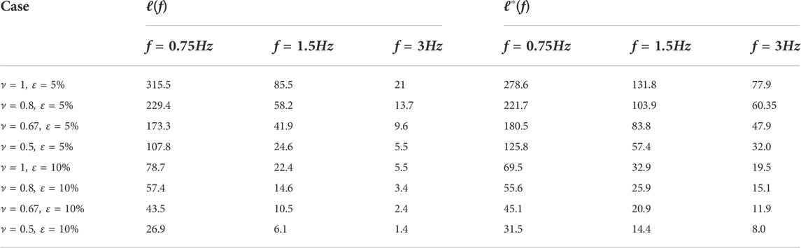
TABLE 1. Scattering (ℓ) and transport (ℓ∗) mean free paths for the set of random media considered in Figures 8, 9. The central frequencies correspond to the analyzed frequency bands ([0.5, 1], [1, 2] and [2, 4] Hz).
Figures 8, 9 show systematic comparisons between SEM and RTT energy envelopes. To suppress statistical fluctuations, the outputs of the full wave simulations have been averaged over 180 realizations.
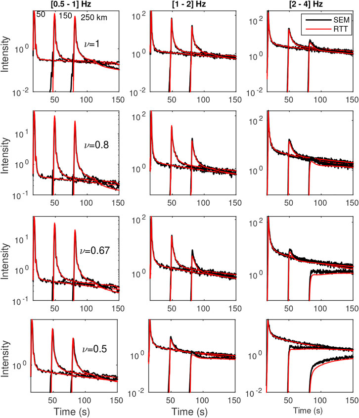
FIGURE 8. Mean intensity comparisons between SEM and radiative transfer theory solution. Results are shown for three frequency bands [0.5 1], [1 2] and [2 4] Hz, and for three different distances, at 50, 150 and 250 km. Red line corresponds to SEM intensities and the black lines are the radiative transfer theory solution. Cases ε = 5%.
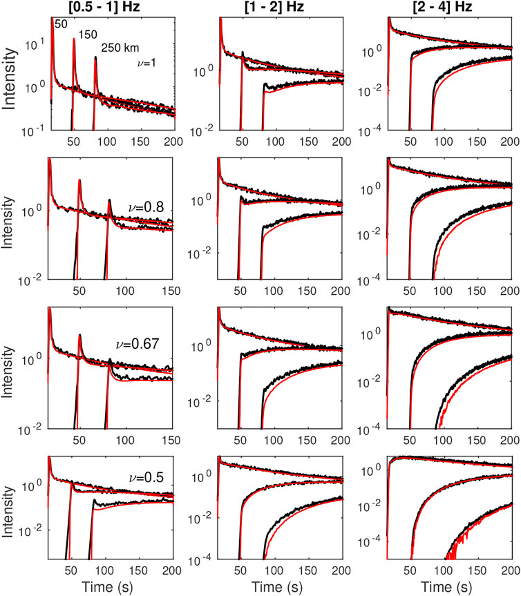
FIGURE 9. Same as Figure 8 for cases ε = 10%.
For the vast majority of cases considered, we find very reasonable agreement between SEM and RTT energy envelopes. This result is quite remarkable considering the fact that the numerical experiments cover almost all propagation regimes that are likely to be met in practice. In the details, we observe that the fit between ab initio simulations and RTT is not uniform in the model parameter space. The worst fits are generally observed for scattering media with small values of ν, large perturbations (ε = 10%), which correspond to increasing strength of scattering. In Figure 9, we find that while RTT reproduces rather well the general envelope shape, it tends to slightly underestimate the amplitude of the ballistic peak and the coda level for the largest propagation distances. The slight discrepancies may find their source in at least three non-trivial differences between the two approaches. First, we may invoke the treatment of BC at the top and bottom of the model. On the one hand, absorbing conditions are perfect in MC simulations of RTT because any seismic phonon that escapes the propagation medium automatically terminates its random walk. In SEM simulations, the implementation of absorbing BC is less efficient [we used the old implementation of Stacey (1988) instead of the PML implementation of Komatitsch and Martin (2007)], so that waves that strike the boundary at large incidence angles get partially reflected, which may in turn explain the largest energy level in the coda. The second source of discrepancy is the finite frequency band used in the simulations. Indeed, scattering attenuation depends strongly on frequency in the Rayleigh regime and slightly less so in the stochastic regime. Hence, it is probably incorrect to assume that the scattering properties are more or less uniform in a given frequency band. In the Rayleigh regime, we did find by direct computations that changing the central frequency from 0.5Hz to 1 Hz (for instance) does increase significantly the level of backscattering in the coda. This may explain the slight underestimation of the coda level for ν = 0.5, 0.67 visible in the low-frequency band for ε = 10%. Our third point is motivated by the observation that the discrepancy between SEM simulations and RTT is amplified as ν decreases and ε increases (compare the left panels in Figures 8, 9). In both cases, this corresponds to an increase in the strength of the scatterers. This therefore suggests that part of the issue stems from the Born approximation which underlies the computation of the scattering properties in RTT. The limitations of Born approximation have been previously noted in the literature, even for scatterers of moderate contrasts (Korneev and Johnson, 1993; Gritto et al., 1995). Additional work will be needed to determine the dominant factor at the origin of difference between RTT and SEM at low frequency.
In the intermediate-to-high frequency regions ([1, 2] Hz, [2, 4] Hz), Figures 8, 9 (middle and right panels) provide illustrations of a variety of classical multiple-scattering phenomena that are remarkably well captured by RTT, as attested with the overall good match with the SEM simulations. This includes the attenuation of the signal, the broadening of the ballistic pulse and the coda generation, which result in a decrease of the coherent to incoherent energy ratio (see for example middle panels in Figure 8). This transfer of energy from the coherent to the incoherent component of the wavefield is in fact the key process described by RTT. The spatio-temporal dependence of the coherent-to-incoherent energy ratio forms the basis for the determination of scattering properties in seismology and acoustics (Fehler et al., 1992; Hoshiba, 1993; De Rosny and Roux, 2001). In the case where the propagation distance of the ballistic wave exceeds the transport mean free path (see in particular the right panels in Figure 9), the energy envelopes develop a shape characteristic of diffusive propagation, with a delay from the onset of the signal to the peak that increases like R2/D with R the hypocentral distance and D the diffusivity of the waves. In Supplementary Figure S2 of the supplementary material, we verify that the diffusion model developed in Section 2.3 provides an excellent match to the SEM envelopes. The overall accuracy and relative simplicity of the diffusion approximation makes it particularly attractive to model the transport of seismic energy through very strongly scattering media such as planetary regoliths (Dainty et al., 1974; Gillet et al., 2017; Karakostas et al., 2021) or volcanoes (Wegler and Lühr, 2001; Wegler, 2003; Del Pezzo, 2008). At sufficiently long lapse-time, we note the progressive homogenization of the spatial distribution of seismic energy, which underpins the so-called coda normalization method (Aki, 1980). Having described in some details the spatio-temporal dependence of the ensemble average intensity in random media, we investigate the intensity fluctuations in the ballistic peak and the coda in the next section.
3.3 Intensity distributions
Although RTT per se does not make predictions on the deviation of the intensity from its mean value, closely related multiple-scattering theories provide some insight on this issue (Rytov et al., 1989). SEM simulations offer a unique opportunity to test the predictions of these theories in some detail. In atmospheric optics, the magnitude of intensity fluctuations as quantified by the scintillation index
It is generally accepted that the statistical distribution of intensity fluctuations differ between the ballistic peak and the coda part. A clear and concise exposition of the basic theory accounting for this difference is provided by Goodman (2015). Here, we shall simply recall the basic distributions that are thought to be representatives of intensity fluctuations around the ballistic peak and in the coda. In the former case, treating the propagation medium as a succession of random phase screens along the direct ray path, perturbation theory yields:
with Fln the cumulative distribution function (CDF) of the Log-normal distribution. In (Eq. 26), µ and σ respectively denote the mean and the standard deviation of the logarithm of intensity. In the case of the coda, the wavefield is thought to be a superposition of many waves with random uncorrelated phases. The central limit theorem then asserts that the field is gaussian, which in turn implies that the intensity (of the derived analytic signal) is exponentially distributed:
To let the reader appreciate the relevance of these distributions to characterize intensity fluctuations in random media, we estimated the empirical CDF of intensity from SEM simulations, as well as the two basic statistics µ and σ. This task was carried out in short time windows of duration 1/fc (fc the central frequency of the filtered data) around two lapse-times T1 and T2 corresponding to the arrival time of the ballistic peak and the late coda (T2 = T1 + 80 s), respectively. 180 realizations of the random medium were employed for the analysis. To investigate different propagation regimes, we compare the empirical CDF with the predictions of the Log-normal and exponential distributions at two different propagation distances (5 kms and 150 kms) from the source. Typical results are shown in Figure 10 at central frequency 1.5 Hz in the case ν = 0.5 and ε = 5%, corresponding to a scattering mean free path ℓ = 24.6 km (see Table 1). At short distance from the source (Figure 10 top), we observe that the Log-normal and exponential distributions provide excellent match to the intensity fluctuations of the ballistic peak and of the coda, respectively. At large distance from the source, the intensity in the coda is unsurprisingly still governed by an exponential distribution. Much more intriguing is the observation that the intensity of the ballistic peak follows an exponential distribution rather than a Log-normal one. The logical explanation for this somewhat paradoxical outcome is that the ballistic peak is composed of multiply-scattered waves. This interpretation is in fact consistent with the value of the scattering mean free path (24.6 km), which implies that the coherent wave has already been almost completely converted to scattered waves at a distance of 150 km from the source. What makes the peak visible is that the single scattering process occurs preferentially around the forward direction. This is attested by the value of the ratio ℓ∗/ℓ (> 2), which is a classical measure of scattering anisotropy (ℓ∗/ℓ > 1 implies dominant forward scattering). The fraction of scattered waves that keeps propagating around the forward direction gives rise to a ‘quasi-ballistic’ peak, whose attenuation properties will be further investigated in Section 3.4.
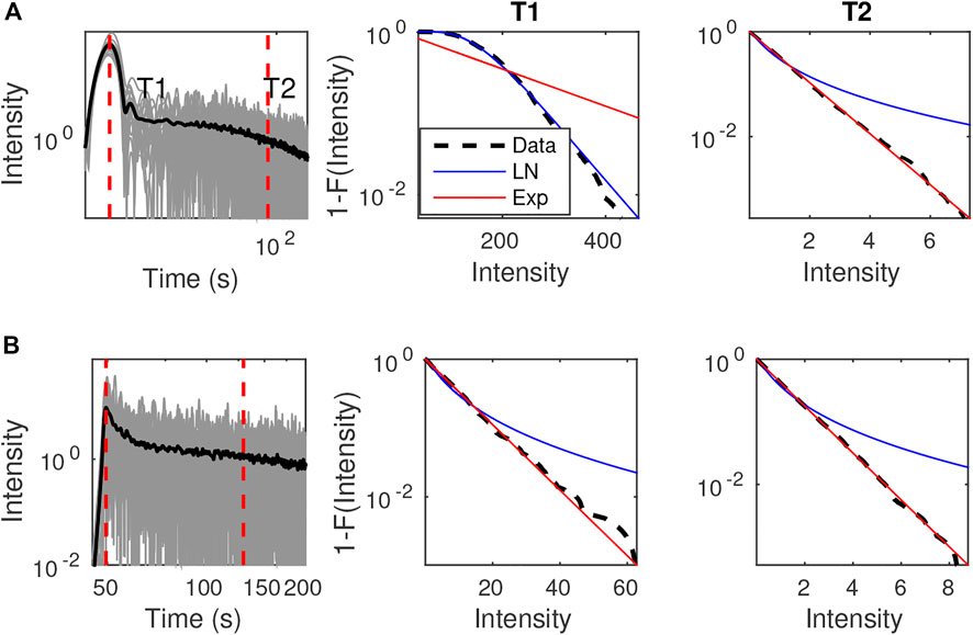
FIGURE 10. Distribution of intensities at distances (A) 5 km and (B) 150 km from the source for the case ν = 0.5, ε = 5% in the [1, 2] Hz frequency band (Left) Ensemble of 180 realizations of SEM intensities (grey lines) and their mean value (black line); (Center and Right): Complement of the CDFs of intensities around lapse times T1 and T2 corresponding to the ballistic peak and the late coda (as indicated by the dashed red lines in the left panels). The solid blue and red lines show the fitted Log-normal and exponential CDF. The black dashed line represents the empirical complementary CDF from SEM simulations.
We will now focus on the intensity distribution of the ballistic peak and its dependence with distance in order to identify the transition from log-normal to exponential behavior. This analysis will give us clues on the crossover between different scattering regimes as the propagation distance z increases: notably from ballistic for z ≤ ℓ to quasi-ballistic for ℓ ≤ z ≤ O (ℓ∗). Emoto and Sato (2018) performed a similar study in the time domain. More precisely, they investigated the lapse-time dependence of the intensity distribution using an ensemble of full waveform simulation in a set of von Kármán media with different statistical parameters. They found that for most cases, the distribution changes from log-normal to exponential just after the ballistic peak. Furthermore, for certain levels of scattering and distance ranges, they could observe the crossover at earlier lapse-times (i.e., in the ballistic peak). Following the procedure of Emoto and Sato (2018), we use the mean absolute error (MAE) to quantify the agreement between the empirical intensity CDF and the predictions of the Log-normal and exponential distributions. Precisely, the MAE is defined as
In Figure 11 we show the distance dependence of MAE of the Log-normal and exponential distributions in three frequency bands ([0.5, 1] Hz, [1, 2] Hz, [2, 4] Hz) in the case ν = 0.8, ε = 5%. Except in the strongest scattering medium (lower right panel), Figure 11 illustrates that the peak intensity distribution is invariably Log-normal at short distance from the source. Conversely, at large distance from the source, we find that the intensity is governed by an exponential probability law, at the exception of the most weakly scattering medium (upper-left panel). Therefore, it is meaningful to track the critical distance Rc at which the transition between the two probability distributions occurs. As outlined previously, this critical distance marks the transition from a ballistic regime where the peak intensity is dominated by the coherent wave to a “quasi-ballistic” regime where the peak is mostly composed of forward-scattered waves. The key idea is to use Rc as a proxy for the scattering mean free path. To test this possibility, we denote by a vertical dashed line the epicentral distance corresponding to the scattering mean free path in Figure. The visual comparison of Rc with ℓ indeed confirms some correlation between the two quantities. In Figure 12, we investigate systematically the dependence of Rc on ℓ for all the cases considered in Table 1. The results clearly suggest that Rc = O(ℓ) and could be used as an upper bound for the scattering mean free path. We are not aware of field observations of the statistical transition seen in SEM simulations.
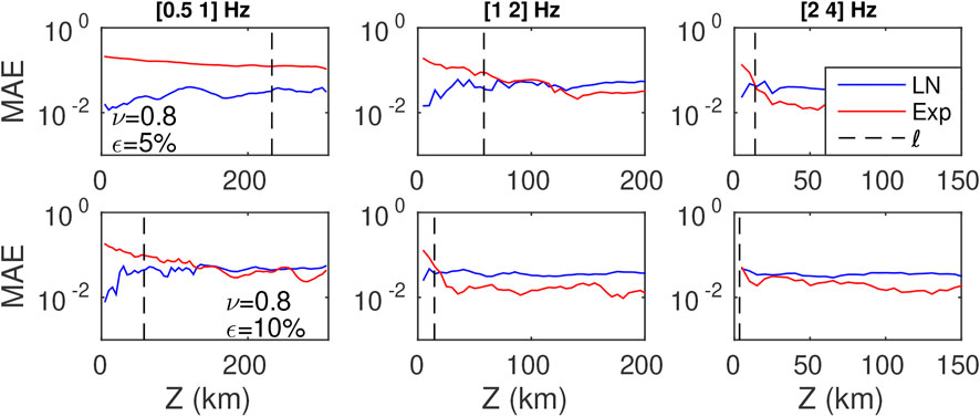
FIGURE 11. Distance dependence of intensity distributions at the ballistic peak for cases ε = 5%. Blue and red lines are the log-normal and exponential distributions, respectively. The dotted black line corresponds to the value of scattering mean free path for each specific central frequency.
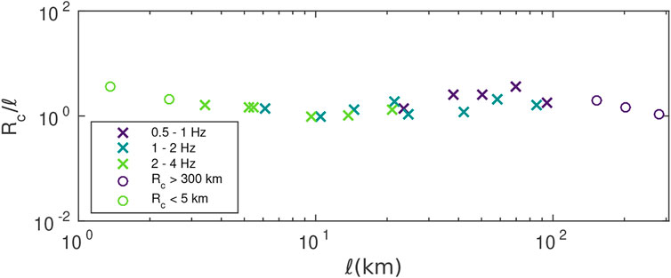
FIGURE 12. Scaled critical distance Rc/ℓ as a function of ℓ. Colors stand for the three frequency bands. The circles denote the cases at which Rc takes values either larger than the maximum epicentral distance (300 km) or shorter than the minimum (5 km).
3.4 Peak intensity attenuation
Since the pioneering works of Wu (1982) and Sato (1982), it is widely accepted that the so-called “direct waves” are in fact a mixture of the coherent and incoherent components of the wavefield. Besides the confounding effect of absorption, the fact that the coherent field is not readily accessible in seismology severely complicates the interpretation of attenuation measurements. The purpose of this section is to shed some light on this issue.
We pointed out in Section 3.3 that for propagation distances typically larger than the mean free path, forward-scattered waves can form a peak of intensity which propagates in a quasi-ballistic fashion. We now investigate specifically the attenuation characteristics of this peak. We first filter the waveforms obtained from SEM simulations in narrow frequency bands 5/6f0, 7/6f0 with f0 increasing from 0.5 Hz to 5 Hz by increment of 0.5 Hz. We used a two-pass Butterworth filter with 4 poles. Intensities are then calculated using the definition (Eq. 19) and averaged over 180 realizations (ensemble average of intensities). The operation is repeated every 5 kms for propagation distances ranging from 5 kms to 300 kms. Finally, at each frequency, we normalize the average intensities by the maximum value sup I (z, t). Normalized peak intensities are displayed as a function of distance for each frequency in Figure 13. Note that since a logarithmic scale is used on the vertical axis, an apparent linear behavior corresponds to an exponential decay in space. Such a behavior is clearly observed at all frequencies at sufficiently short distance from the source. As distance increases the apparent exponential behavior eventually breaks down. This feature is particularly clear for the strongest scattering media for which an abrupt change of the slope can be observed in the peak intensity decay curve. This corresponds to the transition towards the diffusion regime where the maximum intensity is reached in the coda. Similar to Section 3.1, the range of propagation distances for which the intensity decay can be considered exponential was determined by visual inspection resulting in threshold values of intensities ranging from 5% to 10% of the maximum intensity. The apparent attenuation length of the peak intensity (ℓI) is subsequently determined by a simple linear regression of the logarithm of intensity with distance. The results (with respective uncertainties) are shown in Figure 13 (upper right panel). While peak intensity attenuation increases with frequency, comparison with Figure 6 reveals that both its magnitude and frequency dependence differ significantly from the predictions of mean field theory. In other words, the apparent decay length of the peak intensity is not the scattering mean free path.
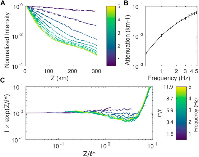
FIGURE 13. Measurement of peak intensity attenuation. (A) Peak intensity decrease with distance (solid lines) and the fitted exponential regression (dashed lines), the colorbar represents different central frequencies ranging from 0.5 to 5 Hz with a frequency step of 0.5 Hz. (B) Peak intensity attenuation and bar errors. (C) dependence of scaled intensity I × exp (z/ℓ∗) versus z/ℓ∗. Case ν = 0.5 ε = 5%.
As discussed in Section 2.3, scattering anisotropy leads to the introduction of the transport mean free path ℓ∗ as a new length scale in RTT. In particular, ℓ∗ appears as the step length of the diffusive process that approximates the solution of the transport problem. It is also the key length scale controlling the broadening of energy envelopes with distance (Gusev and Abubakirov, 1999). Using real data examples, Gaebler et al. (2015) demonstrated that ℓ∗ is so far the only scattering property that can be inferred with some confidence from seismological observations. These facts put forward ℓ∗ as the natural scale length to quantify the peak intensity decay with distance. To put this idea to the test, we plot in Figure 13 (bottom) the normalized intensity rescaled by the factor exp [z/ℓ∗(f)] as a function of z/ℓ∗. Remarkably, we observe at all frequencies that, up to a distance of the order of order ℓ∗, attenuation of the ballistic peak of intensity is very well predicted by the transport mean free path in the case ν = 0.5 and ε = 0.5%. In the case where scattering is weakly anisotropic (i.e., in the lower frequency range), we even find that the exponential decay regime extends beyond 2 transport mean free paths. Note that at low frequency, the scattering and transport mean free path differ in general very little. In this regime, Zhang et al. (1999) found through theoretical and experimental investigations that scattered waves display quasi-ballistic behavior up to a propagation distance of three mean free paths. Although these authors did not investigate the peak attenuation, their findings agree qualitatively with the results shown in Figure 13.
To further document the key role played by ℓ∗ in seismic attenuation, we compare in Figure 14 the peak intensity attenuation ℓ−1 estimated from SEM simulations with the theoretical predictions for ℓ∗−1 and ℓ−1 for the set of random media listed in Table 1. For reference, we also show the attenuation of the peak particle velocity of the coherent wavefield (ensemble-space average), which was previously discussed at length in Section 3.1. Figure 14 provides a solid confirmation that ℓ∗ is indeed a very good approximation to the apparent attenuation length of the peak intensity for a broad range of random media. We recall that the exponential decay of the peak intensity remains valid up to a distance of the order of ℓ∗ with a range of validity which is bit broader when scattering is weakly anisotropic. The Figure also illustrates very clearly that the scattering attenuation length of the mean field and mean intensity differ very largely in the forward scattering regime. This difference is explained by the fact that the mean field represents the pure coherent (unscattered) component, whereas the mean intensity is a mixture of coherent and incoherent (scattered) waves. The waves scattered around the forward direction exhibit a quasi-ballistic behavior with the transport mean free path as the key controlling length scale (Gusev and Abubakirov, 1999).
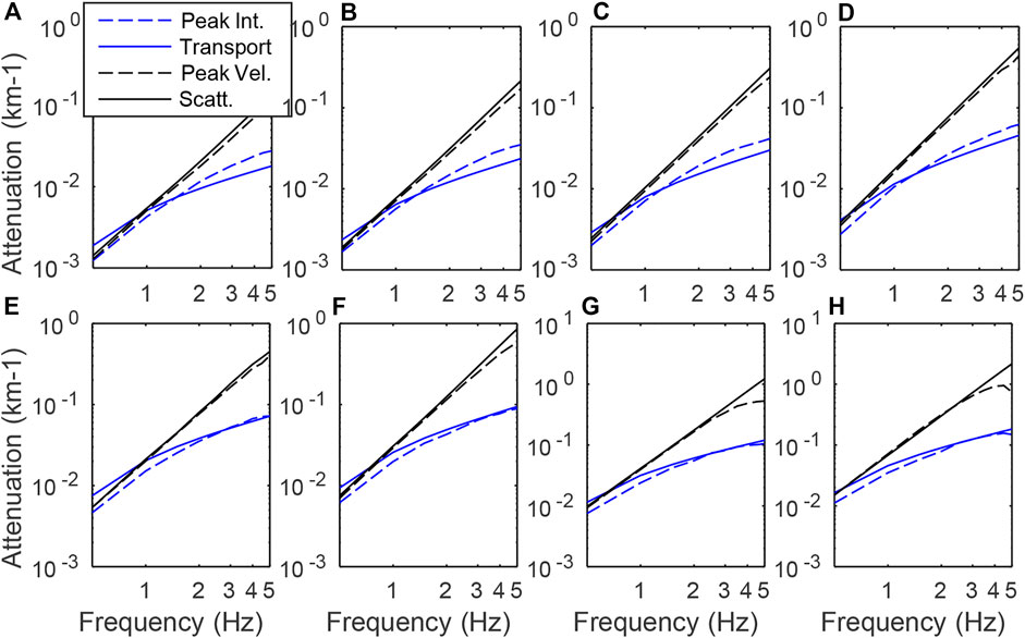
FIGURE 14. Peak intensity attenuation (dashed blue line) and comparison with transport mean free path (solid blue line), peak velocity attenuation of the coherent wave (dashed black line) and scattering mean free path (solid black line). Transport and scattering mean free paths plots correspond to their analytical solutions. Attenuation of the peak intensity is obtained from the ensemble average of the 180 realizations and the peak velocity corresponds to the ensemble-space average coherent wavefield (A–D) cases ε = 5% and (E–H) cases ε = 10%. (A,E) correspond to the case ν = 1, (B,F) to ν = 0.8, (C,G) to ν = 0.67 and (D,H) to ν = 0.5.
4 Conclusion
While it is broadly accepted that small-scale heterogeneities play a key role in realistic simulations of ground motions at high-frequencies, the validation of their implementation remains in our opinion a blind spot. The most comprehensive source of information on small-scale heterogeneities is the inversion of envelope characteristics with the aid of RTT (Abubakirov and Gusev, 1990; Fehler et al., 1992; Hoshiba, 1993; Wang and Shearer, 2017; Sato, 2019). Due to the limited data coverage, this approach offers access to frequency dependent scattering attenuation lengths (the scattering and/or transport mean free paths) but not to the full power spectrum of heterogeneities. Hence, to simulate the correct propagation regime and reproduce reasonably well the characteristics of seismograms, it is important to verify that the mean free path of the numerical model of wave propagation matches the one of the targeted area in the frequency band of interest. With the aid of scattering theories for the mean field and the mean intensities, we have shown in this paper that this task is completely manageable over a broad range of frequencies up to fluctuations of 10% which are typical of the crust. An exception is the very-high frequency limit, which remains challenging both numerically and theoretically (Sato and Emoto, 2018). Full wave simulations also offer access to the statistical distribution of intensity. We payed particular attention to the ballistic peak and found a transition from a log-normal to an exponential distribution at a distance from the source of the order of the scattering mean free path. This implies that in many cases of interest, the ballistic peak is in fact composed of a superposition of multiply-scattered waves, in spite of its “coherent” appearance. This finding has at least two important implications. In seismic hazard assessment, because it is heavy-tailed, the log-normal distribution allows for larger deviations of the intensity from its mean value than the exponential distribution. Having access to the correct propagation regime is therefore important to estimate the typical uncertainty in full wave simulations or in ground motion prediction equations. The full wave simulations also illustrate that the attenuation of the ballistic peak does not follow the attenuation of the coherent wave. While this has been known for a long time (Sato, 1982; Wu, 1982), there have been debates in the literature on the relevant length scale, with several authors advocating the transport mean free path as the key quantity (Gusev and Abubakirov, 1999; Gaebler et al., 2015). Here, we show by direct comparison with full wave simulations that the ballistic peak indeed exhibits an apparent exponential decay with the transport mean free path as attenuation length. We note that this result has been obtained for random media that are richer in small-scale than the usual one with exponential correlation and that further numerical work is needed to investigate the validity of this result for a broader range of Hurst exponents. It nevertheless implies that the basic relation Qsc = ωl/v found in the literature, while theoretically correct, has little relevance to the apparent attenuation seen in typical seismograms.
Data availability statement
The raw data supporting the conclusion of this article will be made available by the authors, without undue reservation.
Author contributions
MC performed the analysis of spectral element synthetics and their comparison to transport theory, participated to the writing of the manuscript. EC performed the spectral element simulations, participated to the analysis of the results and to the writing of the manuscript. LM wrote the codes to compute the predictions of transport theory (RTT and diffusion), participated to the analysis of the spectral element synthetics and to the writing of the manuscript. LS participated to the writing of the manuscript.
Acknowledgments
MC acknowledges financial support from MINCIENCIAS and from the French Colombian ECOS-NORD program. The numerical simulations were performed at the High Performance Computing Center of the Grenoble University on the Dahu cluster of the GRICAD-CIMENT infrastructure (https://gricad.univ-grenoble-alpes.fr).
Conflict of interest
The authors declare that the research was conducted in the absence of any commercial or financial relationships that could be construed as a potential conflict of interest.
Publisher’s note
All claims expressed in this article are solely those of the authors and do not necessarily represent those of their affiliated organizations, or those of the publisher, the editors and the reviewers. Any product that may be evaluated in this article, or claim that may be made by its manufacturer, is not guaranteed or endorsed by the publisher.
Supplementary material
The Supplementary Material for this article can be found online at: https://www.frontiersin.org/articles/10.3389/feart.2022.1033109/full#supplementary-material
References
Abubakirov, I., and Gusev, A. (1990). Estimation of scattering properties of lithosphere of Kamchatka based on Monte-Carlo simulation of record envelope of a near earthquake. Phys. earth Planet. Interiors 64, 52–67. doi:10.1016/0031-9201(90)90005-i
Aki, K. (1980). Attenuation of shear-waves in the lithosphere for frequencies from 0.05 to 25 hz. Phys. Earth Planet. Interiors 21, 50–60. doi:10.1016/0031-9201(80)90019-9
Aki, K., and Richards, P. G. (2002). Quantitative seismology. Sausalito, CA, USA: University Science Books.
Arridge, S. R., and Schotland, J. C. (2009). Optical tomography: Forward and inverse problems. Inverse probl. 25, 123010. doi:10.1088/0266-5611/25/12/123010
Borcea, L., Garnier, J., and Sølna, K. (2021). Onset of energy equipartition among surface and body waves. Proc. R. Soc. A 477, 20200775. doi:10.1098/rspa.2020.0775
Chaljub, E., Komatitsch, D., Vilotte, J.-P., Capdeville, Y., Valette, B., and Festa, G. (2007). “Spectral- element analysis in seismology,” in Advances in wave propagation in heterogenous Earth (Amsterdam, Netherlands: Elsevier), 365–419. doi:10.1016/s0065-2687(06)48007-9
Dainty, A. M., Toksöz, M. N., Anderson, K. R., Pines, P. J., Nakamura, Y., and Latham, G. (1974). Seismic scattering and shallow structure of the moon in oceanus procellarum. Moon 9, 11–29. doi:10.1007/BF00565388
de Hoop, M. V., Garnier, J., and Sølna, K. (2022). System of radiative transfer equations for coupled surface and body waves. Z. Angew. Math. Phys. 73, 177–231. doi:10.1007/s00033-022-01813-w
De Rosny, J., and Roux, P. (2001). Multiple scattering in a reflecting cavity: Application to fish counting in a tank. J. Acoust. Soc. Am. 109, 2431–2597. doi:10.1121/1.4744602
Del Pezzo, E. (2008). Seismic wave scattering in volcanoes. Adv. Geophys. 50, 353–371. doi:10.1016/S0065-2687(08)00013-7
Dolan, S. S., Bean, C. J., and Riollet, B. (1998). The broad-band fractal nature of heterogeneity in the upper crust from petrophysical logs. Geophys. J. Int. 132, 489–507. doi:10.1046/j.1365-246x.1998.00410.x
Emoto, K., and Sato, H. (2018). Statistical characteristics of scattered waves in three-dimensional random media: Comparison of the finite difference simulation and statistical methods. Geophys. J. Int. 215, 585–599. doi:10.1093/gji/ggy298
Fehler, M., Hoshiba, M., Sato, H., and Obara, K. (1992). Separation of scattering and intrinsic attenuation for the Kanto-Tokai region, Japan, using measurements of S-wave energy versus hypocentral distance. Geophys. J. Int. 108, 787–800. doi:10.1111/j.1365-246x.1992.tb03470.x
Frankel, A., and Clayton, R. W. (1986). Finite difference simulations of seismic scattering: Implications for the propagation of short-period seismic waves in the crust and models of crustal heterogeneity. J. Geophys. Res. 91, 6465. doi:10.1029/jb091ib06p06465
Frisch, U. (1968). Probabilistic methods in applied mathematics. New-York: Academic Press, 75–198. chap. Wave propagation in random media.
Gaebler, P. J., Eulenfeld, T., and Wegler, U. (2015). Seismic scattering and absorption parameters in the W- Bohemia/Vogtland region from elastic and acoustic radiative transfer theory. Geophys. J. Int. 203, 1471–1481. doi:10.1093/gji/ggv393
Gillet, K., Margerin, L., Calvet, M., and Monnereau, M. (2017). Scattering attenuation profile of the moon: Implications for shallow moonquakes and the structure of the megaregolith. Phys. Earth Planet. Interiors 262, 28–40. doi:10.1016/j.pepi.2016.11.001
Gritto, R., Korneev, V. A., and Johnson, L. R. (1995). Low-frequency elastic-wave scattering by an inclusion: Limits of applications. Geophys. J. Int. 120, 677–692. doi:10.1111/j.1365-246x.1995.tb01845.x
Gusev, A., and Abubakirov, I. (1999). Vertical profile of effective turbidity reconstructed from broadening of incoherent body-wave pulses—i. General approach and the inversion procedure. Geophys. J. Int. 136, 295–308. doi:10.1046/j.1365-246x.1999.00740.x
Hartzell, S., Harmsen, S., and Frankel, A. (2010). Effects of 3D random correlated velocity perturbations on predicted ground motions. Bull. Seismol. Soc. Am. 100, 1415–1426. doi:10.1785/0120090060
Holliger, K. (1996). Upper-crustal seismic velocity heterogeneity as derived from a variety of P-wave sonic logs. Geophys. J. Int. 125, 813–829. doi:10.1111/j.1365-246x.1996.tb06025.x
Hoshiba, M. (2000). Large fluctuation of wave amplitude produced by small fluctuation of velocity structure. Phys. earth Planet. interiors 120, 201–217. doi:10.1016/s0031-9201(99)00165-x
Hoshiba, M. (1993). Separation of scattering attenuation and intrinsic absorption in Japan using the multiple lapse time window analysis of full seismogram envelope. J. Geophys. Res. 98, 15809–15824. doi:10.1029/93jb00347
Hu, Z., Olsen, K. B., and Day, S. M. (2022). 0–5 Hz deterministic 3-D ground motion simulations for the 2014 La Habra, California, Earthquake. Geophys. J. Int. 230, 2162–2182. doi:10.1093/gji/ggac174
Imperatori, W., and Mai, P. M. (2012). Broad-band near-field ground motion simulations in 3-dimensional scattering media. Geophys. J. Int. 192, 725–744. doi:10.1093/gji/ggs041
Imperatori, W., and Mai, P. M. (2015). The role of topography and lateral velocity heterogeneities on near- source scattering and ground-motion variability. Geophys. J. Int. 202, 2163–2181. doi:10.1093/gji/ggv281
Karakostas, F., Schmerr, N., Maguire, R., Huang, Q., Kim, D., Lekic, V., et al. (2021). Scattering attenuation of the martian interior through coda-wave analysis. Bull. Seismol. Soc. Am. 111, 3035–3054. doi:10.1785/0120210253
Komatitsch, D., and Martin, R. (2007). An unsplit convolutional perfectly matched layer improved at grazing incidence for the seismic wave equation. Geophysics 72, SM155–SM167. doi:10.1190/1.2757586
Komatitsch, D., and Vilotte, J.-P. (1998). The spectral element method: An efficient tool to simulate the seismic response of 2D and 3D geological structures. Bull. Seismol. Soc. Am. 88, 368–392.
Korneev, V. A., and Johnson, L. R. (1993). Scattering of elastic waves by a spherical inclusion—ii. Limitations of asymptotic solutions. Geophys. J. Int. 115, 251–263. doi:10.1111/j.1365-246x.1993.tb05602.x
Kourganoff, V. (1969). Introduction to the general theory of particle transfer. Boca Raton, FL, USA: CRC Press.
Lagendijk, A., and Van Tiggelen, B. A. (1996). Resonant multiple scattering of light. Phys. Rep. 270, 143–215. doi:10.1016/0370-1573(95)00065-8
Lux, I., and Koblinger, L. (2018). Monte Carlo particle transport methods: Neutron and photon calculations. Boca Raton, FL, USA: CRC Press.
Margerin, L., Bajaras, A., and Campillo, M. (2019). A scalar radiative transfer model including the coupling between surface and body waves. Geophys. J. Int. 219, 1092–1108. doi:10.1093/gji/ggz348
Margerin, L. (2005). “Introduction to radiative transfer of seismic waves,” in Seismic Earth: Array analysis of broadband seismograms (Washington, DC, USA: American Geophysical Union), 229–252. doi:10.1029/157gm14
Margerin, L., and Nolet, G. (2003). Multiple scattering of high-frequency seismic waves in the deep Earth: PKP precursor analysis and inversion for mantle granularity. J. Geophys. Res. 108, 2514. doi:10.1029/2003jb002455
Müller, T., and Shapiro, S. (2003). Amplitude fluctuations due to diffraction and refraction in anisotropic random media: Implications for seismic scattering attenuation estimates. Geophys. J. Int. 155, 139–148. doi:10.1046/j.1365-246x.2003.02020.x
Nakahara, H., and Carcolé, E. (2010). Maximum-likelihood method for estimating coda Q and the Nakagami-m parameter. Bull. Seismol. Soc. Am. 100, 3174–3182. doi:10.1785/0120100030
Paasschens, J. (1997). Solution of the time-dependent Boltzmann equation. Phys. Rev. E 56, 1135–1141. doi:10.1103/physreve.56.1135
Przybilla, J., and Korn, M. (2008). Monte Carlo simulation of radiative energy transfer in continuous elastic random media—Three-component envelopes and numerical validation. Geophys. J. Int. 173, 566–576. doi:10.1111/j.1365-246x.2008.03747.x
Przybilla, J., Korn, M., and Wegler, U. (2006). Radiative transfer of elastic waves versus finite difference simulations in two-dimensional random media. J. Geophys. Res. 111, B04305. doi:10.1029/2005jb003952
Rudnick, J., and Gaspari, G. (2004). Elements of the random walk: An introduction for advanced students and researchers. Cambridge, UK: Cambridge University Press.
Rytov, S. M., Kravcov, Y. A., and Tatarskij, V. I. (1989). Wave propagation through random media. Berlin, Germany: Springer.
Ryzhik, L., Papanicolaou, G., and Keller, J. B. (1996). Transport equations for elastic and other waves in random media. Wave motion 24, 327–370. doi:10.1016/s0165-2125(96)00021-2
Sanborn, C. J., Cormier, V. F., and Fitzpatrick, M. (2017). Combined effects of deterministic and statistical structure on high-frequency regional seismograms. Geophys. J. Int. 210, 1143–1159. doi:10.1093/gji/ggx219
Sato, H. (1982). Amplitude attenuation of impulsive waves in random media based on travel time corrected mean wave formalism. J. Acoust. Soc. Am. 71, 559–564. doi:10.1121/1.387525
Sato, H. (1984). Attenuation and envelope formation of three-component seismograms of small local earthquakes in randomly inhomogeneous lithosphere. J. Geophys. Res. 89, 1221–1241. doi:10.1029/jb089ib02p01221
Sato, H., and Emoto, K. (2018). Synthesis of a scalar wavelet intensity propagating through von Kármán-type random media: Radiative transfer theory using the born and phase-screen approximations. Geophys. J. Int. 215, 909–923. doi:10.1093/gji/ggy319
Sato, H., Fehler, M. C., and Maeda, T. (2012). Seismic wave propagation and scattering in the heterogeneous earth. Berlin, Germany: Springer Science & Business Media.
Sato, H. (1994). Formulation of the multiple non-isotropic scattering process in 2-D space on the basis of energy-transport theory. Geophys. J. Int. 117, 727–732. doi:10.1111/j.1365-246x.1994.tb02465.x
Sato, H. (2019). Power spectra of random heterogeneities in the solid Earth. Solid earth. 10, 275–292. doi:10.5194/se-10-275-2019
Savran, W., and Olsen, K. (2019). Ground motion simulation and validation of the 2008 Chino Hills earthquake in scattering media. Geophys. J. Int. 219, 1836–1850. doi:10.1093/gji/ggz399
Scalise, M., Pitarka, A., Louie, J. N., and Smith, K. D. (2021). Effect of random 3D correlated velocity perturbations on numerical modeling of ground motion from the Source Physics Experiment. Bull. Seismol. Soc. Am. 111, 139–156. doi:10.1785/0120200160
Shapiro, S. A., and Kneib, G. (1993). Seismic attenuation by scattering: Theory and numerical results. Geophys. J. Int. 114, 373–391. doi:10.1111/j.1365-246x.1993.tb03925.x
Shearer, P. M., and Earle, P. S. (2004). The global short-period wavefield modelled with a Monte Carlo seismic phonon method. Geophys. J. Int. 158, 1103–1117. doi:10.1111/j.1365-246x.2004.02378.x
Shiomi, K., Sato, H., and Ohtake, M. (1997). Broad-band power-law spectra of well-log data in Japan. Geophys. J. Int. 130, 57–64. doi:10.1111/j.1365-246x.1997.tb00987.x
Stacey, R. (1988). Improved transparent boundary formulations for the elastic-wave equation. Bull. Seismol. Soc. Am. 78, 2089–2097. doi:10.1785/BSSA0780062089
Stakgold, I., and Holst, M. J. (2011). Green’s functions and boundary value problems. Hoboken, NJ, USA: John Wiley & Sons.
Stanke, F. E., and Kino, G. S. (1984). A unified theory for elastic wave propagation in polycrystalline materials. J. Acoust. Soc. Am. 75, 665–681. doi:10.1121/1.390577
Takemura, S., Furumura, T., and Maeda, T. (2015). Scattering of high-frequency seismic waves caused by irregular surface topography and small-scale velocity inhomogeneity. Geophys. J. Int. 201, 459–474. doi:10.1093/gji/ggv038
Tchawe, F. N., Gelis, C., Bonilla, L. F., and Lopez-Caballero, F. (2021). Effects of 2-D random velocity perturbations on 2-D SH short-period ground motion simulations in the basin of Nice, France. Geophys. J. Int. 226, 847–861. doi:10.1093/gji/ggab141
Tregoures, N. P., and Van Tiggelen, B. A. (2002). Quasi-two-dimensional transfer of elastic waves. Phys. Rev. E 66, 036601. doi:10.1103/physreve.66.036601
Turner, J. A., and Weaver, R. L. (1994). Radiative transfer and multiple scattering of diffuse ultrasound in polycrystalline media. J. Acoust. Soc. Am. 96, 3675–3683. doi:10.1121/1.410587
van Driel, M., Ceylan, S., Clinton, J. F., Giardini, D., Horleston, A., Margerin, L., et al. (2021). High-frequency seismic events on Mars observed by InSight. J. Geophys. Res. Planets 126, e2020JE006670. doi:10.1029/2020je006670
Wang, W., and Shearer, P. (2017). Using direct and coda wave envelopes to resolve the scattering and intrinsic attenuation structure of Southern California. J. Geophys. Res. Solid Earth 122, 7236–7251. doi:10.1002/2016jb013810
Weaver, R. L. (1990). Diffusivity of ultrasound in polycrystals. J. Mech. Phys. Solids 38, 55–86. doi:10.1016/0022-5096(90)90021-u
Wegler, U. (2003). Analysis of multiple scattering at Vesuvius volcano, Italy, using data of the TomoVes active seismic experiment. J. Volcanol. Geotherm. Res. 128, 45–63. doi:10.1016/s0377-0273(03)00246-4
Wegler, U., Korn, M., and Przybilla, J. (2006). Modeling full seismogram envelopes using radiative transfer theory with born scattering coefficients. Pure Appl. Geophys. 163, 503–531. doi:10.1007/s00024-005-0027-5
Wegler, U., and Lühr, B. G. (2001). Scattering behaviour at Merapi volcano (Java) revealed from an active seismic experiment. Geophys. J. Int. 145, 579–592. doi:10.1046/j.1365-246x.2001.01390.x
Wu, R.-S. (1982). Mean field attenuation and amplitude attenuation due to wave scattering. Wave motion 4, 305–316. doi:10.1016/0165-2125(82)90026-9
Wu, R.-S. (1985). Multiple scattering and energy transfer of seismic waves – separation of scattering effect from intrinsic attenuation – i. theoretical modelling. Geophys. J. Int. 82, 57–80. doi:10.1111/j.1365-246x.1985.tb05128.x
Wu, R.-S., Xu, Z., and Li, X.-P. (1994). Heterogeneity spectrum and scale-anisotropy in the upper crust revealed by the German Continental Deep-Drilling (KTB) Holes. Geophys. Res. Lett. 21, 911–914. doi:10.1029/94gl00772
Xu, Z., Margerin, L., and Mikesell, T. D. (2022). Monte Carlo simulations of coupled body-and Rayleigh-wave multiple scattering in elastic media. Geophys. J. Int. 228, 1213–1236. doi:10.1093/gji/ggab370
Yang, L., Lobkis, O., and Rokhlin, S. (2011). Shape effect of elongated grains on ultrasonic attenuation in polycrystalline materials. Ultrasonics 51, 697–708. doi:10.1016/j.ultras.2011.02.002
Yoshimoto, K., Takemura, S., and Kobayashi, M. (2015). Application of scattering theory to p-wave amplitude fluctuations in the crust. Earth Planets Space 67, 199. doi:10.1186/s40623-015-0366-0
Zeng, Y. (1993). Theory of scattered P-and S-wave energy in a random isotropic scattering medium. Bull. Seismol. Soc. Am. 83, 1264–1276. doi:10.1785/bssa0830041264
Zhang, Z. Q., Jones, I. P., Schriemer, H. P., Page, J. H., Weitz, D. A., and Sheng, P. (1999). Wave transport in random media: The ballistic to diffusive transition. Phys. Rev. E 60, 4843–4850. doi:10.1103/physreve.60.4843
Keywords: numerical simulation, random media, scattering, coherent wavefield, scattering attenuation, transport scattering attenuation
Citation: Celorio M, Chaljub E, Margerin L and Stehly L (2022) Propagation of 2-D SH waves in random media: Insights from ab initio numerical simulations and transport theory. Front. Earth Sci. 10:1033109. doi: 10.3389/feart.2022.1033109
Received: 31 August 2022; Accepted: 02 November 2022;
Published: 28 November 2022.
Edited by:
Paul Cupillard, Université de Lorraine, FranceReviewed by:
Francisco Sanchez-Sesma, National Autonomous University of Mexico, MexicoRégis Cottereau, UPR7051 Laboratoire de mécanique et d’acoustique (LMA), France
Copyright © 2022 Celorio, Chaljub, Margerin and Stehly. This is an open-access article distributed under the terms of the Creative Commons Attribution License (CC BY). The use, distribution or reproduction in other forums is permitted, provided the original author(s) and the copyright owner(s) are credited and that the original publication in this journal is cited, in accordance with accepted academic practice. No use, distribution or reproduction is permitted which does not comply with these terms.
*Correspondence: Emmanuel Chaljub, ZW1tYW51ZWwuY2hhbGp1YkB1bml2LWdyZW5vYmxlLWFscGVzLmZy