
94% of researchers rate our articles as excellent or good
Learn more about the work of our research integrity team to safeguard the quality of each article we publish.
Find out more
METHODS article
Front. Earth Sci. , 11 January 2023
Sec. Solid Earth Geophysics
Volume 10 - 2022 | https://doi.org/10.3389/feart.2022.1030326
This article is part of the Research Topic Applications of Machine Learning in Seismology View all 7 articles
 Yiran Jiang1
 Jingchong Wen1Yuan Tian1Mengyu Wu2Jieyuan Ning1,3,4*
 Yongxiang Shi1Han Wu1Tong Zhou5Jiaqi Li6Tiezhao Bao1
Surface wave is an energy-rich component of the seismic wavefield and has been widely employed in understanding underground structures due to its dispersive nature. One key work in improving the accuracy of dispersion curve measurement is selecting proper cycles and valid frequency ranges. Although manual selection could provide high-quality results, it is hardly possible to handle the explosive growth of seismic data. Conventional automatic approaches with the ability to handle massive datasets by their statistical features require prior assumptions and choices of parameters. However, these operations could not keep away from biases in empirical parameters and thus could not assure high-quality outputs, which might deteriorate the resolution of seismic inversion. To make good use of the waveform information, we develop a deep-learning-based neural network called ‘Surf-Net’. It extracts and selects the surface-wave dispersion curves directly from the waveform cross-correlations (CC) and distance information rather than from frequency-time transformed images or pre-extracted dispersion curves. Taking the velocity measurement task as an arrival time picking problem, Surf-Net is designed to output multiple-channel probability distributions in the time domain for target frequencies, which peak at the arrival times of valid frequencies and remain close to zero elsewhere. We train and test Surf-Net using observational data manually obtained from seismograms recorded by a regional network in Northeast China and synthetic data based on a global seismic velocity model. By comparing Surf-Net with the conventional method in both dispersion curves and inversion results, we show Surf-Net’s remarkable performance, robustness and potential for providing high-quality dispersion curves from massive datasets, especially in low frequencies.
The dispersion curves of seismic surface waves can be utilized to invert for the velocity structure from few meters to hundreds of kilometers in depth (e.g., Zielhuis and Nolet, 1994; Trampert and Woodhouse, 1996; Xia et al., 1999; Shapiro and Ritzwoller, 2002). To avoid the difficulty in determining initial phases, there are generally two primary strategies for the extraction of dispersion curves based on either two-station approaches (e.g., Sato, 1955; Knopoff, 1972; Kovach, 1978) or multichannel ones (e.g., Park et al., 1999, 2007; Xia et al., 1999; Li and Chen, 2020). Unlike the multichannel strategies, the two-station-based methods do not need dense station distributions and are thus widely used in situations with large inter-station distances. However, this kind of methods often has difficulty in phase cycle selection and is more easily affected by noise and needs manual (e.g., Meier et al., 2004; Tian et al., 2017) or automatic selections (e.g., Yao et al., 2006; Bensen et al., 2007) from pre-extracted dispersion curves for improving accuracy.
The manual selection methods provide high-quality dispersion curves but are more costly, making it difficult to handle the massively increasing amount of seismic data. The conventional automatic techniques often rely on criteria such as the velocity range, dispersion curve’s smoothness, and wavefront smoothness (e.g., Yao et al., 2006; Bensen et al., 2007; Lin et al., 2009), which are dependent upon assumptions including the quality of the reference model, velocity-structure smoothness, and weak horizontal inhomogeneity. Besides, the parameters must be carefully determined with few objective standards, while the selection quality is not always guaranteed. As the accuracy of dispersion curves directly influences the quality of the velocity inversion, developing methods to handle the dispersion curve selection both precisely and efficiently is crucial.
The recent development of deep learning theories and methods provides efficient ways of learning complex features from labeled samples. There are many attempts to apply them to seismic data processing, many of which achieve promising results (e.g., Jia and Ma, 2017; Zhao et al., 2019; Zhou et al., 2019; Zhu and Beroza, 2019; Liu et al., 2020). At the same time, past efforts have accumulated numerous manually-selected dispersion curves which can be used as the needed labeled data. The well-developed deep-learning methods and massive amounts of accumulated data make it possible to develop effective high-dimensional criteria for extracting higher-quality dispersion curves.
The applications of deep-learning methods in surface-wave dispersion curve extraction mostly pick from images obtained by frequency-time analysis procedures (Zhang et al., 2020; Dai et al., 2021; Dong et al., 2021; Yang et al., 2022). As both the time-frequency analysis and dispersion curve pre-extraction are not always robust, we would like to use the original waveforms instead, hoping that the deep-learning methods can learn a robust way to extract dispersion curves. We thus develop a deep-learning-based method called “Surf-Net” to extract and select dispersion curves directly from waveform cross-correlations (CCs) and distance information. Taking the extraction problem as a multiple arrival-time-picking task, Surf-Net is trained to output the multiple-channel probability distributions along the time axis, which peak at the arrival times for valid frequencies and remain zeros elsewhere.
We focus on the Rayleigh-wave phase-velocity dispersion curves for clarity and simplicity, while its frame can be used for other problems like Love surface-wave and group-velocity dispersion curves. We train and test Surf-Net via high-quality manually-selected Rayleigh-wave phase-velocity dispersion curves from earthquakes recorded by stations in Northeast China and synthetic data based on a global velocity model. To illustrate Surf-Net’s performance and robustness, we compare it with manual and conventional automatic methods, and apply its extraction results to tomography inversions.
A sufficient number of high-quality dispersion curves are necessary for training deep-learning models. Our dataset consists of observational data with manually-selected dispersion curves and synthetic data. Dispersion curves from a single earthquake and those averaged over a group of curves are respectively referred to as “single” and “average” dispersion curves. The extraction of velocity on a dispersion curve at a specific frequency is referred to as a “pick”.
Using the two-station method (Meier et al., 2004) based on the multiple-filter technique (MFT: Dziewonski and Hales, 1972) and manual selection, Tian et al. (2017) obtained 1,088 inter-station high quality path-averaged dispersion curves of fundamental Rayleigh-wave from 68,642 dispersion curves using 1,463 earthquakes recorded by 49 stations in Northeast China (Figure 1). We use these waveforms and their extracted dispersion curves as the labelled observational data. Considering their specific distribution of inter-station distances and frequencies, we focus on station pairs with inter-station distances D ∈ [120 km, 1800 km] and picks with frequencies f ∈ [1/120 Hz, 1/10 Hz] to make sure the focused data space is covered with enough samples. We set 50 target frequencies decreasing exponentially from 1/10 Hz to 1/120 Hz. For selected curves, the angles between two great circles, one connecting the two stations in a station pair and the other connecting the nearest station and the event, must be smaller than 10°. At the same time, their corresponding signal-to-noise ratios of earthquake waveforms must be larger than 3.

FIGURE 1. (A) A global map showing the distributions of earthquakes (black dots) and stations (blue triangles) used in Tian et al. (2017). (B) A regional map of Northeast China with triangles showing the stations’ distribution, and the red ones are the stations taken as examples below.
We re-check these dispersion curves using themselves as reference velocities and discard picks with differences larger than 5%. The single curves with more than 15% discarded picks and average picks with standard deviations larger than 1.5% are also removed. Considering heavily noise-affected picks would introduce biases into the average results, we remove picks with differences from the average value larger than 2%. The station pairs with average curves covering fewer than 30% target frequencies are removed too.
The original earthquake waveforms are bandpass filtered between 1/140 Hz and 1/8 Hz by a zero-phase filter. Two half-Gaussian functions taper the waveforms near the two ends of the time window [Δ/vmax, Δ/vmin] to retain primary surface waves with velocities in the range [vmin, vmax], where Δ is the epicentral distance. vmin and vmax are set to 1.5 km/s and 6 km/s, respectively. The cross-correlation waveforms are calculated from the processed waveforms recorded by different stations and then filtered by a zero-phase bandpass filter between 1/140 Hz and 1/8 Hz.
To divide the station pairs into training, validation and test sets, we use stratified sampling based on inter-station distances. The training, validation, and test sets have 510, 64 and 64 unique station pairs with 19,499, 2438, and 2181 single dispersion curves, respectively (Figures 2A–F). To expand datasets with narrow distributions (Figures 2A–F), we propose two ways to generate new data from the original ones by shifting the waveforms and changing the input inter-station distance D (Supplementary Information S1). The expanded observational datasets are distributed in broader ranges (Figures 2G–I).
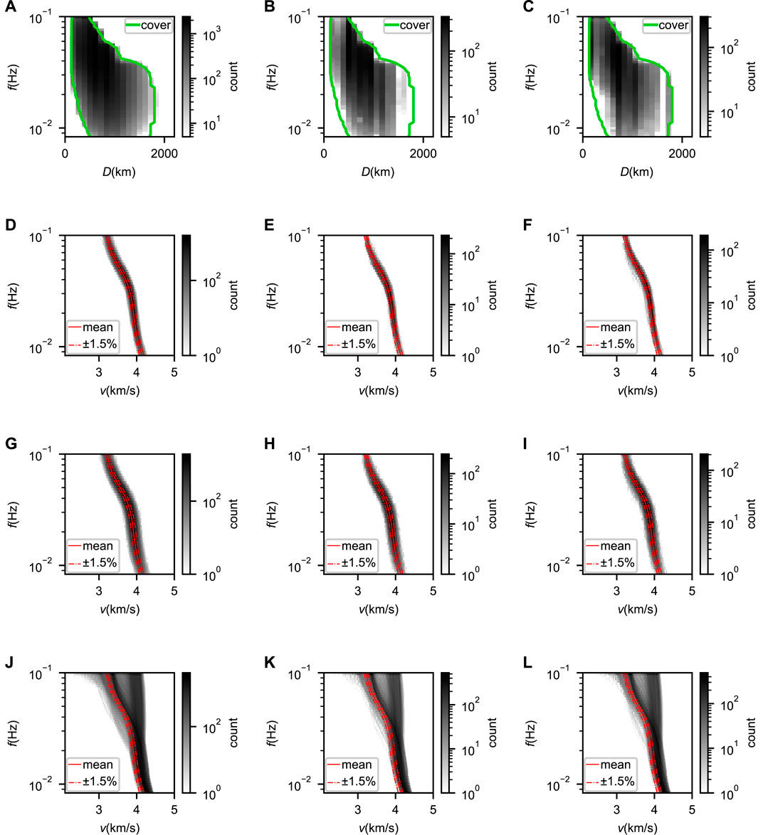
FIGURE 2. (A) Frequency vs. distance distribution of single dispersion curves from the training set plotted in grayscale. The green lines indicate the minimum and maximum distances for different frequencies. (B) and (C) Same as (A) but for the validation and test sets, respectively. (D) Frequency vs. velocity distribution of single dispersion curves from the training set plotted in grayscale. The average of all single dispersion curves is shown as by the solid red line with ±1.5% variation indicated by the red dash lines. (E) and (F) Same as (D) but for the validation and test sets, respectively. (G–I) Same as (D–F) but for the expanded datasets. (J–L) Same as (D–F) but for the synthetic data.
To further expand the coverage of the datasets, we generate synthetic cross-correlation waveforms based on 64,800 dispersion curves. These dispersion curves correspond to 1D velocity models sampled from a seismic velocity model (Lei et al., 2020) with a 1° × 1° interval. Using stratified sampling based on sampling locations, we divide the dispersion curves into the training, validation, and test sets with amounts of 51840, 6480 and 6480, respectively. Their frequency vs. velocity distributions are shown in Figures 2J–L. For a specific dispersion curve, the synthetic waveform cross-correlations are calculated by stacking a series of harmonic waveforms with different frequencies fj:
where, ωj (= 2πfj) indicates the jth harmonic waveform’s angular frequency, kj (= ωj/v (fj)) represents the wavenumber, and Aj is the amplitude. v (fj) is the phase velocity at frequency fj. D is randomly set in the [120km, 1800 km] range. The final synthetic CC is added with noise by
where, the shifted signal R ⋅ c (t + dt, D) is used to simulate interference from other wave packets and random signal n(t) is used as the random noise. dt is a random time shift whose absolute value is larger than 1.5 times the maximum valid period. R is a random amplitude ratio of the shifted signal to the original signal, whose absolute values are smaller 15%. For n(t), its energy at each frequency is smaller than 10% of the original signal, and the phases are set randomly.
On the one hand, the short travel times for station pairs with small inter-station distances lead to non-negligible measurement error at long periods (Yao et al., 2006). On the other hand, for pairs with large inter-station distances and therefore large travel times, the corresponding velocity difference between two adjacent short-period cycles is too small to be selected properly. For a station pair with a certain inter-station distance, we limit pick’s period to the range of
As shown in Figures 2A–C by green lines, the coverage of the inter-station distances can be described by Dmax(f) and Dmin(f), which respectively mean the maximum and minimum inter-station distances for a specific frequency f. To avoid decreases in accuracy, we would remove predicted picks with inter-station distances outside the range of [Dmin(f), Dmax(f)].
The training, validation and test sets finally consist of both synthetic and observational data. We use the training set to train the neural network until the neural network’s performance deteriorates on the validation set and then evaluate the neural network’s final performance via the test set.
Taking the extracting-and-selecting problem for surface-wave dispersion curves as a multiple-arrival-time determination task, we construct both inputs and target outputs in the time domain and build a deep-learning network to find the mapping relationship between them. We now introduce the construction of inputs and target outputs, the structure of the neural network, and necessary outlier removal.
The input contains the CC and distance channel, corresponding to the waveform cross-correlations and distance information. According to our datasets’ range of inter-station distances and the corresponding travel times, the two channels are designed to start from -384 s and last for 1536 s with a 2 Hz sampling rate, containing 3,072 sampling points. The CC channel consists of the cross-correlation waveform and is normalized by the maximum absolute values.
In the distance channel, the inter-station distances are converted into the time domain by a boxcar function:
where the two reference velocities v0 and v1 are 1.5 km/s and 5 km/s, respectively. The values are one if the times t ∈ [D/v0, D/v1] and zero otherwise. The two reference velocities are determined according to the primary velocity range of Rayleigh waves at the target frequencies.
The output is a 50-channel time series corresponding to the 50 target frequencies, representing the probability distributions of surface-wave arrivals, which peak at the arrival times of valid frequencies and remain close to zero elsewhere. At a specific frequency f, the shape of the probability distribution is a Gaussian function with a standard deviation σ(f) varying with the SD (standard deviation) of arrival time measurement errors. The measurement errors of labeled data were evaluated with the final average dispersion curves as the ground truth. As shown in Figure 3A, the SD distribution along the frequency can be approximately fitted by a logarithmic function as
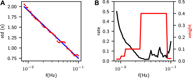
FIGURE 3. (A) The standard deviation (red dots) of single-pick errors at target frequencies and the logarithmic function for approximation (blue line). (B) The rate of dropped picks of the observational data at target frequencies (black line) and the corresponding weights for corresponding dropped channels (red line).
and we set σ(f) equal to this function.
Figure 4 shows six examples of inputs with their target outputs from the test set, which include four observational, one synthetic and one noise examples with different inter-station distances.
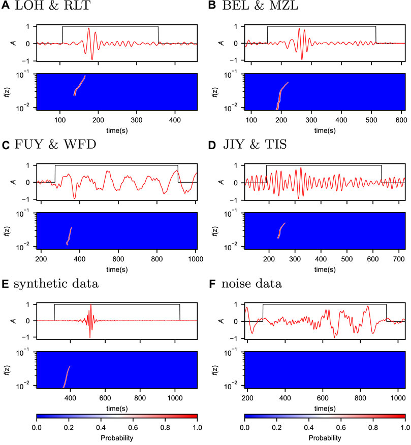
FIGURE 4. Six examples of inputs with their target outputs from the test set, four observational data (A–D), one synthetic data (E) and one of noise (F). The top panel in each example shows the inputs, where the red and black lines represent the CC and distance channels, respectively, and the bottom panel in each example represents the target outputs. To emphasize the primary information, we adjusted the range of shown time windows according to the corresponding inter-station distances.
Surf-Net is an end-to-end neural network modified from the U-net (Ronneberger et al., 2015), which outputs a 50-channel time series with the same length as the input (Figure 5). It has one large-kernel convolution unit, six down-sampling units, six up-sampling units, six skipping connections, and one output unit.
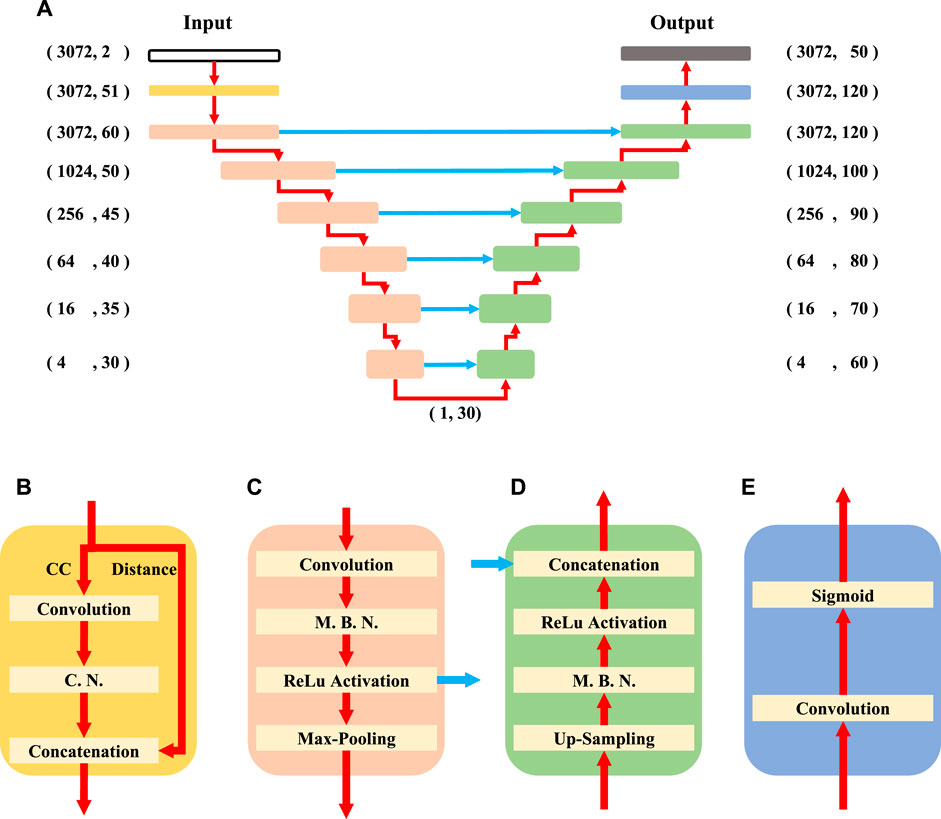
FIGURE 5. The structure of Surf-Net (A) and the large-kernel convolution (B), down-sampling (C), up-sampling (D) and output (E) units. The red arrows present the data flow, and the blue ones are skipping connections. In (A), the (n, m) combination next to a specific unit shows the data flow shape, where n and m are the numbers of sampling points and channels, respectively. In (B), the input data flow is first divided into the CC and distance channels. The convolution and channel normalization layers are then sequentially applied to the CC channel. The two divided flows are finally concatenated together. The C. N. and M. B. N. are short for the channel normalization layer and momentum batch normalization layer, respectively. All the convolution layers are depthwise separable.
To reduce the number of parameters while keeping almost equal fitting ability, we use the depthwise separable convolution instead of the traditional convolution (Chollet, 2017). It decomposes the traditional convolution operation into two steps, the first convoluting along the time dimension of each feature channel and the next projecting the obtained features of each sampling point into new features, which reduces the parameter size by a factor of the channel number.
As the input and output sizes of each sample in our training are respectively large, we can only set a small batch size. So using the original batch normalization layer would result in heavy mini-batch dependency (Ioffe, 2017). Instead of directly using the mean and variance of the current mini-batch, the momentum batch normalization layer (Yong et al., 2020) evaluates the mean and variance with the current and historical mini-batches together and can thus provide better performance with a small batch size. So, we use the momentum batch normalization layer in our network.
The large-kernel convolution unit (Figure 5B) is used to extract features of long periods, which is crucial for processing surface waveforms with long periods. In this unit, the convolution layer with a large kernel applied to the CC channel is designed to obtain a large effective receptive field (Ding et al., 2022). Its kernel size is 960, corresponding to a time window of 480 s, which is four times the maximum focused period. As the major deep learning framework has not fully optimized the time-domain large-kernel convolution operations, we perform the large-kernel convolution in the frequency domain to reduce the time cost. The needed fast Fourier transform operation and its back-propagation have already been natively supported by mainstream deep learning frameworks. This layer would expand the one CC channel into 50 feature channels. The surface wave’s energy at different frequencies varies significantly, causing some difficulty in extraction. To avoid this, we add the channel normalization layer to normalize each channel independently by its maximum value, similar to the instance normalization (Ulyanov et al., 2016). The 50 normalized feature channels are then concatenated with the distance channel by the concatenation layer.
The down-sampling units (Figure 5C) are used to extract features and shorten the data length for higher-level feature extraction. In each down-sampling unit, the convolution layer is followed by a momentum batch normalization layer, an activation layer of the rectified linear unit (ReLU) (Glorot et al., 2011) and a max-pooling layer. The max-pooling layer would maintain the maximum value of several adjacent sampling points to shorten the data length.
The up-sampling units (Figure 5D) are used to recover data length and locate target objects according to the local information and higher-level features. In each up-sampling unit, the up-sampling layer is followed by a momentum batch normalization layer, an activation layer of ReLU, and a concatenation layer. The up-sampling layer would linearly interpolate the input data flow to recover its data length. The concatenation layers are used to stitch together two data flows.
As down- and up-sampling units of the same stage are skipping-connected, Surf-Net can make predictions using both local information and high-level features. With this advantage, Surf-Net can select cycles correctly and estimate the signal quality according to the high-level features while determining the arrival time accurately according to local information.
The output unit (Figure 5E) is used to generate the final output. As surface waveforms of close frequencies arrive at similar times, the sum of different channels’ probabilities is sometimes larger than 1, where the softmax function (Bridle, 1990) to exponentially normalize the total probabilities to one at each time point may not suit. Thus, we do not use the softmax function as the activation function of the last layer in the output unit to normalize different channels’ probabilities, but adopt the sigmoid function (Little, 1974; Cheng and Titterington, 1994; Gibbs and MacKay, 2000) to map each channel’s original output value yi(t) into a probability qi(t) ∈ (0, 1):
where i is the channel index, and j is the time sampling point index. The probabilities for the opposite situations are expressed as 1 − qi (tj).
We use a weighted cross entropy between the target and predicted probability distributions as the loss function. First, since manual selection and quality control are not without problems, some discarded picks are not invalid. If forced to remain zero at those picks, Surf-Net would abandon some valid curves and thus become too conservative. To avoid this, we reduce the weights of channels with dropped picks. As the observational data quality varies with frequency, the drop rate, determined as the ratio of the count of valid picks to the count of all possible picks, also varies with the frequency (Figure 3B). If the dropped picks share the same weight at all frequencies, the frequency with a high drop rate is more likely to output too few picks, otherwise too many. We thus set higher weights for frequencies with lower drop rates and lower weights for frequencies with higher drop rates (Figure 3B). The weight varies with the frequency f would then be referred as wd(f).
Second, as mentioned in Neural network design, picks for a specific frequency fi with the arrival time out of the time range [1/fi, 15/fi] are removed due to the frequency range control. As the model does not need to learn about these, we set the weights of these cases to zero. So the weight wi,j for the jth time point tj at ith frequency fi is defined as
The final loss function is set as
With this loss function, we then train Surf-Net model to fit the training set using the Adam parameter optimizer (Kingma and Ba, 2017) until the performance deteriorates on the validation set. On our workstation (CPU: AMD 2990WX; GPU: NVIDIA GTX 1080Ti; RAM: 96 GB), it costs about 182 s for each epoch and 8,623 s for full training. Figure 6 shows Surf-Net’s prediction on the same six examples as in Figure 4, and the probability distributions match the manual picks well.
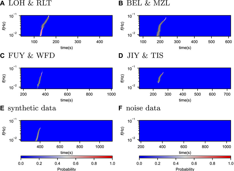
FIGURE 6. Predictions by Surf-Net for the six examples shown in Figure 4. It is in the same presentation way as Figure 4 but with shaded black regions centered around the labeled arrival times with a half-width of 5 times the σ.
We average all the single dispersion curves from the same station pair to obtain the final average dispersion curves. Due to noise and cycle skipping, some picks have errors and must be removed. Thus, we discard picks with differences from the median value larger than 2.5 times the quartile deviation (QD) for a specific station pair. When the value of 2.5 times QD is smaller than 1% of the median, the threshold is set to 1% of the median. We do this elimination twice to discard most of the outliers. The corresponding average curve is considered valid if more than four picks remain with a standard deviation smaller than 3%. Figure 7 shows four examples of this process for the same station pairs as in Figure 4. Although a few bad picks remain, they can be eliminated via the outlier removal process mentioned before.
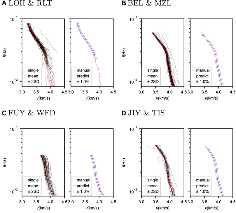
FIGURE 7. Comparisons between the predicted dispersion curves by Surf-Net and manual results for four station pairs. In each subfigure (A–D), the left one shows the predicted single (black lines) and average (solid red lines) dispersion curves with 2 times the standard deviations (dashed red lines), and the right one shows the predicted (red line) and manual (solid blue line) average dispersion curves with a 1% perturbation (dashed blue lines).
To measure the performance of Surf-Net quantitatively, we set the metrics similar to those of PhaseNet (Zhu and Beroza, 2019): the precision P, recall R, F1 score are determined as
where outputs with maximum values higher than 0.5 and velocity differences smaller than the threshold are counted as True Positive (Tp); outputs with maximum values higher than 0.5 and velocity differences larger than the threshold are counted as False Positive (Fp); the other outputs are counted as False Negative (Fn). The picks with differences smaller than 3 times the threshold are used for calculating the mean(μ) and standard deviation(σ). We set different thresholds for different datasets due to their label quality. For the synthetic data, the threshold is 1% as the labels are strictly right. For single picks of observational data, the threshold is 1.5% as they can be affected by noise and measurement error. For average picks of the observational data, the threshold is 1%, as the extraction error can be reduced by averaging. Surf-Net is trained and tested three times to obtain the standard deviations.
We first test Surf-Net on the synthetic data to show its extraction accuracy for various dispersion curves compared to the MFT. Next, we test Surf-Net on the observational data to show its practicability in applications, especially the ability to remove invalid picks. Considering that the manual removal of invalid picks is not always correct, we do not measure how correctly the method handles the invalid picks by using the discarded picks. Instead, we use the performance for the average dispersion curves to examine whether Surf-Net can eliminate the invalid picks or not. If the model can handle the invalid picks correctly, the predicted average dispersion curves should be close to the manual ones. Otherwise, there should be noticeable differences. To make the test more reliable, we also applied our method to unlabeled observational samples from the same station pairs to get the final average dispersion curves. Including the original labeled samples, the numbers of used CC samples for station pairs in the training, validation, and test sets are 47,116, 5887 and 5544, respectively. Part of the unlabeled samples has noticeable noise, which realistically tests our method.
To measure how the distance information and large-kernel convolution layer affect the performance, we test two new models called ‘Surf-Net_noDis’ and ‘Surf-Net_small’. One has the same structure as Surf-Net but is trained with the input distance channel set to zero. For the other model, the large-kernel convolution layer is replaced with a small-kernel convolution layer with a kernel size of 8. To keep the parameter amounts of Surf-Net and Surf-Net_small approximately equal, we expand Surf-Net_small’s channel numbers of every level to 80, 75, 70, 60, 50, 40 and 40.
To illustrate the effect of different training sets, we train and test the model using observational and synthetic data, respectively. The above two models are respectively called ‘Surf-Net_obs’ and ‘Surf-Net_syn’.
As a reference for tests, we also carry out a conventional automatic selection method based on the signal-to-noise ratios and the differences in velocity and its gradient
To further show Surf-Net’s potential in practical applications, we compare the tomography results derived from the predicted and manually-obtained dispersion curves. We also applied our method in Southeast China and compared its tomography results with previously published models (Shen et al., 2016; Han et al., 2021).
The performances of Surf-Net, Surf-Net_noDis, Surf-Net_small, Surf-Net_obs, Surf-Net_syn, and MFT for single picks of synthetic data in the test set are listed in Table 1 and their error distributions and performance at different frequencies are shown in Figure 8. The general result in Table 1 shows that for synthetic data with added noise, Surf-Net and Surf-Net_syn perform better than other methods.
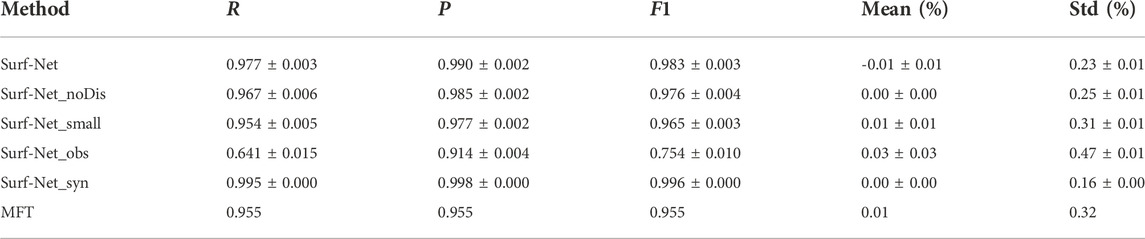
TABLE 1. Performance for single picks in the synthetic test set. The threshold is set to 1%.
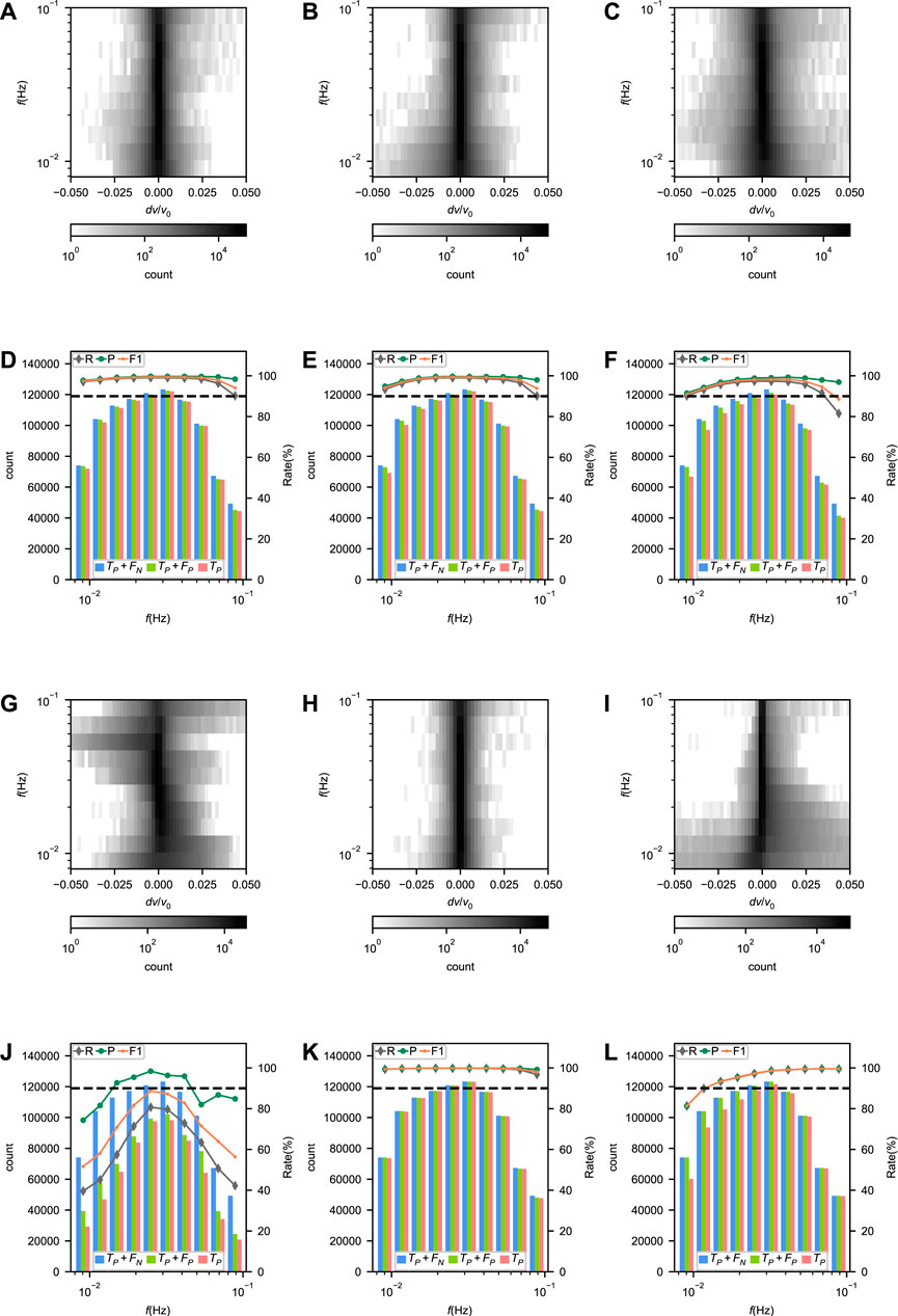
FIGURE 8. (A–C) and (G–I) Error distributions and (D–F) and (J–L) performances of Surf-Net (A, D), Surf-Net_noDis (B, E), Surf-Net_small (C, F), Surf-Net_obs (G, J), surf-Net_syn (H, K) and MFT (I, L) at different frequencies for the single picks in the synthetic test set. In (A–C, G–I), the shades of grey show the number of picks with close measurement errors for the same frequency. In (D–F, J–L), the histograms represent the values of Tp, Tp + Fp and Tp for different frequencies corresponding to the left vertical axes. The lines of three colors respectively represent the recall, precision and F1 corresponding to the right vertical axes. The black dashed line shows the rate of 90%.
As Figure 8D shows, the precision of Surf-Net keeps high at all frequencies. However, affected by the high drop rate of the observational data at high frequencies (Figure 3B), Surf-Net is more likely to drop picks at high frequencies and the recall decreases, although the weights of dropped channels have already been adjusted according to the drop rates.
Compared with the Surf-Net, Surf-Net_noDis (Table 1; Figure 8E) has a slightly worse performance at low frequencies. Surf-Net_small also performs worse than Surf-Net, and its picking errors spread wider (Table 1; Figures 8C, F). These two tests show the advantage of involving distance information and using the large-kernel convolution layer.
Although the recall of Surf-Net_obs on the synthetic data falls obviously, its precision keeps above 90% (Table 1). The performance drop is mainly due to the difference between the observational and synthetic data. However, the precision higher than 90% still shows our method’s generalization ability in some way. The performance distribution along the frequency (Figure 8J) shows that Surf-Net_obs performs better in the middle frequency range than in others, as there are more labelled data in the middle frequency range (Figure 2). Surf-Net_syn has the best performance for the single picks in the synthetic test set. Trained by the synthetic and observational data, Surf-Net achieves a slightly worse performance than Surf-Net_syn (Table 1). As the synthetic data are strictly right while some observational data are of obvious error, this slight performance degradation for synthetic data after adding observational data is normal.
Compared with the MFT (Figures 8I,L), Surf-Net has a significant advantage at low frequencies. To illustrate these performance differences, we give three synthetic examples in Figure 9. Surf-Net and the MFT are applied on cross-correlation waveforms with and without noise. While both Surf-Net and MFT work well on the original CCs, the MFT gives dispersion curves of larger errors at the low frequencies for the noised CCs than Surf-Net. For waves at low frequencies, MFT often uses long time windows which easily involve more noise and thus result in measurement errors. It shows that Surf-Net has learned how to extract dispersion curves in a robust way to reduce noise effects.
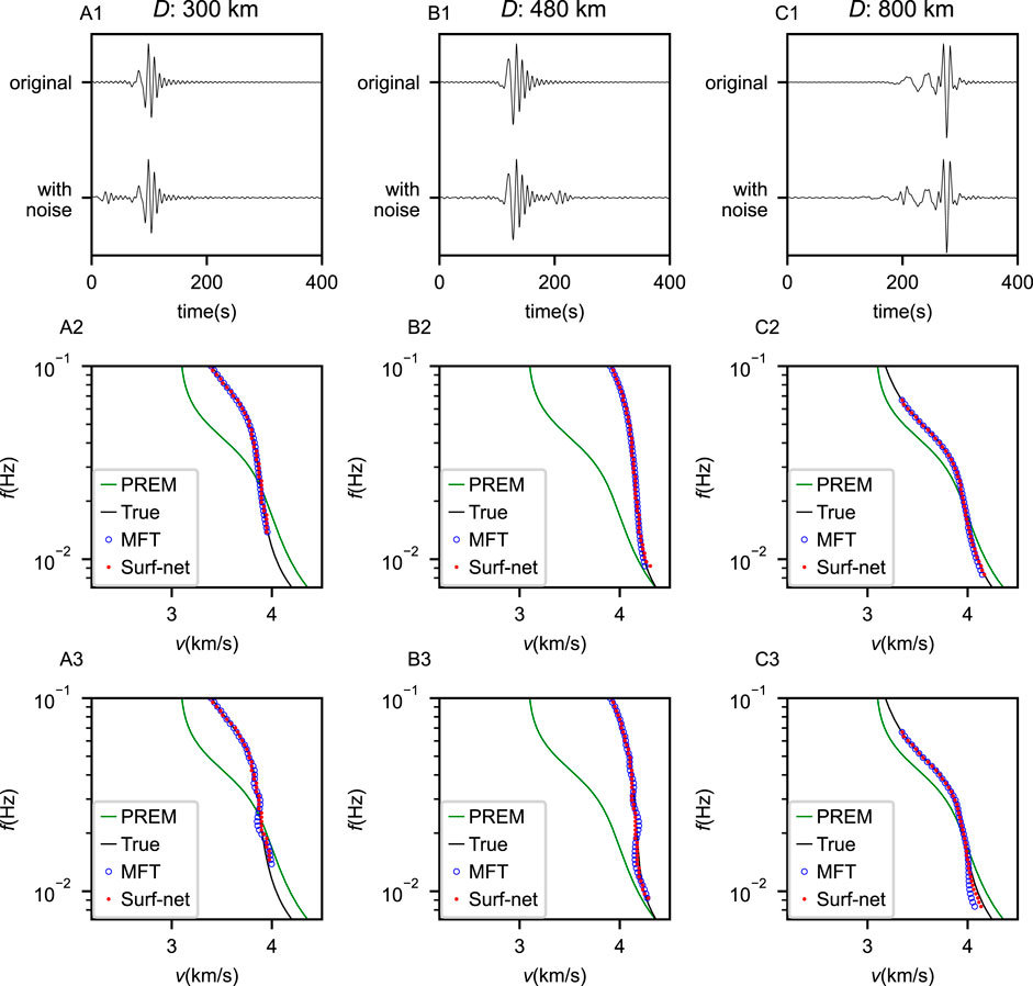
FIGURE 9. Three examples of synthetic data and extractions from them. In each example (A1-3–C1-3), the first trace in the top plot (A1–C1) is an original synthetic cross-correlation waveform corresponding to a chosen dispersion curve shown by black lines in the mid (A2–C2) and bottom plots (A3–C3) while the second trace marked in the top plot (A1–C1) is generated by adding noise before or after the primary wavelet to the original waveform. The picking results from the MFT and Surf-Net on the original and noised waveforms are shown in the mid (A2–C2) and bottom (A3–C3) plots, respectively.
On our workstation, Surf-Net process all the observational cross-correlation waveforms using about 238 s while the conventional method costs about 4,115 s. The performances of Surf-Net, Surf-Net_noDis, Surf-Net_small, Surf-Net_obs, Surf-Net_syn and the conventional method for single and average picks in the observational test set are summarized in Tables 2, 3, respectively. The corresponding error distributions and performance at different frequencies are shown in Figures 10, 11. Picks of several station pairs by the above methods are shown in Figure 7, S2,S3,S4, S5 and S6,respectively.
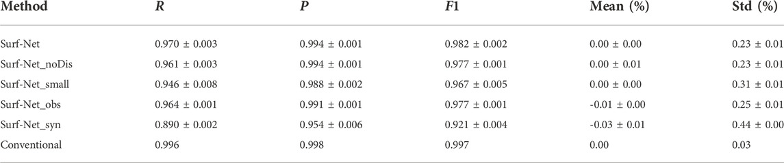
TABLE 2. Performance for single picks in the observational test set. The threshold is set to 1.5%.
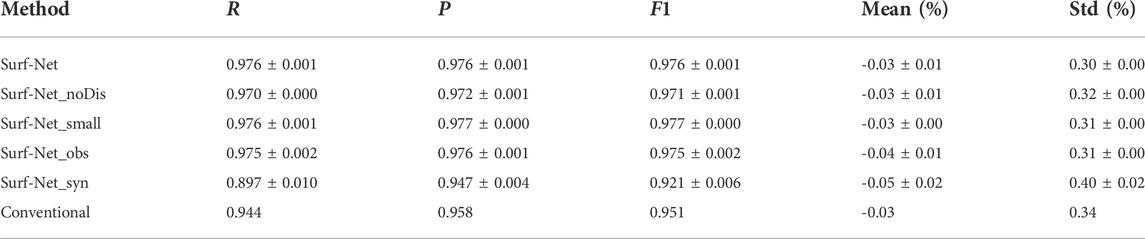
TABLE 3. Performance of average picks in the observational test set. The threshold is set to 1%.
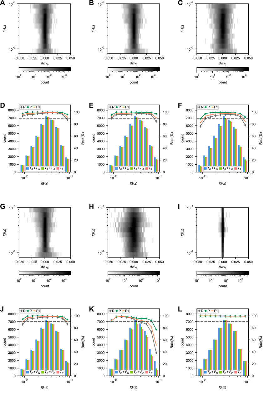
FIGURE 10. (A–C) and (G–I) Error distributions and (D–F) and (J–L) performances of Surf-Net (A,D), Surf-Net_noDis (B,E), Surf-Net_small (C,F), Surf-Net_obs (G,J), surf-Net_syn (H,K) and the conventional method (I and L) at different frequencies for the single picks in the observational test set.
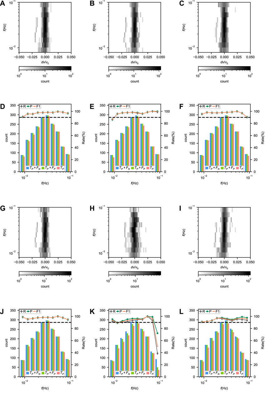
FIGURE 11. (A–C) and (G–I) Error distributions and (D–F) and (J–L) performances of Surf-Net (A, D), Surf-Net_noDis (B,E), Surf-Net_small (C,F), Surf-Net_obs (G,J), surf-Net_syn (H,K) and the conventional method (I,L) at different frequencies for the average picks in the observational test set.
For Surf-Net, the precision of single picks is high, while the recall is a little lower, showing that most single dispersion curves are picked accurately, and part of the labeled picks are discarded. The errors at different frequencies are distributed around zero (Figure 10A). Due to the high drop rates (Figure 3B) and small sample numbers, the recalls at the lowest and highest frequencies are relatively low.
Like the examples in Figure 7, there are few bad picks in those extracted by Surf-Net. Metrics on the average picks (Table 3) show that Surf-Net can provide similar results to the manual ones. The errors at different frequencies are also distributed around zero (Figure 11A). Although part of the labeled single picks is discarded, other samples can cover the frequency range, making the recall drop around low and high frequencies smaller. As shown in Figures 11D, L, Surf-Net performs better than the conventional method at low frequencies, which is consistent with the synthetic test and thus can help get a better resolution for velocity structures at large depths.
For Surf-Net_noDis, its performance for both single and average picks is lower than Surf-Net (Table 2,3), showing it is necessary to input the distance information. As examples in Supplementary Figure S2 show, Surf-Net_noDis has more possibility to give bad picks with apparent errors. However, it can provide the right picks in most cases, and the final average results were not heavily affected when the outlier removal was applied. It is worth noting that the performance of Surf-Net_noDis is almost good enough, which perhaps means the model can estimate the distance by the input CC or determine the actual arrival time according to the wave packet. However, factors like noise may affect this estimation or determination and thus generate bad picks.
Surf-Net_small’s performance drop for single picks is more obvious than Surface-Net_noDis (Table 2; Figure 10). It demonstrates the improvements by using the large-kernel convolution layer. However, as Surf-Net_small takes the distance information into account, it provides fewer false detections than Surface-Net_noDis (Supplementary Figure S2, 3) and shows a better performance for the average picks (Table 3).
Compared with Surface-Net_obs, Surf-Net has a better performance for single picks (Table 2), showing that the synthetic data containing dispersion curves from various underground seismic velocity structures helps Surf-Net to have a better performance for the observational data. Surface-Net_syn’s performance for single observational picks is better than Surface-Net_obs’s performance for single synthetic picks (Table 1,2), which also indicates the synthetic dataset contains various samples than the observational dataset. However, as the observational waveform’s features are not exactly the same as synthetic ones, Surf-Net_syn provides a lot of false picks (Supplementary Figure S5), showing that the observational data are still needed.
As both the conventional and manual methods are selected from the same single dispersion curves pre-extracted by the MFT method, it is natural that the conventional method’s results have a good consistency with the labeled single picks and remain most of the labeled picks (Table 2). However, as shown in Supplementary Figure S6, it remains a lot of bad picks and thus has a worse performance for the average picks than Surf-Net, especially for picks at low frequencies (Table 3; Figure 11L).
Finally, we examine the performance of Surf-Net in providing surface-wave dispersion curves for seismic tomography. Using the direct inversion method proposed by Liu et al. (2019), we invert for the S-velocity structure with azimuthal anisotropy using the surface wave dispersion curves beneath Northeast China obtained separately by Surf-Net and manual approach. We only use the dispersion curves from the labelled station pairs to make the ray path coverage consistent in the two inversions. The resulting models and their difference are shown in Figure 12, while the checkerboard test and other inversion details are given in Supplementary Information S4.
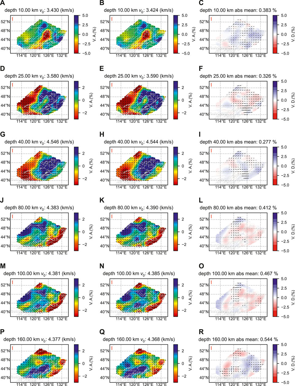
FIGURE 12. Azimuthally anisotropic S-wave velocities for Northeast China obtained from Rayleigh-wave tomography using dispersion curves derived by Surf-Net (left column) and manual (middle column) methods. The right column shows the difference between the two models. Shown here are horizontal slices of the models at depths of 10 km (A–C), 25 km (D–F), 40 km (G–I), 80 km (J–L), 100 km (M–O), and 160 km (P–R). In each subplot, the color represents the relative perturbation of the isotropic S-wave velocity from an average value given at the top, and the short line segments show anisotropy, with length and direction indicating strength and symmetry axes, respectively. The vertical red line in the top left corner of the map shows an anisotropy amplitude of 3%. The light grey lines show the faults.
The two tomography models are almost similar, with the mean absolute difference no larger than 0.544% in the 10–160 km depth range. They have similar velocity patterns: at the depths of 10 km and 25 km, there is an apparent low-velocity anomaly in the middle of the region; at a greater depth of 40 km, we can see that the velocities in the eastern part are higher than in the western part, indicating that the eastern part has a thinner crust; at the depths of 80 km, 100 km, and 160 km, there are apparent low-velocity anomalies in the north and southeast. Moreover, in most cases, the direction and amplitude patterns of the azimuthal anisotropy are similar, with slight differences. However, there are still some minor differences, and most of them are located in the low-resolution part according to the checkerboard test (Supplementary Information S4). This test demonstrates that Surf-Net can provide dispersion curves with reliable structure information.
We show the tomography results from dispersion curves respectively extracted by Surf-Net_obs and Surf-Net_syn in Supplementary Figures S9, 10. The tomography results of Surf-Net_obs are similar to those of Surface-Net. Tomography results of Surf-Net_syn have a slightly larger difference from the manual ones compared to Surf-Net and Surf-Net_obs. Considering Surface-Net_syn’s training uses none of the observational data, its results are good enough.
The tomography results of Surf-Net in Southeast China are similar to two previously published models (Supplementary Figure S12). The velocity model in the shallow depth is consistent with the surface structure. The tomography results also show the difference between the eastern and western areas and the correlation between the deep and shallow structures. Considering the three models are not from the same data and inversion methods, the differences among them are acceptable. As the geological environments of Southeast and Northeast China are different, this application demonstrates Surf-Net’s good generalization ability and potential to be used in other areas.
Taking the velocity measurement task as an arrival time picking problem and making good use of the waveform information, we have developed Surf-Net, a deep-learning-based neural network. It is designed to extract and select dispersion curves directly from the waveform cross-correlations and distance information. Trained by the synthetic data and manually selected observational data, the network can extract the dispersion curves accurately and remove bad picks successfully.
According to the test on the synthetic data, Surf-Net has learned a robust way to extract dispersion curves with higher accuracy than the MFT method, especially for low frequencies. Evaluated with observational data for both single and average dispersion curves, Surf-Net shows the ability to provide reliable single picks with a limited number of bad picks and average dispersion curves with higher accuracy than the conventional method. The performance advantage at low frequencies is significant too.
The comparison among different types of Surf-Nets shows the improvements from the distance information and large-kernel convolution layer. The performance differences among Surf-Nets trained with different datasets show that the synthetic data is useful in training a better model.
The comparison between the tomography results demonstrates that Surf-Net can provide dispersion curves with reliable underground structure information. The application in Southeast China shows Surf-Net’s potential to be used in other areas. Furthermore, also provides a general framework for other surface-wave analyses, such as the extraction of Love-wave dispersion curves and measurement of dispersion curves of overtones.
The observational seismic data used is from the Earthquake Science Data Center, Institute of Geophysics, China Earthquake Administration and is only available to researchers and graduate students in China after signing the “Seismic Waveform Data Sharing Agreement of the Earth Science Data Center”. The Email address for contacting the center isNDQ2MTkxQHFxLmNvbQ==. The extracted dispersion curves and generated synthetic waveform data are available online(https://doi.org/10.5281/zenodo.7335287). Further inquiries can be directed to the corresponding author.
JN proposed the initial idea and guided the whole research. YJ proposed the initial design of the deep learning model and improved it. JW gave the basic knowledge of surface wave extraction and participated in the model improvement and the result analysis. YT, MW, TZ, and TB selected the dispersion curves and provided knowledge of the conventional methods. TZ, JL, YS, and HW participated in the article organization and writing.
This work was supported by National Science Foundation of China under grant No. 41874071 and High-performance Computing Platform of Peking University.
The authors thank the Earthquake Science Data Center, Institute of Geophysics, China Earthquake Administration for providing the observational seismic data. The authors acknowledge the course ‘English Presentation for Geophysical Research’ of Peking University (Course #01201110) for help in improving the manuscript.
Author TZ was employed by the Aramco Asia.
The remaining authors declare that the research was conducted in the absence of any commercial or financial relationships that could be construed as a potential conflict of interest.
All claims expressed in this article are solely those of the authors and do not necessarily represent those of their affiliated organizations, or those of the publisher, the editors and the reviewers. Any product that may be evaluated in this article, or claim that may be made by its manufacturer, is not guaranteed or endorsed by the publisher.
The Supplementary Material for this article can be found online at: https://www.frontiersin.org/articles/10.3389/feart.2022.1030326/full#supplementary-material
Bensen, G., Ritzwoller, M., Barmin, M., Levshin, A., Lin, F., Moschetti, M., et al. (2007). Processing seismic ambient noise data to obtain reliable broad-band surface wave dispersion measurements. Geophys. J. Int. 169, 1239–1260. doi:10.1111/j.1365-246X.2007.03374.x
Bridle, J. (1990). “Training stochastic model recognition algorithms as networks can lead to maximum mutual information estimation of parameters,” in Advances in Neural Information Processing Systems 2, San Francisco, CA: Morgan Kaufmann Publishers Inc., 211–217.
Cheng, B., and Titterington, D. M. (1994). Neural networks: A review from a statistical perspective. Stat. Sci. 9, 2–30. doi:10.1214/ss/1177010638
Chollet, F. (2017). “Xception: Deep Learning with Depthwise Separable Convolutions,” in Proceedings of the 2017 IEEE Conference on Computer Vision and Pattern Recognition (CVPR), Honolulu, HI: IEEE, 1800–1807. doi:10.1109/CVPR.2017.195
Dai, T., Xia, J., Ning, L., Xi, C., Liu, Y., and Xing, H. (2021). Deep learning for extracting dispersion curves. Surv. Geophys. 42, 69–95. doi:10.1007/s10712-020-09615-3
Ding, X., Zhang, X., Han, J., and Ding, G. (2022). “Scaling up your kernels to 31x31: Revisiting large kernel design in cnns,” in Proceedings of the 2022 IEEE/CVF Conference on Computer Vision and Pattern Recognition, New Orleans, LA: IEEE, 11963–11975.
Dong, S., Li, Z., Chen, X., and Fu, L. (2021). DisperNet: An effective method of extracting and classifying the dispersion curves in the frequency–Bessel dispersion spectrum. Bull. Seismol. Soc. Am. 111, 3420–3431. doi:10.1785/0120210033
Dziewonski, A., and Hales, A. (1972). “Numerical analysis of dispersed seismic waves,” in Seismology: Surface waves and Earth oscillations, of Methods in computational physics: Advances in Research and applications. Editor B. A. Bolt (Elsevier), 11, 39–85. doi:10.1016/B978-0-12-460811-5.50007-6
Gibbs, M. N., and MacKay, D. J. (2000). Variational Gaussian process classifiers. IEEE Trans. Neural Netw. 11, 1458–1464. doi:10.1109/72.883477
Glorot, X., Bordes, A., and Bengio, Y. (2011). “Deep sparse rectifier neural networks,” in Proceedings of the Fourteenth International Conference on Artificial Intelligence and Statistics, Fort Lauderdale, FL: PMLR, 315–323.
Han, S., Zhang, H., Xin, H., Shen, W., and Yao, H. (2021). USTClitho2.0: Updated unified seismic tomography models for continental China lithosphere from joint inversion of Body-Wave arrival times and Surface-Wave dispersion data. Seismol. Res. Lett. 93, 201–215. doi:10.1785/0220210122
Ioffe, S. (2017). “Batch renormalization: Towards reducing minibatch dependence in batch-normalized models,” in Advances in Neural Information Processing Systems 30, Long Beach, CA: Curran Associates, Inc., 1945–1953.
Jia, Y., and Ma, J. (2017). What can machine learning do for seismic data processing? An interpolation application. Geophysics 82, 163–177. doi:10.1190/geo2016-0300.1
Knopoff, L. (1972). Observation and inversion of surface-wave dispersion. Tectonophysics 13, 497–519. doi:10.1016/0040-1951(72)90035-2
Kovach, R. L. (1978). Seismic surface waves and crustal and upper mantle structure. Rev. Geophys. 16, 1–13. doi:10.1029/rg016i001p00001
Lei, W., Ruan, Y., Bozdağ, E., Peter, D., Lefebvre, M., Komatitsch, D., et al. (2020). Global adjoint tomography—Model GLAD-M25. Geophys. J. Int. 223, 1–21. doi:10.1093/gji/ggaa253
Li, Z., and Chen, X. (2020). An effective method to extract overtones of surface wave from array seismic records of earthquake events. J. Geophys. Res. Solid Earth 125, e18511. doi:10.1029/2019jb018511
Lin, F., Ritzwoller, M. H., and Snieder, R. (2009). Eikonal tomography: Surface wave tomography by phase front tracking across a regional broad-band seismic array. Geophys. J. Int. 177, 1091–1110. doi:10.1111/j.1365-246X.2009.04105.x
Little, W. A. (1974). The existence of persistent states in the brain. Math. Biosci. 19, 101–120. doi:10.1016/0025-5564(74)90031-5
Liu, C., Yao, H., Yang, H., Shen, W., Fang, H., Hu, S., et al. (2019). Direct inversion for three-dimensional shear wave speed azimuthal anisotropy based on surface wave ray tracing: Methodology and application to Yunnan, southwest China. J. Geophys. Res. Solid Earth 124, 11394–11413. doi:10.1029/2018JB016920
Liu, F., Jiang, Y., Ning, J., Zhang, J., and Zhao, Y. (2020). An array-assisted deep learning approach to seismic phase-picking. Chin. Sci. Bull. 65, 1016–1026. doi:10.1360/TB-2019-0608
Meier, T., Dietrich, K., Stöckhert, B., and Harjes, H. (2004). One-dimensional models of shear wave velocity for the eastern Mediterranean obtained from the inversion of Rayleigh wave phase velocities and tectonic implications. Geophys. J. Int. 156, 45–58. doi:10.1111/j.1365-246x.2004.02121.x
Park, C. B., Miller, R. D., Xia, J., and Ivanov, J. (2007). Multichannel analysis of surface waves (MASW)—Active and passive methods. Lead. Edge 26, 60–64. doi:10.1190/1.2431832
Park, C. B., Miller, R. D., and Xia, J. (1999). Multichannel analysis of surface waves. Geophysics 64, 800–808. doi:10.1190/1.1444590
Ronneberger, O., Fischer, P., and Brox, T. (2015). “U-net: Convolutional networks for biomedical image segmentation,” in International conference on medical image computing and computer-assisted intervention (Springer), 234–241.
Sato, Y. (1955). Analysis of dispersed surface waves by means of Fourier transform I. Bull. Earthq. Res. Inst. 33, 33–48.
Shapiro, N. M., and Ritzwoller, M. H. (2002). Monte-Carlo inversion for a global shear-velocity model of the crust and upper mantle. Geophys. J. Int. 151, 88–105. doi:10.1046/j.1365-246x.2002.01742.x
Shen, W., Ritzwoller, M. H., Kang, D., Kim, Y., Lin, F., Ning, J., et al. (2016). A seismic reference model for the crust and uppermost mantle beneath China from surface wave dispersion. Geophys. J. Int. 206, 954–979. doi:10.1093/gji/ggw175
Tian, Y., Legendre, C. P., Zhou, T., Han, J., Wu, M., Zhao, L., et al. (2017). High resolution anisotropic phase velocity tomography of Northeast China and its implication. Chin. J. Geophys. 60, 1659–1675.
Trampert, J., and Woodhouse, J. H. (1996). High resolution global phase velocity distributions. Geophys. Res. Lett. 23, 21–24. doi:10.1029/95gl03391
Ulyanov, D., Vedaldi, A., and Lempitsky, V. (2016). Instance normalization: The missing ingredient for fast stylization. doi:10.48550/ARXIV.1607.08022
Xia, J., Miller, R. D., and Park, C. B. (1999). Estimation of near-surface shear-wave velocity by inversion of Rayleigh waves. Geophysics 64, 691–700. doi:10.1190/1.1444578
Yang, S., Zhang, H., Gu, N., Gao, J., Xu, J., Jin, J., et al. (2022). Automatically extracting surface-wave group and phase velocity dispersion curves from dispersion spectrograms using a convolutional neural network. Seismol. Res. Lett. 93, 1549–1563. doi:10.1785/0220210280
Yao, H., van der Hilst, R. D., and de Hoop, M. V. (2006). Surface-wave array tomography in SE Tibet from ambient seismic noise and two-station analysis - I. Phase velocity maps. Geophys. J. Int. 166, 732–744. doi:10.1111/j.1365-246x.2006.03028.x
Yong, H., Huang, J., Meng, D., Hua, X., and Zhang, L. (2020). “Momentum batch normalization for deep learning with small batch size,” in Computer Vision – ECCV 2020: 16th European Conference, Glasgow, United Kingdom, August 23–28, 2020 Proceedings, Part XII, Glasgow: Springer-Verlag, 224–240. doi:10.1007/978-3-030-58610-2_14
Zhang, X., Jia, Z., Ross, Z. E., and Clayton, R. W. (2020). Extracting dispersion curves from ambient noise correlations using deep learning. IEEE Trans. Geosci. Remote Sens. 58, 8932–8939. doi:10.1109/TGRS.2020.2992043
Zhao, M., Chen, S., Fang, L., and Yuen, D. A. (2019). Earthquake phase arrival auto-picking based on U-shaped convolutional neural network. Chin. J. Geophys. 62, 3034–3042.
Zhou, Y., Yue, H., Kong, Q., and Zhou, S. (2019). Hybrid event detection and phase-picking algorithm using convolutional and recurrent neural networks. Seismol. Res. Lett. 90, 1079–1087. doi:10.1785/0220180319
Zhu, W., and Beroza, G. C. (2019). PhaseNet: A deep-neural-network-based seismic arrival-time picking method. Geophys. J. Int. 216, 261–273.
Keywords: surface wave dispersion curve, deep learning, automatic extraction, data processing, Northeast China
Citation: Jiang Y, Wen J, Tian Y, Wu M, Ning J, Shi Y, Wu H, Zhou T, Li J and Bao T (2023) Surf-Net: A deep-learning-based method for extracting surface-wave dispersion curves. Front. Earth Sci. 10:1030326. doi: 10.3389/feart.2022.1030326
Received: 28 August 2022; Accepted: 10 November 2022;
Published: 11 January 2023.
Edited by:
Dun Wang, China University of Geosciences Wuhan, ChinaReviewed by:
Yibo Wang, Institute of Geology and Geophysics (CAS), ChinaCopyright © 2023 Jiang, Wen, Tian, Wu, Ning, Shi, Wu, Zhou, Li and Bao. This is an open-access article distributed under the terms of the Creative Commons Attribution License (CC BY). The use, distribution or reproduction in other forums is permitted, provided the original author(s) and the copyright owner(s) are credited and that the original publication in this journal is cited, in accordance with accepted academic practice. No use, distribution or reproduction is permitted which does not comply with these terms.
*Correspondence: Jieyuan Ning, bmp5QHBrdS5lZHUuY24=
Disclaimer: All claims expressed in this article are solely those of the authors and do not necessarily represent those of their affiliated organizations, or those of the publisher, the editors and the reviewers. Any product that may be evaluated in this article or claim that may be made by its manufacturer is not guaranteed or endorsed by the publisher.
Research integrity at Frontiers
Learn more about the work of our research integrity team to safeguard the quality of each article we publish.