Machine learning opportunities to conduct high-fidelity earthquake simulations in multi-scale heterogeneous geology

The 2019 Le Teil earthquake is an illustrative example of a moderate (M_W 4.9) yet damaging event, occurring at shallow depth (≈1 km) in a region with little to no geophysical data available. Therefore, using a high-fidelity wave propagation code, we performed numerical simulations of the Le Teil earthquake in a highly uncertain framework, investigating several seismic sources and geological set-ups. With respect to the former aspect, a point-source model and an extended kinematic fault model were compared. The latter aspect was investigated by comparing a 1D-layered to a 3D geological model. Those models were enhanced with random fluctuations, in order to obtain three alternative non-stationary random geological fields. The synthetic waveforms obtained from regional geophysical models were globally coherent with the recorded ones. The extended fault source model seemed more realistic than the point-source model. In addition, some geological random fields improved the synthetics’ agreement with the recordings. However, the three random field samplings led to a high variability in induced ground motion responses. Given the computational burden of high-fidelity simulations, we used two dimensionality reduction methods, namely the Principal Component Analysis (PCA) and a deep neural network (3D UNet), to investigate this variability. The methods were applied to a database of 40,000 3D geological random fields. Both the PCA and the 3D UNet condensed the variability of the 3D geological fields into a few components. These were sufficient to reconstruct the original fields with great accuracy. More importantly, the seismic response arising from the propagation throughout the reconstructed fields was in excellent agreement with the response of the original geological fields in more than 75% of the dataset. By building a structured ensemble of complex geological fields from their reduced representation, it may become possible to find a relationship between the reduced representation and the generated ground motion. Thus, our study proves the interest of dimensionality reduction to perform uncertainty analyses in complex geological media.

1 Introduction

The current availability of large computational resources makes three-dimensional (3D) high-fidelity earthquake simulations affordable for intensive computation across wide regions. A large amount of scenarios can be investigated for a specific site, with sufficient accuracy, e.g. up to 10 Hz, and at a reasonable computational cost (Maufroy et al., 2016; Shen et al., 2022; Touhami et al., 2022). However, numerical models must be fed with accurate information on the parameters at stake to obtain results as realistic as possible. The need for a detailed geophysical (P- and S-wave velocities, density, anelastic attenuation) and seismological (fault geometry, focal mechanism, slip patch, rupture path) description of the region under study has for long been acknowledged, but often not met (Hollender et al., 2018). Such large parameter uncertainties prevent the exploitation of the full potential of modern computer software, capable of reproducing complex seismic wave propagation with high accuracy when correctly constrained.

The need for accurate parameters poses considerable challenges, especially in regions with a low-to-moderate seismicity such as southeastern France. The Rhône valley was hit by a M_W4.9 earthquake on 11 November 2019 known as the Le Teil earthquake. While the seismic source can be constrained by InSAR data (De Novellis et al., 2020; Vallage et al., 2021), determining local geological models is more challenging. In this region with a low instrumental seismicity (Larroque et al., 2021), poor geological measurements are available at present. Although geophysical campaigns were conducted after the earthquake, data remain too sparse to design a geological model at the scale of interest (Marconato et al., 2022). Therefore, the most specific geological model is the 3D regional velocity model (P- and S-waves) recently elaborated within the framework of the SIGMA2 international project (Arroucau 2020). Thus, in the absence of a validated local model, it is legitimate to explore the abilities of regional-scale models in regional numerical simulations.

However, due to its insufficient resolution, this 3D geological model shows only gentle horizontal variations representing the main geological patterns of the region (i.e. a 70 km × 100 km domain across the Rhône Valley characterized by a crystalline basement with higher velocities in the Massif Central in the Northwest and sediments in the plain (Ritz et al., 2020)). The 3D model especially lacks the description of the sedimentary basin extending along the Rhône valley (Bravard and Gaydou 2015). This prevents the possibility to constrain numerical simulations in a broad-band spectrum (0–10 Hz at least). One possible remedy consists in modelling the sedimentary basin from a Digital Elevation Model. Then, velocity fields can be inferred from 1D velocity profiles acquired by seismic inversion inside and outside the basin, as done by Smerzini et al., 2022; Haber, 2021. This method has already been adopted in other low-to-moderate seismicity regions such as the Grenoble region (Chaljub 2006; Stupazzini et al., 2009).

Another modelling challenge is introduced by small-scale heterogeneity, which plays a crucial role in seismic wave propagation, especially at high-frequency (Vyas et al., 2018; Scalise et al., 2021). Heterogeneity is rarely included in numerical simulations due to the increased computational demand. It can be represented by random fields that add small scale fluctuations to the geophysical models (Gatti et al., 2017; Svay et al., 2017). For uncertainty quantification purposes though, a large number of simulations is necessary. Yet the cost of high-fidelity simulations on large and complex domains - increasing with spatial resolution - prevents computationally demanding approaches such as Monte Carlo methods.

Conducting uncertainty analyses while maintaining affordable computation costs therefore raises the question of how to reduce the dimensionality of such refined geophysical descriptions. To this end, autoencoders are among the most popular deep learning methods to reduce the dimensionality of inputs (Hinton and Salakhutdinov 2006). They can be viewed as a nonlinear extension of the well known Principal Component Analysis (PCA). Autoencoders have been largely used in various fields to encode complex datasets into reduced order manifolds (e.g., Ladjal et al., 2019; Kadeethum et al., 2022), but their application on 3D data remains spurious (Gangopadhyay et al., 2021; Tekawade et al., 2021; Yu et al., 2021). In seismology, Cheng and Jiang 2020 used a Conditional Variational Auto-Encoder to obtain a geophysical model of the Earth crust in Tibet. The encoder mapped Rayleigh surface waves into parameters representing the thickness, P- and S-waves velocities, and density in several layers while the decoder ensured that those parameters were meaningful for reconstructing the original surface waves. Additionally, Zeng et al., 2021 performed seismic waveform inversion using an autoencoder structure augmented with inversion layers.

On the one hand, this study extends the classical physics-based numerical validation of a past earthquake by adding random fluctuations to the mean geological configuration (Figure 1A). On the other hand, it attempts a dimensionality reduction of the geological fields, towards the definition of eigengeologies that mostly influence the propagated wave motion (Figure 1B). Firstly, we compare two regional low-resolution geological models to simulate the Le Teil earthquake for a point-source and an extended fault source. Secondly, random fluctuations are added to the best-fitting geological model. This assesses the impact of different random field samplings on the propagated ground motion at the surface. Then, given the large variability of the simulated ground motion, we propose a method to represent 3D complex geological media with the smallest dimensionality possible. To this end, we construct a learning database of 40,000 3D heterogeneous geological models and we compare the performances of the PCA and of the 3D autoencoder proposed by Çiçek et al., 2016 (3D UNet) in reducing the dimensionality. With this approach, we show that it is possible to encode the geological database into a few number of meaningful features. Once decoded, those features generate very good reconstructions of the initial database that retain all the necessary information without degrading the propagated seismic response.

FIGURE 1

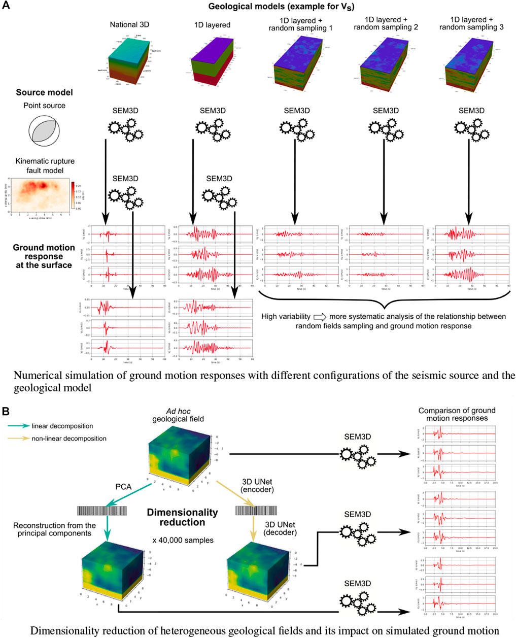
FIGURE 1. Workflow of this study. (A) corresponds to Section 2 and Section 3 while (B) refers to the work done in Section 4 and Section 5.

In the following study, Section 2 describes the numerical model used to simulate the Le Teil earthquake while results are presented in Section 3. Then, Section 4 details the geological database and the dimensionality reduction methods. Outputs of these methods are analyzed in Section 5. The discussion in Section 6 concludes the manuscript.

1) Numerical simulation of ground motion responses with different configurations of the seismic source and the geological model.

2) Dimensionality reduction of heterogeneous geological fields and its impact on simulated ground motion.

2 Data and methods for the simulation of seismic wave propagation

2.1 The Le Teil earthquake case study

The Le Teil earthquake occurred on 11 November 2019 on the La Rouvière fault, a fault which was not considered as active despite being part of the larger Cevennes fault system which was potentially active (Ritz et al., 2020). To date, the Le Teil earthquake is the most damaging earthquake of the last decades in Metropolitan France. Remarkably, this shallow earthquake (1.3 km depth ±0.5 km) induced a surface rupture. Figure 2 shows the map of the region of interest, including the available recording stations and the trace of the la Rouvière fault.

FIGURE 2

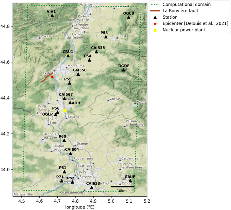
FIGURE 2. Map of the region affected by the 2019 Le Teil earthquake, in South-Eastern France. The computational domain considered in this paper is indicated with the dotted box. Velocimeters and accelerometers are shown with black triangles (details in Supplementary Table S1).

The Le Teil earthquake was recorded over 22 stations within 70 km from the fault (Supplementary Table S1). Some velocimeters (e.g. PAUL and BOLL in Figure 2) saturated while recording and they could not be considered for further analyses. This study focuses on stations located out of the sedimentary basin (OGDF, OGCB, CRU1) since its absence from our models is likely to impact synthetic ground motions inside the basin.

The hypocenter was obtained from the results of the waveform inversion (44.5188° N, 4.6694° E, depth -1.3 km, see Delouis et al., 2021). In this study, two types of seismic sources were compared, with a target seismic moment M₀ = 2.47 ⋅ 10¹⁶ N.m. Namely, a double-couple point source was assumed with strike = 48°, dip = 45°, and rake = 88° (Delouis et al., 2021). Its source time function is given by

$t\mapsto 1-\left(1+\frac{t}{\tau }\right)e^{-\frac{t}{\tau }},(1)$

with $\tau =10^{0.5(M_W-6.69)}$ = 0.127 s (Dreger and Douglas, 2007; Gatti, 2017). In addition, a kinematic fault model was designed from the inversion of InSAR satellite observations performed by Vallage et al., 2021 (see Figure 3). The fault model was computed following the Ruiz’s Integral Kinematic (RIK) numerical scheme (Ruiz et al., 2011) implemented by Gallovič 2016. The fault was represented as a 7 km-long and 4 km-deep plane with a 60° dip and reaching the surface at its highest point. It was further discretized in triangular patches. A bidirectional rupture front starts from the nucleation point located at the hypocenter. Each patch activates when it is reached by the rupture front, under the constraint that its final slip corresponds to the one obtained from the InSAR inversion.

FIGURE 3

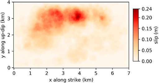
FIGURE 3. Final slip given by the kinematic fault model.

2.2 Geological model

In the absence of a local model, two geological models for metropolitan France were adopted in this study and compared. The first one was a 1D model used by the Geophysical and Detection Laboratory (LDG) of the French Alternative Energies and Atomic Energy Commission (CEA) to locate seismic events (Table 1; Figure 4 and Duverger et al., 2021). It was obtained using the Pg, Sg, Pn, and Sn phases of a series of 50+ well identified earthquakes (Veinante-Delhaye and Santoire, 1980). It presents a thin sedimentary subsurface layer with low velocity (V_S = 1730 m/s), overlying a 25 km thick crustal layer (V_S = 3560 m/s). The average ratio between P- and S- wave velocities is 1.69. The bedrock is described by S-wave velocities of 4650 m/s.

TABLE 1

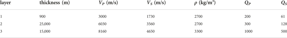
TABLE 1. 1D geological model used by the CEA-LDG to locate seismic events. Described in more details in (Duverger et al., 2021).

FIGURE 4

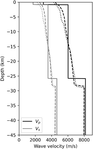
FIGURE 4. V_P (black) and V_S (grey) velocity profiles for the 1D geological model (continuous line), 3D geological model in station VIVF (dashed line), and station SAUF (dotted line).

Alternatively, Arroucau, 2020 proposed in the framework of the SIGMA2 project a 3D velocity model for S- and P-waves in metropolitan France. This model includes topography/bathymetry and was built as an improved and homogeneized version of partial previous models (mainly EPcrust, (Molinari and Morelli 2011), combined with ambient noise and teleseismic surface wave tomography models, a CSS-derived model, and a local earthquake tomography study, see references in (Arroucau 2020)). This model has a 10 km × 10 km × 0.5 km resolution and shows horizontal variability even at the regional scale of interest. Figure 5A for example shows higher surface velocities in the North-Western mountainous part of the region compared to the plains in the South-East. The thickness of the Earth crust is between 26 km and 31 km in the region of interest, consistently with geophysical knowledge (Larroque et al., 2021). This model also leads to a mean V_P/V_S ratio of 1.72 (between 1.68 and 1.8), which is slightly lower than the 1.9 ratio recommended by Delouis et al., 2021 to recover S-waveforms of the Le Teil earthquake.

FIGURE 5

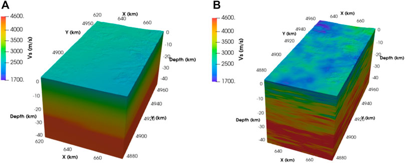
FIGURE 5. 3D geological model for S-wave from (Arroucau 2020). (A) Original model; (B) Addition of random heterogeneities (correlation lengths of 10 km horizontally and 1 km vertically, coefficient of variation of 10%).

2.3 Geological random fields

Acknowledging that regional-scale models cannot be expected to reproduce local specifics, small scale variability was added to the models as random heterogeneities. For this purpose, random fields were generated from a von Karman correlation model (Chernov 1960) with a Hurst exponent of 0.1. The choice of the random fields’ parameters is rather tricky yet of crucial importance (Colvez 2021). Following previous studies (Khazaie et al., 2016; Scalise et al., 2021), we adopted correlation lengths of 10 km in the horizontal direction and 1 km in the vertical direction, associated with a 10% coefficient of variation(see Figure 5B). This parametrization is coherent with the results obtained for the Le Teil earthquake via a Monte-Carlo approach of particles diffusion in a heterogeneous Earth crust (Heller 2021).

The 3D random field computation is made highly efficient by the use of the spectral representation (Shinozuka and Deodatis 1991; de Carvalho Paludo et al., 2019). With this formulation, a centered Gaussian random field u determined by its autocovariance function $\mathcal{R}$ can be decomposed as a sum of independent identically distributed random variables ${({\varphi }_n)}_{-N\le n\le N}$, with uniform distribution over [0, 2π]

$u\left(x\right)=\sum _{n=-N}^N\sqrt{2\widehat{\mathcal{R}}\left(n\mathrm{\Delta }k\right)}\cos \left(n\mathrm{\Delta }k\cdot x+{\varphi }_n\right)$

where $\widehat{\mathcal{R}}$ is the Fourier transform of the autocovariance function $\mathcal{R}$ and Δk the unit volume in ${\mathbb{R}}^3$. Random fields were thus generated in a few seconds for the whole domain with a 2 km × 2 km × 0.2 km resolution. They were later interpolated on the Gauss-Lobato-Legendre (GLL) points as part of the computation process.

2.4 Simulation framework

Numerical simulations were performed using SEM3D (Touhami et al., 2022), a High-Performance Computing wave propagation code based on the Spectral Element Method (SEM, Faccioli et al., 1997; Komatitsch and Tromp 1999). SEM3D shows excellent weak scalability properties between 0 and 10,000 MPI processes and it has been widely employed to simulate past earthquakes and to assess the seismic response of nuclear sites and urban areas (Gatti, 2018; Touhami et al., 2021; Korres et al., 2022). Moreover, SEM3D employs the Convolution-Perfectly-Matched Layers (C-PML) as absorbing boundary conditions (Martin and Komatitsch 2006).

The 80 km × 92 km × 79 km computational domain was discretized on a hexahedral mesh with 18.3 million elements. With a minimum S-wave velocity of 2180 m/s and 5 GLL points per element, this mesh allowed wave propagation up to 5 Hz. Simulations were run on 2048 cores AMD Milan @2.45 GHz (AVX2) operated by the Très Grand Centre de Calcul (TGCC, France). Thanks to this computational power, simulations were obtained in 61,440 h CPUs for 60 s of simulated signal.

3 Numerical results of the Le Teil earthquake simulation

This section presents the simulation results of the Le Teil earthquake obtained with regional geological models of increasing complexity (Section 3.1) and several samplings of random fields (Section 3.2).

3.1 Comparison with records

Numerical results were compared with seismograms records in several stations to evaluate the parameters choices. Firstly, the point-source was used in conjunction with the 1D geological model. Figure 6 then shows that despite the simplicity of the models, the level of agreement is surprisingly good. Indeed, the frequency response spectra show a correct corner frequency around 0.8 Hz, as well as similar slopes and amplitudes. In addition, the wave arrival times are well reproduced by the simulation, thereby proving that the mean velocity on the source-to-site path is correctly modelled. The very first oscillations are also coherent with the records, especially in station OGDF (Supplementary Figure S1).

FIGURE 6

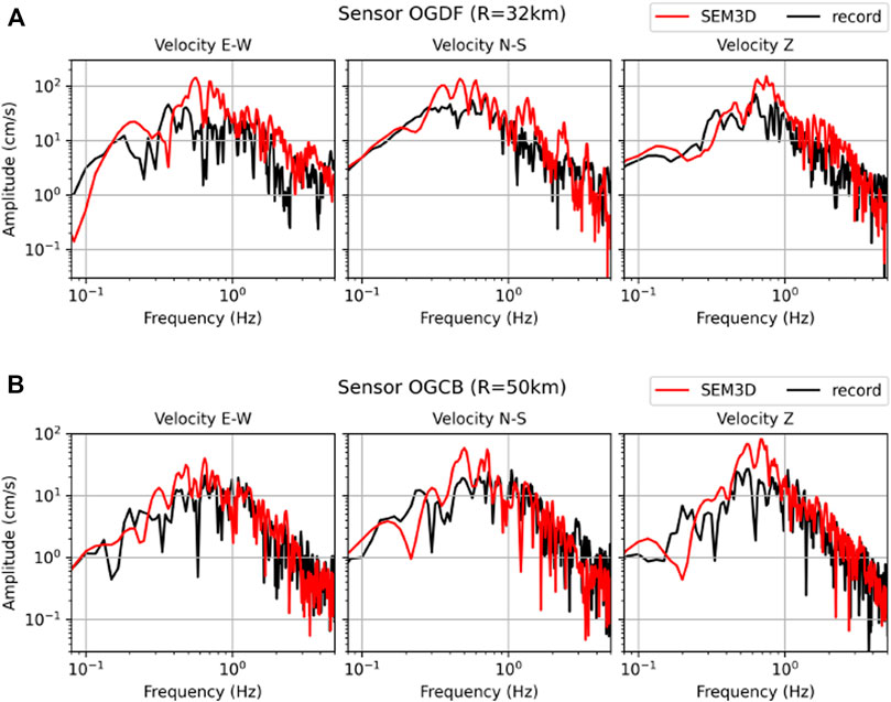
FIGURE 6. Frequency response spectra of the numerical simulation (in red) obtained with the 1D geological model and a point source. Comparison with seismograms records (in black). Velocities are given in the East-West (E-W), North-South (N-S), and vertical (Z) directions for stations OGDF (A) and OGCB (B).

However, one can notice in Supplementary Figures S1A,B that the numerical simulation produces late oscillations with higher amplitudes than the recorded ones. They can be seen from around 27 s in station OGDF and from 36 s in station OGCB. These oscillations may come from the thin upper layer with a high velocity contrast defined in the 1D geological model that creates a wave guide. In fact, when the 3D geological model is used instead of the 1D geological model, those late oscillations are no more present, as can be seen in Supplementary Figures S2A,B.

Yet, the use of the 3D geological model leads to other issues. Supplementary Figures S2A,B indeed show high velocity peaks at the beginning of the signal. The peaks’s amplitude is higher than the maximal velocities recorded during the earthquake. As an example, the horizontal Peak Ground Velocity (PGV) was 5 times higher than records in station OGDF and 7 times higher in station OGCB. The velocity peaks indicate that the energy content of the signal is concentrated with the first wave arrivals. This results from the smoothness of the 3D geological model: the absence of inter-layer discontinuity prevents the multiple wave refractions and reflections that tend to spread the energy distribution over time.

To better represent the time duration of the signal, the point-source was replaced by an extended fault model and used in conjonction with the 3D model. Figure 7 shows a satisfactory agreement between the recorded and synthetic frequency response spectra. As expected, the successive nucleation of points on the fault plane creates an energy distribution that avoids the large peaks observed with the point source (Supplementary Figure S3). The horizontal PGV was hence reduced to 1.15 and 5 times the recorded one in stations OGDF and OGCB respectively.

FIGURE 7

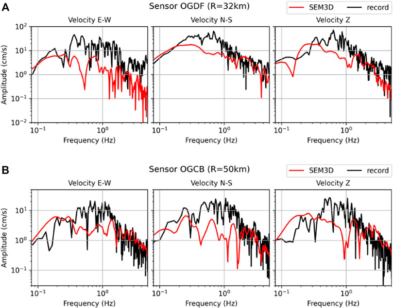
FIGURE 7. Frequency response spectra of the numerical simulation (in red) obtained with the 3D geological model and a kinematic fault model. Comparison with seismograms records (in black). Velocities are given in the East-West (E-W), North-South (N-S), and vertical (Z) directions for stations OGDF (A) and OGCB (B).

3.2 Influence of heterogeneities

Random fields were added to the 1D geological model to create small scale heterogeneities. Random fields were drawn independently in each of the three layers, thus possibly creating sharp interfaces between layers. We chose the point-source description over the kinematic fault model to limit the interactions between the source and the medium which may alter the results independently from path effects.

Figure 8 shows that introducing heterogeneities reduces the early peaks’ amplitude compared to the signals generated with the homogeneous 1D geological model. Heterogeneities also limit the duration and scale of the surface wave oscillations. This behaviour is interpreted as a consequence of the diffraction induced by heterogeneities that spread the energy content and limit the wave guide effect. Therefore, the signal obtained with a heterogeneous medium seems more realistic than those originating from the homogeneous model.

FIGURE 8

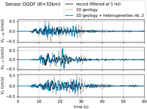
FIGURE 8. Numerical results in station OGDF obtained with a point source and the 1D geological model enhanced with random fields (blue). Comparison with the results of the homogeneous 1D geological model (grey) and the records filtered at 5 Hz (black).

However, one cannot claim that one sampling of a random field can represent the variability of all possible heterogeneities. To assess the possible impacts of heterogeneities while maintaining reasonable computational costs, two new random fields were drawn and added to the 1D geological model. Supplementary Figures S4A,B show the ground motion response in station OGDF with those random fields. One can notice that those samplings tend to increase the amplitude of the late oscillations compared to those obtained with the homogeneous medium. Therefore, the influence of random fields on the surface wave oscillations was not consistent between samplings.

Given the large variability in ground motion responses arising from the three random fields samplings, it is crucial to ensure that those responses remain physically plausible. This was done by computing the mean horizontal pseudo Spectral Acceleration (SA) in three stations for the 1D geological model and the three heterogeneous models. Then, we compared the synthetic SA with the one given by a regional Ground Motion Prediction Equation (GMPE, Berge-Thierry et al., 2003). Figure 9 shows that the synthetic SA were within the confidence bounds of the GMPE, thereby ensuring our heterogeneous models were realistic. More precisely, the first and second random field samplings were close to the GMPE. The third sampling led to SA slightly higher than the upper bound of the GMPE for stations CRU1 and OGDF. However, it is noteworthy that the record in station OGCB was also out of the confidence interval. Therefore, we had no reason to reject the third sampling based on the sole analysis of the SA.

FIGURE 9

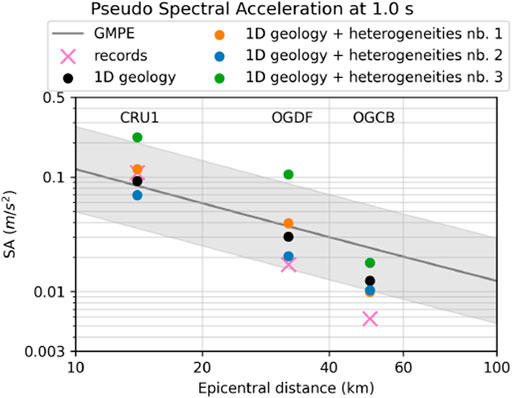
FIGURE 9. Pseudo Spectral Acceleration (SA) at 1 s in 3 stations (CRU1, OGDF, OGCB). Mean horizontal SA for records (pink cross), 1D model (black dots), 1D model with random fields (colored dots), and a GMPE (grey line) with the associated confidence interval (Berge-Thierry et al., 2003).

Moreover, Figure 9 shows that both the homogeneous 1D geology and the second sampling of the heterogeneous geology were close to the records. Although comparing the SA did not lead to a preference for one of these two models, we showed above that the heterogeneous model was able to reduce the surface wave oscillations.

As a partial conclusion, the three random fields showed a high variability that may create synthetic seismograms closer to the recorded ones, but as well, seismograms worse than those obtained with the homogeneous geological model. Therefore, a more systematic analysis of random heterogeneities involving machine learning techniques is necessary to better apprehend the relationship between heterogeneities and their impacts on ground motion.

4 Machine learning framework for dimensionality reduction

To analyze the wide range of ground motion variability created by the addition of random fields on geological models, it would be necessary study thousands of heterogeneous geological models. However, the computational cost of high-fidelity simulations makes this direct approach unaffordable. As a workaround, we propose to reduce the dimensionality of geological fields. For this purpose, we built a database of 40,000 heterogeneous S-wave velocity fields (described in Section 4.1). Then, we applied the PCA (Section 4.2) and a 3D autoencoder (Section 4.3) to this database.

4.1 Database of heterogeneous geological fields

Our database is composed of 3D heterogeneous geological fields built as 32 × 32 × 32 matrices. They can be interpreted as S-wave velocity fields on a domain of size of 9.6 km × 9.6 km × 9.6 km (illustration in Figure 11). The velocity values were chosen so as to ensure that geological fields were physically meaningful. More precisely, all samples contain a 1.8 km-thick bottom layer with constant velocity 4500 m/s. On top of this constant layer, each gelogical field was built with 1–6 layers, the number of layers and the thickness of each layer being chosen randomly. In each layer, the mean velocity was chosen according to a uniform distribution $\mathcal{U}$([1785 m/s; 3214 m/s]). In addition, a different random field was drawn in each layer, except the bottom one. The random field’s parameters were also randomly sampled. In all directions, correlation lengths were randomly chosen among {1.5, 3, 4.5, 6} km, and the coefficient of variation followed a normal distribution of mean 0.2 and standard deviation 0.1, $\mathcal{N}$(0.2, 0.1) (if a non-positive coefficient of variation was chosen, it was replaced by its absolute value). Finally, all velocities were clipped to the interval 1071–4500 m/s to ensure realistic values. It has to be noted that random fields generated this way are not stationary since their mean and standard deviation depend on the position along the z axis. The parallel generation of 40,000 geological fields took 33 min on 40 CPUs for a total size of 5.4 Gb. This dataset is publicly available at https://doi.org/10.5281/zenodo.6983054. We additionally built a similar dataset of 4000 geological fields for test purposes.

In a second stage, the database was used to study the relationship between heterogeneous geological fields and ground motion response generated by the propagation of seismic waves throughout the geological fields. For this purpose, a seismic source was placed in the constant bottom layer at coordinates (1.2 km, 1.2 km, − 8.4 km). It was parametrized as a moment tensor with the same moment, dip, rake, and slip as the Le Teil earthquake (Delouis et al., 2021). The same source time function was used with τ = 0.1. The velocity values described in the previous paragraph ensured that the numerical propagation of seismic waves was accurate up to a 5 Hz frequency (with 7 GLL points per element, each element being of size 300 m). Finally, synthetic ground motion was recorded on a 32 × 32 regular grid of virtual sensors placed at the surface.

4.2 Dimensionality reduction with PCA

To perform the PCA, 3D geological fields were considered as 1D vectors of size p = 32 × 32 × 32 = 32,768. The principal component features were computed from the sample covariance matrix S. By choosing a number of samples n = 40,000 larger than the number of features p, S was guaranteed to be of rank p (or slightly lower). Otherwise, the rank and therefore the number of principal components would have been limited by the number of samples in the database. To ease the principal components computation on the large sample covariance matrix, an incremental PCA algorithm was used (Ross et al., 2008).

Once the principal components were obtained, the PCA performances were assessed on the test database. 3D geological fields from the test database were decomposed and then reconstructed using only the k first principal components (k was of the order 500–3000). Seismic waves were then propagated throughout 1) the test geological field and 2) its corresponding reconstructed field. Errors between the two sets of surface ground motion responses were quantified with Goodness Of Fit (GOF) measures on the enveloppe and phase (Kristeková, Kristek, and Moczo 2009).

4.3 3D autoencoder with a UNet architecture

By considering geological fields as 1D vectors, the PCA loses the spatial organisation of 3D geological fields. To obtain the same reconstruction error, one may therefore expect a greater dimensionality reduction with a 3D autoencoder than a PCA. The autoencoder can be viewed as a nonlinear extension of the PCA since it creates a reduced representation of the input in what is called a latent space. The encoder associates the 3D input with the latent representation and the decoder reconstructs a 3D field from the latent representation while trying to minimize the error between the input and the reconstruction.

Our 3D autoencoder is built from the architecture of the 3D UNet developped by Wolny et al., 2020. We conducted an exhaustive search of the main hyperparameters to adapt the proposed architecture to our objectives. Our final encoder is composed of 6 blocks that increase the number of channels of the inputs from 1 to 256. As represented in Figure 10, each block is composed of two convolutional layers. Blocks are separated by max pooling layers to reduce the dimensionality from 32 × 32 × 32 to 1 × 1 × 1. A batch size of 16 was found to produce lower reconstruction errors than larger batches for both training and validation datasets.

FIGURE 10

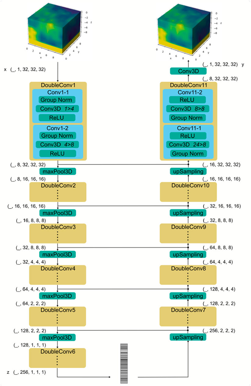
FIGURE 10. 3D UNet autoencoder with 6 blocks of double convolutions (4 million parameters in total). Skip connections between the encoder and decoder are done via concatenation.

The database of 40,000 geological fields was split in 90% of training and 10% of validation data. Inputs were centered and normalized by 4 times the standard deviation, moving values approximately into [ − 0.5, 0.5]. The training loss was simply composed of the L1 reconstruction error. The Adam optimizer was used with a learning rate of 2 ⋅ 10^–4. Training the network for 1000 epochs on 4 Nvidia Ampere A100 GPUs took 9.5 h.

5 Dimensionality reduction of complex geological fields

5.1 Assessing the reconstruction accuracy

When applying the PCA on 40,000 geological fields, 500 principal components explained 91.5% of the observed variance. This increased to 94.4% and 97.9% with respectively 1000 and 3000 components (Supplementary Figure S5). Figure 11 shows that test geological fields reconstructed with 1024 principal components are visually close to the input fields. Indeed, the heterogeneities’ size and location correspond to the inputs. However, it can be noted that geological fields reconstructed with the PCA lack some sharpness in the spatial variations and can appear blurrier than the input. This is especially visible on samples with a high coefficient of variation (e.g. last row of Figure 11). Quantitatively, the Root Mean Square Error (RMSE) was low, with a median value of 90 m/s. This corresponds to 8.6% of the minimum velocity value.

FIGURE 11

FIGURE 11. Each row represents one geological field from the test dataset of 4000 samples. (A) original field. (B) reconstruction with a PCA with 1024 principal components. (C) reconstruction with a 3D UNet autoencoder. RMSE = Root Mean Square Error.

Reconstructions obtained with the 3D UNet were also satisfying since heterogeneities were well reproduced. The median RMSE was 85 m/s, which was slightly lower than the PCA error. Interestingly, Figure 12 shows that the PCA and the 3D UNet led to very different error distributions despite having a similar median error. While the PCA reconstruction error ressembles a normal distribution, the 3D UNet histogram has larger values close to 0. This means that the 3D UNet was able to create more reconstructions with a very low error. As a counterpart, more geological fields also had a poorer reconstruction than the PCA. Among the fields showing a high reconstruction error with the 3D UNet, many had a low coefficient of variation (an example is visible on the first row of Figure 11). In those cases, the large error derived from a biased reconstruction by the neural network.

FIGURE 12

FIGURE 12. Reconstruction error on 4000 test geological fields using a PCA with 512 components (in grey) and 1024 components (in brown), and the 3D UNet (in red). (A): histogram of the error. (B): boxplot of the error, boxes extend from the 1st to the 3rd quartile, line shows the median.

When investigating the reconstruction error pixel by pixel, it appeared that on the one hand, the PCA led to a reconstruction error that was well distributed around 0. Some pixels overestimated the velocity while others underestimated it (Supplementary Figure S6A). On the other hand, the 3D UNet committed a global error on the mean velocity value leading to pixels that were all under- or over-estimated (Supplementary Figure S6B).

5.2 Influence of the dimension on ground motion response

More importantly than the reconstruction error, we were interested in the ground motion generated from reconstructed geological fields, compared to the ones generated from the input fields. Figure 13 shows GOF scores on a grid of virtual sensors at the surface. Seismic waves were propagated through a geological field with a rather large reconstruction error, around 135 m/s for both the PCA and the 3D UNet. This geological field is shown on the third row of Figure 11 and its pixel-wise reconstruction error is depicted in Supplementary Figure S6. A RMSE smaller than 135 m/s was guaranteed for 75% (resp. 72%) of the geological fields in the test database with the PCA reconstruction (resp. 3D UNet).

FIGURE 13

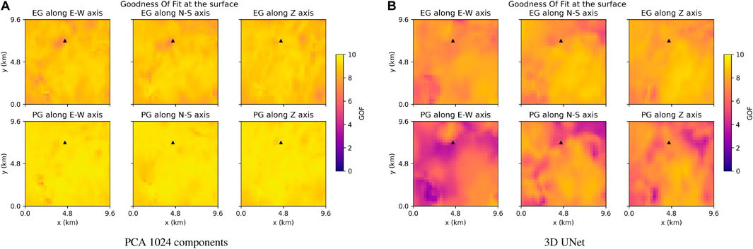
FIGURE 13. The GOFs were evaluated on the three velocity components generated by the wave propagation through a geological field reconstructed by the PCA with 1024 components (A) and the 3D UNet (B). GOF measures for each sensor on a 32×32 grid at the surface (10: perfect agreement). Each measure is given for the three velocity components: East-West (E), North-South (N), Vertical (Z) axes. EG: Enveloppe GOF, PG: Phase GOF. The black triangles show the position of the sensor in Figure 14. The corresponding V_S field is represented on the third row of Figure 11.

Figure 13 shows that a vast majority of sensors exhibit GOFs above 8, generally considered as an excellent agreement. Therefore, despite a large reconstruction error on the geological field, the surface ground motion was still very close to the reference one. One can also notice that the various types of errors described above for the PCA and the 3D UNet had very different consequences on the ground motion generated through the reconstructed geological fields. For the PCA reconstruction, the enveloppe GOFs were slightly worse than the phase GOFs. This is exemplified in Figure 14A where the signal amplitude was higher with the reconstructed field than the input one. This can be explained by the lack of small-scale heterogeneities that should have diffracted and reflected seismic waves. Signals propagated through the reconstructed geological field were therefore less attenuated than the reference ones. However, the wave arrival times were very well reproduced since the mean velocity was correctly reconstructed by the PCA.

FIGURE 14

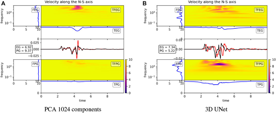
FIGURE 14. For the sensor depicted by the black triangles in Figure 13, velocity ground motion along the North-South component. Black: ground motion obtained with the input V_S field. Red: ground motion obtained with the V_S field reconstructed by (A) PCA and (B) 3D UNet. GOFs are represented in the frequency (FEG and FPG), time-frequency (TFEG and TFPG), and time (TEG and TPG) domain for the enveloppe (top) and phase (bottom).

On the contrary, ground motion responses of the geological field reconstructed by the 3D UNet differ from the input mostly in terms of phase. Since the 3D UNet underestimated (for this specific sample) the mean velocity, the reconstructed signal was delayed with respect to the reference one. However, amplitudes were well reproduced thanks to the good reconstruction of small-scale heterogeneities.

6 Discussion and conclusion

Considering the sparsity of available geological data, a 1D layered geological model was not rich enough to accurately simulate the Le Teil earthquake. Geological models can be improved by the addition of random fields that however yield a large ground motion variability. Quantitative analyses of the variability induced by heterogeneous models would require hundreds or thousands of simulations, that are computationally intractable. PCA is a common dimensionality reduction method that is well adapted to extract features from 3D random fields. However, it needed at least 1024 components in the current setting to retain good reconstruction abilities. A greater reduction could be obtained with a dedicated 3D auto-encoder architecture (3D UNet) that gave promising results.

We showed that the main ground motion characteristics of the Le Teil earthquake can be reproduced using regional geological models. The frequency response spectra were in satisfactory agreement with the recorded seismograms. However, the 1D geological model, with its peculiar subsurface layer, induced surface waves with high-amplitude oscillations. These oscillations were significantly reduced when adding random fields to the geological model, therefore leading to more realistic signals.

With the 3D geological model, surface wave oscillations disappeared. However, this model needed to be used in conjunction with the kinematic fault model to ensure that the signal energy was correctly spread over time. Otherwise, the point source model led to peak ground velocities much larger than the recorded ones. We also found some differences between ground motion generated from a point source and from an extended kinematic fault model. We interpret these differences as plausibly coming from the low depth of the Le Teil fault.

Although the addition of random fields on the 1D geological model could reduce the unrealistic surface waves oscillations, this effect was not necessarily consistent between stations and between different random fields samplings. Therefore, a larger diversity of random fields was necessary to better understand the impacts of heterogeneities on ground motion.

As a preliminary step to conduct numerical simulations on hundreds of heterogeneous geological fields, we showed that both the PCA and the 3D UNet were able to reduce the fields dimensionality while preserving their main features. With 1024 principal components, the PCA already produced geological fields with small reconstruction errors. It appeared that the PCA smoothes small scale heterogeneities, similarly to temporal signals losing their high frequency content when being decomposed by PCA. Although it did not have a major impact on the generated ground motion, the only way to alleviate this issue would be to increase the number of principal components. Since our aim is to run simulations from reduced representations of 3D random fields, this is not the path we would like to pursue. In fact, the larger the dimension, the larger the number of simulations to sample all possible heterogeneous fields, and one cannot afford running tens of thousands of high-fidelity simulations.

Different conclusions were drawn for the geological fields reconstructed by the 3D UNet. The reconstruction error was somewhat similar to the one obtained with the PCA, with more fields having an even better reconstruction. Especially, the 3D UNet was able to produce sharp outputs with small scale heterogeneities being well preserved. This mainly arises from the use of the L1 norm that favors large components during the neural network training. Although the 3D UNet produced biased reconstructions for geological fields with low coefficients of variation, this can be easily corrected by adding a regularization term to the neural network loss function. The major advantage of the 3D UNet over the PCA is its greater dimensionality reduction power. Although we acknowledge the computation power required to train the 3D UNet, the current architecture produces latent variables of size 256 which is significantly lower than the number of PCA components.

From the reduced representation of geological fields, we envision building a structured ensemble of heterogeneous geological fields. We could therefore run a limited number of high-fidelity simulations. Then thanks to the dimensionality reduction, it would be possible to exhibit a relationship between the geological field and the ground motion response. Ultimately, it may even be possible to inverse this relationship to infer real soil heterogeneities from the study of recorded ground motion.

Data availability statement

The datasets presented in this study can be found in online repositories. The names of the repository/repositories and accession number(s) can be found below: https://doi.org/10.5281/zenodo.6983054.

Author contributions

DC, FG, MB, and FL contributed to the design and implementation of the research and to the analysis of the results. FG computed the fault model. FL conducted the numerical simulations, created the database, and ran the machine learning experiments. FG and FL wrote the manuscript. All authors contributed to manuscript revision, read, and approved the submitted version.

Acknowledgments

The authors thank Clara Duverger and Pierre Arroucau for providing and explaining the geological models and Amaury Vallage for his help processing seismograms. They acknowledge the computational ressources provided by the CEA and the preliminary study of Eddy Terrasse. They are also grateful to Chiara Smerzini, Manuela Vanini, and Roberto Paolucci for the discussions on the 3D Le Teil simulations.

Conflict of interest

The authors declare that the research was conducted in the absence of any commercial or financial relationships that could be construed as a potential conflict of interest.

Publisher’s note

All claims expressed in this article are solely those of the authors and do not necessarily represent those of their affiliated organizations, or those of the publisher, the editors and the reviewers. Any product that may be evaluated in this article, or claim that may be made by its manufacturer, is not guaranteed or endorsed by the publisher.

Supplementary material

The Supplementary Material for this article can be found online at: https://www.frontiersin.org/articles/10.3389/feart.2022.1029160/full#supplementary-material

Supplementary Figure S1 | Results of the numerical simulation (in red) obtained with the 1D geological model and a point source. Comparison with seismograms records (in black) filtered at 5 Hz. Velocities are given in the East-West (E-W), North-South (N-S), and vertical (Z) directions for stations OGDF (A) and OGCB (B).

Supplementary Figure S2 | Results of the numerical simulation (in red) obtained with the 3D geological model and a point source. Comparison with seismograms records (in black) filtered at 5 Hz. Velocities are given in the East-West (E-W), North-South (N-S), and vertical (Z) directions.

Supplementary Figure S3 | Results of the numerical simulation (in red) obtained with the 3D geological model and a kinematic fault model. Comparison with seismograms records (in black) filtered at 5 Hz. Velocities are given in the East-West (E-W), North-South (N-S), and vertical (Z) directions in stations OGDF (A) and OGCB (B).

Supplementary Figure S4 | Velocities obtained with two random fields added to the 1D geological model in OGDF station. The third random field is shown in Figure 8.

Supplementary Figure S5 | Ratio of explained variance (red dots) and reconstruction computed as the L1 error (blue squares) and RMSE (cyan diamonds) as a function of the number of principal components used for the reconstruction.

Supplementary Figure S6 | Pixel-wise RMSE for one geological field reconstructed with the PCA with 1024 components (A) and the 3D UNet (B). Each image is a vertical slice parallel to the (0xz) plane with the y position specified. This sample corresponds to the third row of Figure 11.

Supplementary Table S1 | Stations with available records ordered by decreasing latitude. PGA (resp. PGV): maximum of the East-West and North-South components for the Peak Ground Acceleration (resp. Velocity). VIVF is a vertical sensor only. LDG = Geophysical and Detection Laboratory of the French Alternative Energies and Atomic Energy Commission (CEA). FR, OHP, 3C, RA are networks of RAP-R´esif (French Permanent Accelerometric Network). SNCF = French National Railway Company.

References

Arroucau, P. (2020). A preliminary three-dimensional seismological model of the crust andUppermost mantle for metropolitan franc. SIGMA2-2018-D2014. Available at: https://www.sigma-2.net/medias/files/%20sigma2-2018-d2-014-3d-velocity-model-franceapproved-public-.pdf.

Google Scholar

Berge-Thierry, C., Cotton, F., Scotti, O., Griot-Pommera, D. A., and Fukushima, Y. (2003). New empirical response spectral attenuation laws for moderate European earthquakes. J. Earthq. Eng. 7 (2), 193–222. ISSN: 1363-2469, 1559-808X. doi:10.1080/13632460309350446

CrossRef Full Text | Google Scholar

Bravard, J-P., and Gaydou, P. (2015) “Historical development and integrated management of the Rhoˆne river floodplain, from the alps to the camargue delta, France”. In: Geomorphic approaches to integrated floodplain management of lowland fluvial systems in North America and europe. New York, NY Springer , pp. 289–320. ISBN: 978- 1-4939-2379-3 978-1-4939-2380-9.Paul F. Hudson and Hans Middelkoop (visited on 08/22/2022).Available at: http://link.springer.com/10.1007/978-1-4939-2380-9_12.

CrossRef Full Text | Google Scholar

Chaljub, E. (2006). “Spectral element modeling of 3d wave propagation in the alpine valley of Grenoble, France,” in Third international symposium on the effects of surface geology on seismic motion Grenoble, France, S04, 9.

Google Scholar

Cheng, X., and Jiang, K. (2020). Crustal model in eastern qinghai-tibet plateau and western yangtze craton based on conditional variational autoencoder. Phys. Earth Planet. Interiors 309, 106584. ISSN: 00319201. doi:10.1016/j.pepi.2020.106584

CrossRef Full Text | Google Scholar

Chernov, L. A. (1960). Wave propagation in a random medium. New York: Dover publications. Translated by Richard A. Silverman. Mineola.

Google Scholar

Çiçek, Ö., Abdulkadir, A., Soeren, S. L., Brox, T., and Olaf, R., (2016) “3D U-net: Learning dense volumetric segmentation from sparse annotation”. In: Medical image computing and computer-assisted intervention – miccai 2016. 9901. Cham: Springer International Publishing, 424–432. ISBN: 978-3-319-46722- 1 978-3-319-46723-8. visited on 07/13/2022) Available at: https://link.springer.com/10.1007/978-3-319-46723-8_49.

Google Scholar

Colvez, M. (2021). Influence of the earth’s crust heterogeneities and complex fault structures on the frequency content of seismic waves. Paris-Saclay: Université Paris Saclay.

Google Scholar

De Carvalho Paludo, L. V. B., and Cottereau, R. (2019). Scalable parallel scheme for sampling of Gaussian random fields over very large domains: Parallel scheme for sampling of random fields over very large domains. Int. J. Numer. Methods Eng. 117 (8), 845–859. ISSN: 00295981. doi:10.1002/nme.5981

CrossRef Full Text | Google Scholar

De Novellis, N., Vincenzo, C., Valkaniotis, S., Casu, F., Lanari, R., Monterroso Tobar, M. F., et al. (2020). Coincident locations of rupture nucleation during the 2019 Le Teil earthquake, France and maximum stress change from local cement quarrying. Commun. Earth Environ. 1, 20. 1.1ISSN: 2662-4435. doi:10.1038/s43247-020-00021-6

CrossRef Full Text | Google Scholar

Delouis, B., Elif, O., Marine, M., Jean, P. A., Trilla, A. G., Marc, R., et al. (2021). Constraining the point source parameters of the 11 november 2019 Mw 4.9 Le Teil earthquake using multiple relocation approaches, first motion and full waveform inversions. Géoscience 353, 1–24. ISSN: 1778-7025. doi:10.5802/crgeos.78

CrossRef Full Text | Google Scholar

Dreger, , and Douglas, S. (2007). Near-fault seismic ground motions. EERC 2007-03. Berkeley: University of California. (visited on 05 02, 2022). Available at: https://citeseerx.ist.psu.edu/viewdoc/download?doi=10.1.1.434.578&rep=rep1&type=pdf.

Google Scholar

Duverger, C., Gilles, M. R., Trilla, A. G., Vallage, A., Bruno, H., and Yves, C., (2021). A decade of seismicity inMetropolitan France (2010–2019): The CEA/LDG methodologies and observations. Bull. Société Géologique Fr. 192 (1), 25.

CrossRef Full Text | Google Scholar

Faccioli, E., Maggio, F., Paolucci, R., and Quarteroni, A. (1997). 2d and 3D elastic wave propagation by a pseudo-spectral domain decomposition method”. J. Seismol. 1 (3), 237–251. ISSN: 1573-157X. doi:10.1023/A:1009758820546

CrossRef Full Text | Google Scholar

Gallovič, F. (2016). Modeling velocity recordings of the M w 6.0 South napa, California, earthquake: Unilateral event withWeak high-frequency directivity. Seismol. Res. Lett. 87 (1), 2–14. ISSN: 0895-0695, 1938-2057. doi:10.1785/0220150042

CrossRef Full Text | Google Scholar

Gangopadhyay, T., Ramanan, V., Akintayo, A., Boor, P. K., Sarkar, S., Chakravarthy, S. R., et al. (2021). 3D convolutional selective autoencoder for instability detection in combustion systems. Energy AI 4, 100067. ISSN: 26665468. doi:10.1016/j.egyai.2021.100067

CrossRef Full Text | Google Scholar

Gatti, F. (2017). Analyse physics-based de Scénarios sismiques ”de La faille Au site” : Prédiction de Mouvement sismique fort pour l’étude de Vulnérabilité sismique de Structures critiques. Paris: Université Paris Saclay. Available at: http://www.theses.fr/2017SACLC051.

Google Scholar

Gatti, F., Carvalho Paludo, L. D., Svay, A., Lopez-Caballero, F., Cottereau, R., and Clouteau, D. (2017). Investigation of the earthquake ground motion coherence in heterogeneous non- linear soil deposits. Procedia Eng. 199, 2354–2359. ISSN: 18777058. doi:10.1016/j.proeng.2017.09.232

CrossRef Full Text | Google Scholar

Gatti, F., Touhami, S., Lopez-Caballero, F., and Pitilakis, D. (2018). “3-D source-to-site numerical investigation on the earthquake ground motion coherency in heterogeneous soil deposits,” in Numerical methods in geotechnical engineering IX 9th European conference on numerical methods in geotechnical engineering. Porto (Portugal: CRC Press), 829–835. ISBN: 978-1-351-00362-9. doi:10.1201/9781351003629-104

CrossRef Full Text | Google Scholar

Haber, E. (2021). Simulation techniques benchmark, the test case of the november 11, 2019 Mw4.9 Le Teil earthquake. SIGMA2-2021-D3-082. SIGMA2.

Google Scholar

Heller, G. J. (2021). Vers Une Meilleure Estimation de La Magnitude à Partir de La Coda Sismique. Toulouse: Université Paul Sabatier.

Google Scholar

Hinton, G. E., and Salakhutdinov, R. R. (2006). Reducing the dimensionality of data with neural networks. Science 313 (5786), 504–507. ISSN: 0036-8075, 1095-9203. doi:10.1126/science.1127647

PubMed Abstract | CrossRef Full Text | Google Scholar

Hollender, F., Emeline, M., Bard, P. Y., and Ameri, G., (2018). “AreWe ready to perform fully site-specific seismic hazard studies in low–to-moderate seismicity areas?,” in Sixteenth European conference on earthquake engineering (Thessaloniki, Greece, 12.

Google Scholar

Kadeethum, T., Ballarin, F., Choi, Y., O’Malley, D., Yoon, H., and Bouklas, N. (2022). Non-intrusive reduced order modeling of natural convection in porous media using convolutional autoencoders: Comparison with linear subspace techniques. Adv. Water Resour. 160, 104098. ISSN: 03091708. doi:10.1016/j.advwatres.2021.104098

CrossRef Full Text | Google Scholar

Khazaie, S., Cottereau, R., and Clouteau, D. (2016). Influence of the spatial correlation structure of an elastic random medium on its scattering properties. J. Sound Vib. 370, 132–148. ISSN: 0022460X. doi:10.1016/j.jsv.2016.01.012

CrossRef Full Text | Google Scholar

Komatitsch, D., and Tromp, J. (1999). Introduction to the spectral element method for three-dimensional seismic wave propagation. Geophys. J. Int. 139 (3), 806–822. ISSN: 0956540X, 1365246X. doi:10.1046/j.1365-246x.1999.00967.x

CrossRef Full Text | Google Scholar

Korres, M., Lopez-Caballero, F., Alves Fernandes, V., Gatti, F., Zentner, I., Voldoire, F., et al. (2022). Enhanced seismic response prediction of critical structures via 3D regional scale physics-based earthquake simulation. J. Earthq. Eng., 1–29. ISSN: 1363-2469, 1559-808X. doi:10.1080/13632469.2021.2009061

CrossRef Full Text | Google Scholar

Kristeková, M., Kristek, J., and Moczo, P. (2009). Time-frequency misfit and goodness-of-fit criteria for quantitative comparison of time signals. Geophys. J. Int. 178 (2), 813–825. ISSN: 0956540X, 1365246X. doi:10.1111/j.1365-246X.2009.04177.x

CrossRef Full Text | Google Scholar

Ladjal, S., Newson, A., and Pham, C-H. (2019). A PCA-like autoencoder. arXiv. 1904.01277.

Google Scholar

Larroque, C., Baize, S., Julie, A., Jomard, H., Jenny, T., Godano, M., et al. (2021). Seismotectonics of southeast France: From the jura mountains to corsica. Comptes Rendus Géoscience 353 (1), 105–151. ISSN: 1778-7025. doi:10.5802/crgeos.69

CrossRef Full Text | Google Scholar

Marconato, L., Leloup, P. H., Lasserre, C., Jolivet, R., Caritg, S., Grandin, R., et al. (2022). Insights on fault reactivation during the 2019 november 11, mw 4.9 Le Teil earthquake in southeastern France, from a joint 3-D geological model and InSAR time-series analysis. Geophys. J. Int. 229 (2), 758–775. ISSN: 0956-540X, 1365-246X. doi:10.1093/gji/ggab498

CrossRef Full Text | Google Scholar

Martin, R., and Komatitsch, D. (2006). An optimized convolution-perfectly matched layer (C-pml) absorbing technique for 3D seismic wave simulation based on a finite-difference method. Geophys. Res. Abstr. 8, 03988.

Google Scholar

Maufroy, E., Chaljub, E., Hollender, F., Bard, P. Y., Kristek, J., Moczo, P., et al. (2016). 3D numerical simulation and ground motion prediction: Verification, validation and beyond – lessons from the E2VP project. Soil Dyn. Earthq. Eng. 91, 53–71. ISSN: 02677261. doi:10.1016/j.soildyn.2016.09.047

CrossRef Full Text | Google Scholar

Molinari, I., and Morelli, A. (2011). EPcrust: A reference crustal model for the European plate: EPcrust. Geophys. J. Int. 185 (1), 352–364. ISSN: 0956540X. doi:10.1111/j.1365-246X.2011.04940.x

CrossRef Full Text | Google Scholar

Ritz, J-F., Baize, S., Ferry, M., Larroque, C., Audin, L., Delouis, B., et al. (2020). Surface rupture and shallow fault reactivation during the 2019 Mw 4.9 Le Teil earthquake, France. Commun. Earth Environ. 1, 10. ISSN: 2662-4435. doi:10.1038/s43247-020-0012-z

CrossRef Full Text | Google Scholar

Ross, D. A., Lim, J., Lin, R. S., and Yang, M. H. (2008). Incremental learning for robust visual tracking”. Int. J. Comput. Vis. 77 (1), 125–141. ISSN: 1573-1405. doi:10.1007/s11263-007-0075-7

CrossRef Full Text | Google Scholar

Ruiz, J. A., Baumont, D., Bernard, P., and Berge-Thierry, C. (2011). Modelling directivity of strong GroundMotion with a fractal, K-2, kinematic source model: Modelling directivity of strong ground motion. Geophys. J. Int. 186 (1), 226–244. ISSN: 0956540X. doi:10.1111/j.1365-246X.2011.05000.x

CrossRef Full Text | Google Scholar

Scalise, M., Pitarka, A., Louie, J. N., and Smith, K. D. (2021). Effect of random 3D correlated velocity perturbations on numerical modeling of ground motion from the source physics experiment. Bull. Seismol. Soc. Am. 111 (1), 1391943–1563573. ISSN: 0037-1106. doi:10.1785/0120200160

CrossRef Full Text | Google Scholar

Shen, W., Yang, D., Xu, X., Yang, S., and Liu, S. (2022). 3D simulation of ground motion for the 2015 Mw 7.8 gorkha earthquake, Nepal, based on the spectral element method. Nat. Hazards 112, 2853–2871. ISSN: 0921-030X, 1573-0840. doi:10.1007/s11069-022-05291-1

CrossRef Full Text | Google Scholar

Shinozuka, M., and Deodatis, G. (1991). Simulation of stochastic processes by spectral representation. Appl. Mech. Rev. 44 (4), 191–204. ISSN: 0003-6900. doi:10.1115/1.3119501

CrossRef Full Text | Google Scholar

Smerzini, C., Vanini, M., Roberto, P., and Paola, T. (2022). Validation of regional physics-based ground motion scenarios: The case of the mw 4.9 2019 Le Teil earthquake in France. preprint. doi:10.21203/rs.3.rs-1552665/v1

CrossRef Full Text | Google Scholar

Stupazzini, M., Paolucci, R., and Igel, H. (2009). Near-fault earthquake ground-motion simulation in the Grenoble valley by a high-performance spectral element code. Bull. Seismol. Soc. Am. 99 (1), 286–301. ISSN: 0037-1106. doi:10.1785/0120080274

CrossRef Full Text | Google Scholar

Svay, A., Perron, V., Afifa, I., Irmela, Z., Regis, C., Clouteau, D., et al. (2017). “Spatial coherency analysis of seismic ground motions from a rock site dense array implemented during the kefalonia 2014 aftershock sequence,” in Earthquake engineering & structural dynamics (Publisher: John Wiley & Sons, Ltd 46.12), 1895–1917. ISSN: 0098-8847. doi:10.1002/eqe.2881

CrossRef Full Text | Google Scholar

Tekawade, A., Liu, Z., Peter, K., Bicer, T., Carlo, F. D., Rajkumar, K., et al. (2021). “3d autoencoders for feature extraction in X-ray tomography,” in 2021 IEEE international conference on image processing (ICIP) 2021 IEEE international conference on image processing (ICIP), 3477–3481. ISBN: 2381-8549. doi:10.1109/ICIP42928.2021.9506494

CrossRef Full Text | Google Scholar

Touhami, S., Gatti, F., Lopez-Caballero, F., Cottereau, R., de Abreu Correa, L., Aubry, L., et al. (2022). SEM3D: A 3D high-fidelity numerical earthquake simulator for broadband (0–10 Hz) seismic response prediction at a regional scale. Geosciences 12 (3), 112. ISSN: 2076-3263. doi:10.3390/geosciences12030112

CrossRef Full Text | Google Scholar

Touhami, S., Lopez-Caballero, F., and Clouteau, D. (2021). A holistic approach of numerical analysis of the geology effects on ground motion prediction: Argostoli site test. J. Seismol. 25 (1), 115–140. ISSN: 1383-4649, 1573-157X. doi:10.1007/s10950-020-09961-0

CrossRef Full Text | Google Scholar

Vallage, A., Bollinger, L., Champenois, J., Duverger, C., Trilla, A. G., Hernandez, B., et al. (2021). Multitechnology characterization of an unusual surface rupturing intraplate earthquake: The M L 5.4 2019 Le Teil event in France. Geophys. J. Int. 226 (2), 803–813. ISSN: 0956-540X, 1365-246X. doi:10.1093/gji/ggab136

CrossRef Full Text | Google Scholar

Veinante-Delhaye, A., and Santoire, J. P. (1980). “Sismicite Recente de l’Arc Sud-Armoricain et Du Nord-Ouest Du Massif Central; Mecanismes Au Foyer et Tectonique,” in Bulletin de la Société Géologique de France S7-XXII1, 93–102. ISSN: 0037-9409. doi:10.2113/gssgfbull.S7-XXII.1.93

CrossRef Full Text | Google Scholar

Vyas, J. C., Mai, P. M., Galis, M., Dunham, E. M., and Imperatori, W. (2018). Mach wave properties in the presence of source and medium heterogeneity. Geophys. J. Int. 214 (3), 2035–2052. ISSN: 0956-540X, 1365-246X. doi:10.1093/gji/ggy219

CrossRef Full Text | Google Scholar

Wolny, A., Cerrone, L., Vijayan, A., Tofanelli, R., Barro, A. V., Louveaux, M., et al. (2020). Accurate and versatile 3D segmentation of plant tissues at cellular resolution. eLife 9, e57613. ISSN: 2050-084X. doi:10.7554/eLife.57613

PubMed Abstract | CrossRef Full Text | Google Scholar

Yu, J., Zhang, L., Li, Q., Huang, W., and Sun, Z., (2021). 3D autoencoder algorithm for lithological mapping using ZY-1 02D hyperspectral imagery: A case study of liuyuan region. J. Appl. Remote Sens. 15. 04ISSN: 1931-3195. doi:10.1117/1.JRS.15.042610

CrossRef Full Text | Google Scholar

Zeng, Q., Feng, S., Brendt, W., and Lin, Y., (2021). “InversionNet3D: Efficient and scalable learning for 3D FullWaveform inversion,” in CoRR. Available at: https://arxiv.org/abs/2103.14158.

Google Scholar