Stochastic differential equation modeling of time-series mining induced ground subsidence

Mining-induced ground subsidence is a commonly observed geo-hazard that leads to loss of life, property damage, and economic disruption. Monitoring subsidence over time is essential for predicting related geo-risks and mitigating future disasters. Machine-learning algorithms have been applied to develop predictive models to quantify future ground subsidence. However, machine-learning approaches are often difficult to interpret and reproduce, as they are largely used as “black-box” functions. In contrast, stochastic differential equations offer a more reliable and interpretable solution to this problem. In this study, we propose a stochastic differential equation modeling approach to predict short-term subsidence in the temporal domain. Mining-induced time-series data collected from the Global Navigation Satellite System (GNSS) in our case study area were utilized to conduct the analysis. Here, the mining-induced time-series data collected from GNSS system regarding our case study area in Miyi County, Sichuan Province, China between June 2019 and February 2022 has been utilized to conduct the case study. The proposed approach is capable of extracting the time-dependent structure of monitored subsidence data and deriving short-term subsidence forecasts. The predictive outcome and time-path trajectories were obtained by characterizing the parameters within the stochastic differential equations. Comparative analysis against the persistent model, autoregressive model, and other improved autoregressive time-series models is conducted in this study. The computational results validate the effectiveness and accuracy of the proposed approach.

1 Introduction

Ground subsidence is a cascading geo-hazard that considerably impacts human lives and the evolution of landscapes (Gao et al., 2020a; Merghadi et al., 2020). Many factors, including earthquakes, ore mining, groundwater drought, and land-use changes, are considered to cause the widespread occurrence of ground subsidence (Gao et al., 2021; Zhou et al., 2021). Among them, mining-induced subsidence is the most impactful, as it can damage surface construction, trigger landslides, induce slope collapse, promote soil erosion, and cause other geological disasters (Diao et al., 2018; Cui et al., 2021; Li et al., 2022). Thus, a reliable approach for monitoring and predicting ground subsidence is urgently required. It will not only provide a sufficient assessment of subsidence caused damage, but also assist in mitigating the related geo-risks and potential losses.

The geo-hazard of ground subsidence and its associated risks have been studied in detail due to its destructive nature and socioeconomic impacts (Tang et al., 2021; Gao & Meguid 2022). Interferometric synthetic aperture radar (InSAR) techniques represent the mainstream approach to subsidence monitoring, and have been frequently applied to assess active ground deformation in densely populated regions. Synthetic aperture radar (SAR) sensors offer wide-range coverage and can accurately detect any surface change in a landscape (Armaş et sl. 2017; Malik et al., 2022). Galloway & Burbey (2011) summarized the advantages of using InSAR data to monitor land subsidence caused by groundwater extraction. Armas et al. (2017) utilized multi-temporal InSAR data to identify long-term ground deformation patterns and integrated them with multivariate dynamic analysis to investigate the factors that cause subsidence. Chen et al. (2018) used time-series InSAR to detect ground subsidence in regions with rapid urbanization. Diao et al. (2018) selected RadarSat-2 images acquired from InSAR to assess the geo-risk of subsidence caused by coal mining and conducted a case study in Jiulong Mine, China. He et al. (2020) integrated small baseline subset interferometry (SBAS) data with InSAR data to detect surface deformation in urban regions and assessed the impact of subsidence on buildings. InSAR is utilized for subsidence monitoring as it can simultaneously obtain the surface elevation using the phase difference of two SAR images. However, in practice, the collection of InSAR data is costly and time-consuming.

Conversely, the use of a Global Navigation Satellite System (GNSS) to detect and monitor ground subsidence can be a feasible and efficient alternative. GNSS can be applied to identify and delineate subsidence-prone areas to create a geospatial database of subsidence events or subsidence inventory (Tang et al., 2020; Gao et al., 2020b). Using GNSS technology, the temporal observation of subsidence can be obtained by sampling in up to daily intervals, based on practical needs (Eldhuset & Weydahl. 2013). Burbey (2006) proposed the use of 3D GNSS data to monitor and detect strain-induced ground subsidence. Ustun et al. (2010) applied GNSS-based temporal observations of ground subsidence to predict the landscape deformation. Monthly resolution GNSS data regarding groundwater withdrawal-induced subsidence were analyzed, and subsidence in the short term was predicted. Yuwono et al. (2019) used both D-InSAR and GNSS to obtain time-series data to analyze ground subsidence in coastal regions. The GNSS dataset collected from a base station in the case study area was analyzed, and the subsidence rate was computed. Hinderer et al. (2020) combined InSAR, GNSS, gravity, and precise leveling datasets to generate a comprehensive spatial–temporal dataset for modeling the ground subsidence process. Shahbazi et al. (2022) integrated InSAR and GNSS datasets to perform a multivariate analysis of hydrogeological factors that induced ground subsidence. Daily time-series subsidence data were acquired and utilized to assess future subsidence in both spatial and temporal domains.

In recent years, machine-learning and statistical modeling approaches are becoming popular in analyzing time-series GNSS dataset. Lee & Park (2013) applied classification and regression tree (CART) and random forest to predict the coal-mining induced subsidence in the temporal domain. The factors that impact the speed of subsidence are analyzed according to their importance. Abdollahi et al. (2019) trained a support vector machine (SVM) to predict the water-induced ground subsidence in the temporal domain which considered drawdown and other influential factors. Taravatrooy et al. (2018) integrated k-mean clustering with several machine-learning algorithms to predict the time-series subsidence values and the prediction performance has been further optimized. Rafie et al. (2020) combined fuzzy inference system with artificial neural networks (ANN) to predict the time-series ground subsidence. Based on their work, Ranjgar et al. (2021) proposed using gray wolf optimization (GWO) to optimize the adaptive neuro-fuzzy inference system to obtain higher prediction accuracy in terms of time-series subsidence prediction. Overall, all machine-learning algorithms have achieved promising results in predicting short-term subsidence in the near future. However, one major shortcoming of using machine learning algorithms is that they all lack sufficient interpretability. They are all serving as “black-box” functions which does not provide any information to the field engineers except the predictive outcome (Petch & Nelson 2021).

In this study, instead of applying machine-learning algorithms, we propose using a stochastic differential equation (SDE) to model time-series subsidence in the temporal domain. The proposed approach produced short-term predictions of subsidence using historic subsidence data and provided point estimates of future subsidence values in the short term. Moreover, it offers plausible time-path trajectories of the land deformation process with interpretability, which contributes to the feasibility of the onsite application of the proposed approach. The parameters that characterize the SDE for each site can be interpreted easily with sufficient intuition. This makes formulating a model that can be extended depending on the specific data patterns for each GNSS monitoring site easy. To validate the usefulness of the SDE model, field data collected from an ore mining site in Miyi County, Sichuan Province, China, were utilized in this study. Time-series data collected via a GNSS were utilized to develop and validate the SDE models. To evaluate the performance of the proposed SDE approach, three-point estimation-related evaluation criteria was computed. A comparative analysis with traditional time-series models was also conducted in this study.

This paper has the following major contributions:

• It proposes a novel approach developing SDE models to fit and predict the subsidence time-series.

• The fitted models with explicit fitted parameters increased the interpretability and reproducibility in terms of applying the SDE onsite.

The rest of the manuscript is organized as follows: Section 2 describes the theoretical foundation of SDEs and the process of estimating model parameters. Section 3 introduces the basic specifications of the ore mining site that was taken as the case study area. Section 4 presents the computational results and a comparative analysis. Finally, Section 5 concludes the paper and provides future research directions.

2 Methodology

2.1 Stochastic differential equation

A stochastic differential equation (SDE) is a differential equation containing one or multiple stochastic components that can be used to derive a solution (Iversen et al., 2016). SDEs are usually selected to model systems with large random components, such as those in quantitative finance (Rukanda et al., 2022), meteorology (Palmer 2019), and environmental science (Li 2022a; Li 2022b).

The modeling process of an SDE typically consists of model structure selection, parameter estimation, predictive modeling, and prediction evaluation (Bjerregård et al., 2022). In this research, all the aforementioned steps were performed for short-term prediction of land subsidence. A generic SDE describing the evolution of state variable $X_t$ is stated as Eq. 1:

$d{X}_{\mathit{t}}=f\left(X_t,U_t,t\right)dt+g\left(X_t,t\right)d{W}_t,(1)$

where $f\left(\bullet \right)$ denotes the drift term that depicts the long-term trend, $g\left(\bullet \right)$ is the diffusion term that describes short-term stochasticity, $U_t$ denotes the vector of inputs, and $W_t$ is a standard Wiener process. In practice, more than one state variable is often necessary; thus, a set of SDEs is formulated in that case. Here, the system dynamics are conveniently described in continuous time as a set of SDEs, whereas the data are available in discrete time (Bjerregård et al., 2022).

However, Eq. 1 is not well defined in some cases, as the derivatives of $d{W}_t$ may not exist. Thus, the integral equation in Eq. 2 is a better representation of the evolution of the state variable.

$X_{\mathit{t}}=X_{\mathbf{0}}+\underset{0}{\overset{t}{{\displaystyle \int }}}f\left(X_s,U_s,s\right)\mathrm{d}s+\underset{0}{\overset{t}{{\displaystyle \int }}}g\left(X_s,s\right)\mathrm{d}{W}_s,(2)$

where the second term $\underset{0}{\overset{t}{{\displaystyle \int }}}g\left(X_s,s\right)\mathrm{d}{W}_s$ can be derived using Ito’s lemma. Therefore, with drift defined as $f\left(X_t,U_t,t\right)$ and the diffusion coefficient as $g\left(X_t,t\right)$, we can obtain the density function $j\left(x,t\right)$ (see Eq. 3) of the random variable $X_t$ in state $x$ at time $t$, which is the solution for the SDE in Eq. 1 (Björk 2009). We have

$\frac{\partial }{\partial t}j\left(x,t\right)=-\frac{\partial }{\partial x}\left[f\left(x,t\right)j\left(x,t\right)\right]+\frac{{\partial }^2}{\partial x^2}\left[D\left(x,t\right)j\left(x,t\right)\right],(3)$

which is known as the Fokker–Planck equation or the Kolmogorov forward equation.

2.2 Stochastic differential equation for subsidence prediction

In this study, the ground subsidence system was complex and constantly changing over time. The monitored subsidence data were collected at different discrete time stamps. Hence, we defined the observed subsidence $Y_k$ at time $t_k$ as a measurement based on the state function $h\left(\bullet \right)$. The entire system can be defined in Eqs 4–6:

$d{X}_t={\theta }_x\left(p_t{\mu }_x-X_t\right)dt+{\sigma }_x{X}_t^{{\beta }_x}d{W}_x,(4)$

$d{U}_t={\theta }_u\left({\mu }_u-U_t\right)dt+{\sigma }_{u}d{W}_u,(5)$

$Y_{\mathit{t}}=h\left(X_{t_k},t_k\right)+e_k,(6)$

where $p_t$ denotes the numerical instant subsidence prediction at time $t$, ${\mu }_x$ is the local scaling factor for each GNSS monitoring site, ${\theta }_x$ is a constant over time that governs how rapidly the model returns to the predicted subsidence, $e_k$ is the measurement error, where $e_k\sim N\left(0,{\sigma }^2\right)$, ${\sigma }_x$ characterizes the system white noise, and $h\left(\bullet \right)$ has specific forms depending on the specific modeling task. In this study, we define $h\left(X_{t_k},t_k\right)=X_{t_k}$ and ${\theta }_x$ as constantly positive, which produces a stochastic process that is governed predominantly by past observations of ground subsidence at the same location (Li et al., 2021a; Li et al., 2021b).

In addition, the point forecast provided by the aforementioned SDE model systematically shifts in time with respect to the prediction horizons, which is 1 h in this study. Determining the appropriate input size $t_k$ for the model is critical for achieving a sufficient prediction performance (Satyarthee et al., 2013). Here, the autocorrelation function (ACF) was computed to capture the temporal dependency structure among the monitored ground subsidence datasets. The ACF can be computed using Eq. 7 as follows:

${ACF}_{T,h}=\frac{{{\displaystyle \sum }}_{t=1}^{T-h}\left(Y_t-\overline{Y}\right)\left(Y_{t+h}-\overline{Y}\right)}{{{\displaystyle \sum }}_{t=1}^T{\left(Y_t-\overline{Y}\right)}^2},(7)$

where $Y_t$ is the observed subsidence at time $t$; and $\overline{Y}$ is the mean of the historic observations within the time period of length $T$.

To select statistically significant historic lags, the Ljung–Box statistic is considered a reliable threshold for screening all historic lags based on their ACF values (Tang et al., 2022). The Ljung–Box statistic was computed using Eq. 8, as follows:

$Q_H=T\left(T+2\right){\displaystyle \sum }_{h=1}^H{\left(T-h\right)}^{-1}{ACF}_{T,h}^2,(8)$

where $Q_H$ is the computed Ljung–Box statistic, which follows an asymptotic chi-square distribution, and $H$ is the selected arbitrary value that the related literature suggested, based on many empirical studies.

2.3 Parameter estimation

To estimate the optimal parameter settings of the SDE for ground subsidence prediction, maximization of the approximated likelihood was conducted. To satisfy the conditions on $f\left(\bullet \right)$ and $g\left(\bullet \right)$ according to Eq. 1, the approximated likelihood function can be expressed in Eq. 9 as follows:

$L\left(\theta ;y_N\right)=\left({\displaystyle \prod }_{k=1}^N\frac{\exp \left(-1/2{ϵ}_k^{\top }{R}_{\left(k|k-1\right)}^{-1}{ϵ}_k\right)}{\sqrt{\mathrm{d}\mathrm{e}\mathrm{t}\left(R_{\left(k|k-1\right)}\right)}{\left(\sqrt{2\pi }\right)}^l}\right)p\left(Y_0|\theta \right),(9)$

where $l$ is the dimension of the samples; $N$ denotes the number of observations; ${\left(\bullet \right)}^{\top }$ denotes the vector transpose; ${ϵ}_k$ denotes the white noise; $R_{\left(k|k-1\right)}$ denotes the conditional variance of the prediction by SDE; and $p\left(Y_0|\theta \right)$ represents the likelihood of seeing observation $Y_0$. To optimize the SDE parameter setting, we targeted the log-likelihood function, as expressed in Eq. 10:

$\log \left(L\left(\theta ;\left(y_N|Y_0\right)\right)\right)=-\frac{1}{2}{\displaystyle \sum }_{k=1}^N\left(\log \left(\mathrm{d}\mathrm{e}\mathrm{t}\left(R_{\left(k|k-1\right)}\right)\right)+{ϵ}_k^{\top }{R}_{\left(k|k-1\right)}^{-1}{ϵ}_k\right)-\log \left(2\pi \right)\frac{Nl}{2},(10)$

where $\theta$ represents the parameter setting within the predictive SDE.

2.4 Prediction performance evaluation criterion

Once the SDEs are fitted with the optimal parameters derived via the maximum likelihood estimation, the prediction outcome should be assessed using the performance evaluation criterion. Because we are performing point-based prediction for short-term subsidence, three commonly utilized evaluation criteria, including mean absolute error (MAE), mean absolute percentage error (MAPE), and root mean square error (RMSE), were applied in this study (Li 2022a).

First, MAE (Deng et al., 2022) was utilized to measure the absolute difference between the measured subsidence and predicted subsidence. This can be computed using Eq. 11.

$\mathrm{M}\mathrm{A}\mathrm{E}=\frac{{{\displaystyle \sum }}_{=\mathbf{1}}^N\left|Y_{\mathit{t}}-{\widehat{Y}}_{\mathit{t}}\right|}{N},(11)$

where $N$ denotes the total number of observations, $Y_{\mathit{t}}$ represents the actual subsidence, and ${\widehat{Y}}_{\mathit{t}}$ denotes the predicted subsidence. It measures the absolute errors between the actual subsidence and corresponding predictions.

Second, the MAPE (Li 2022a; Deng et al., 2022) computes the errors in terms of percentage with respect to the actual measurement. The MAPE can be computed using Eq. 12:

$\mathrm{M}\mathrm{A}\mathrm{P}\mathrm{E}=\frac{1}{N}{\displaystyle \sum }_{i=1}^N\left|\frac{Y_t-{\widehat{Y}}_t}{Y_t}\right|\ast 100\%,(12)$

where $N$ denotes the total number of data samples; $Y_{\mathit{t}}$ represents the actual subsidence; and ${\widehat{Y}}_{\mathit{t}}$ denotes the predicted subsidence. It measures the proportion of prediction errors with respect to the actual measured subsidence.

Third, RMSE (Li 2022b) measures the average squared error and is sensitive to outliers in the test dataset. The formula used to compute the RMSE is expressed in Eq. 13.

$\mathrm{R}\mathrm{M}\mathrm{S}\mathrm{E}=\sqrt{\frac{{{\displaystyle \sum }}_{i=\mathbf{1}}^N{\left(Y_t-{\widehat{Y}}_t\right)}^{\mathbf{2}}}{N}}.(13)$

where $N$ denotes the total number of data samples; $Y_{\mathit{t}}$ represents the actual subsidence; and ${\widehat{Y}}_{\mathit{t}}$ denotes the predicted subsidence. It measures the squared errors which is more sensitive to the outliers when measuring the prediction performance.

2.5 Traditional parametric prediction models

To demonstrate the accuracy and effectiveness of the proposed approach, three traditional parametric predictive models, namely, the persistence model, autoregressive (AR) model, autoregressive with extra input (ARX) model, and generalized autoregressive conditional heteroskedasticity (ARX-GARCH) model, were selected for comparative analysis.

The persistence model is an AR (1) model with Gaussian noise, which can be expressed as

${\widehat{Y}}_t=Y_{t-1}+{ϵ}_t,(14)$

where ${ϵ}_t$ denotes the Gaussian noise (white noise) and it follows ${ϵ}_t\sim N\left(0,{\sigma }^2\right)$.

The AR model can be expressed as follows:

${\widehat{Y}}_t={\psi }_0+{\displaystyle \sum }_{i=1}^p{\psi }_i{Y}_{t-i}+{ϵ}_t,(15)$

where ${\psi }_0$ and ${\psi }_i$ denote the intercept and coefficient between the current observation and the historic lags in the subsidence time series, respectively (Li 2022b).

In comparison with AR, the ARX contains the truncated Gaussian noise ${ϵ}_t$, which follows a Gaussian distribution truncated at ${-(\psi }_0+{{\displaystyle \sum }}_{i=1}^p{\psi }_i{Y}_{t-i}+\varphi p_t)$. The ARX model can be expressed as

${\widehat{Y}}_t={\psi }_0+{\displaystyle \sum }_{i=1}^p{\psi }_i{Y}_{t-i}+\varphi p_t+{ϵ}_t.(16)$

The ARX-GARCH model is an improved ARX model with the same truncated Gaussian noise ${ϵ}_t$. However, the estimated variance has a different formulation. The prediction and variance are expressed in Eqs 17, 18, respectively:

${\widehat{Y}}_t={\psi }_0+{\displaystyle \sum }_{i=1}^p{\psi }_i{Y}_{t-i}+\varphi p_t+{ϵ}_t,(17)$

${\sigma }_k^2={\alpha }_0+{\displaystyle \sum }_{i=1}^p{\alpha }_i{\sigma }_{i-1}^2+{{\displaystyle \sum }_{j=1}^q{\beta }_iϵ}_{t-i},(18)$

where ${\alpha }_i$ and ${\beta }_i$ are both the fitted coefficients for historic variance and noise. The estimated variance as expressed in Eq. 18 can be perceived as a linear combination of historic variance as well as the historic noise.

3 Dataset summary

In this study, field data were collected from our case study location, which is an ore mining site located in Miyi County, Sichuan Province, China. Data collection was conducted via a GNSS with multiple sensors configured over the subsidence region to obtain a full-scale estimate of the land deformation process. Eight GNSS-based sensors are displayed, and the configuration is shown in Figure 1.

FIGURE 1

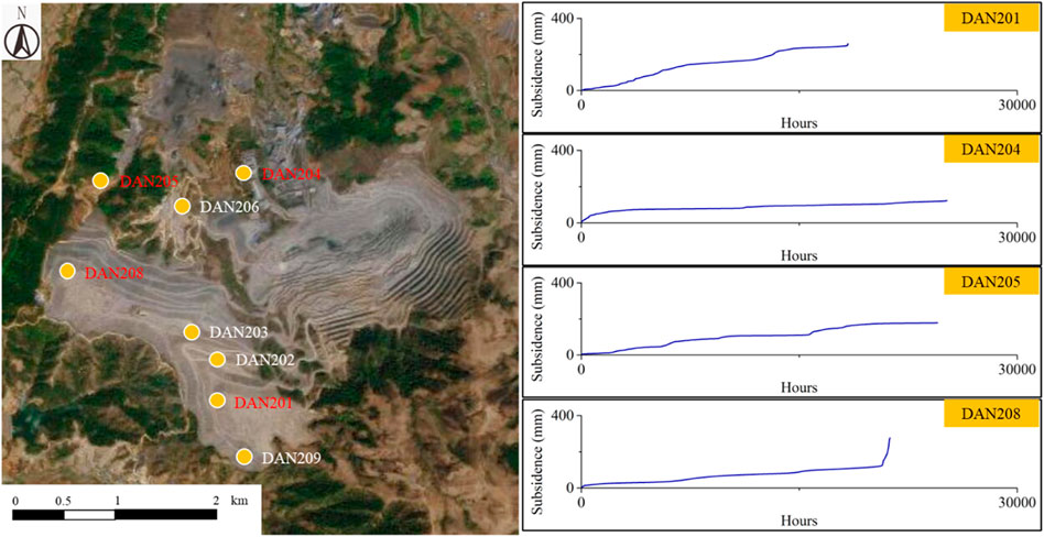
FIGURE 1. Configuration of GNSS monitoring points in the case study area.

Data collection using GNSS was initiated in June 2019 after a significant ground subsidence event caused by ore mining. At each GNSS monitoring point, data were collected in hourly intervals. The unit for monitoring the subsidence process is millimeters, and the cumulative subsidence is visualized on the right side of Figure 1. As the hourly rate of ground deformation is too slow and inconvenient for computation, we merged the dataset on a daily basis and computed the daily instant subsidence from the original collected cumulative data. The daily instant subsidence was computed through time-series differencing, which subtracts the previous observation from the current observation. The differenced time-series of subsidence indicates the daily instant rate of ground subsidence which is more valuable for monitoring the underlying geo-hazard. A summary of the time series data collected from the eight monitoring sites is presented in Table 1.

TABLE 1

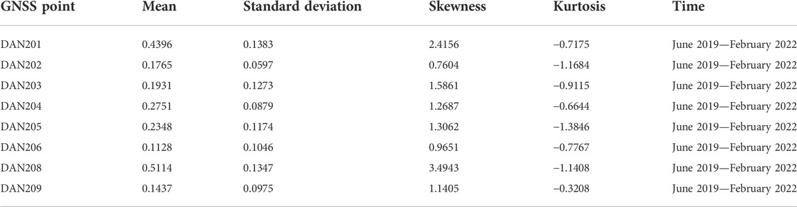
TABLE 1. Summary of the daily instant subsidence monitoring dataset.

As can be seen in Table 1, the mean, standard deviation, skewness, and kurtosis for all eight GNSS monitoring sites for daily subsidence were calculated. Four monitoring points (i.e., DAN201, DAN204, DAN205, and DAN208) can be observed to have higher average daily changes than the other four points. Thus, they were selected as representative points for this study.

4 Experimental results

To predict daily subsidence in the short term, experiments were conducted to determine the input size and train the SDE model to accurately predict short-term instant subsidence. The ACFs (see Eq. 7) are first computed to capture the temporal dependency structure of the subsidence time-series data. The results for the ACFs at the four selected GNSS monitoring sites are shown in Figure 2.

FIGURE 2

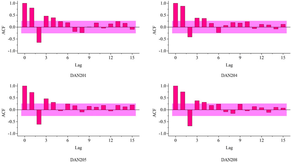
FIGURE 2. ACFs and the threshold based on Ljung–Box statistic.

As can be observed in Figure 2, we computed the ACFs for all lags between lag-0 (current subsidence) and lag-15, which denotes the historic instant subsidence 15 days ago. The values of ACF vary between -1 and 1, whereas the Ljung–Box statistics (see Eq. 8) are visualized as the boundaries of the pink region. Any lags with an ACF value larger than the Ljung–Box statistic (i.e., outside of the pink region) are considered to have a significant statistical correlation with the current instant subsidence series. All four monitoring points displayed similar patterns; the first four lags were statistically significant and were thus selected to train the SDE models for the next step.

In this study, each of the four monitoring points (DAN201, DAN204, DAN205, and DAN208) developed one SDE, and the training was performed independently. The parameters for each SDE were estimated by maximizing the log-likelihood function, as expressed in Eq. 10 in Section 2.3. Once the value converges, the optimal parameter setting is achieved, as summarized in Table 2.

TABLE 2

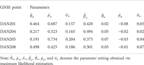
TABLE 2. Parameters obtained via maximum likelihood estimation.

Table 2 provides the estimation of the SDE parameters at the four selected GNSS monitoring points. The values of the log-likelihood function, which denote the values after convergence, are also presented. Using these obtained parameters, we developed SDEs to perform 1-day ahead subsidence prediction and 12-day ahead prediction simultaneously.

In the 1-day ahead subsidence prediction task, we used subsidence data of 24 consecutive days as the training–validation dataset and the following 1-day subsidence as the test dataset. Nested cross-validation was performed based on data from 24 consecutive days and the test was performed independently. The training, validation, and test data for the four GNSS monitoring sites are shown in Figure 3.

FIGURE 3

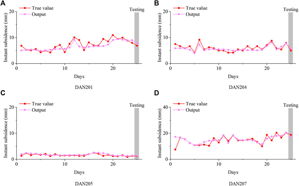
FIGURE 3. 1-day ahead prediction of instantaneous subsidence. (A) DAN201, (B) DAN204, (C) DAN205, (D) DAN207.

Figure 3 displays the training, validation, and test processes for the instant subsidence series in the 1-day ahead prediction task. The parameters for the SDE models were estimated using the maximum likelihood estimation. Three performance evaluation criteria, including the MAE (see Eq. 11), and MAPE (Eq. 12), and RMSE (Eq. 13) were computed and are summarized in Table 3.

TABLE 3

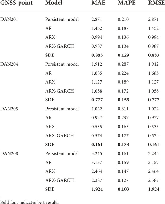
TABLE 3. Summary of 1-day ahead prediction performance.

In Table 3, the SDE produces the smallest values across all selected GNSS points with respect to all evaluation criterions. This demonstrates its superiority in performing short-term subsidence prediction tasks. Meanwhile, the persistent model produces the highest error rates and it confirms its inferiority in capturing the temporal patterns within the subsidence dataset.

A 12-day ahead prediction of instant subsidence was also performed for each GNSS monitoring site. Here, the subsidence data from the previous consecutive 60 days were selected as the training/validation dataset, and the subsidence measured in the following 12 days was selected as the test dataset. The training, validation, and test performance for the 12-day ahead prediction task is shown in Figure 4. In addition, the performance evaluation criteria, including the MAE (see Eq. 11), and MAPE (Eq. 12), and MSE (Eq. 13) were computed and are summarized in Table 4.

FIGURE 4

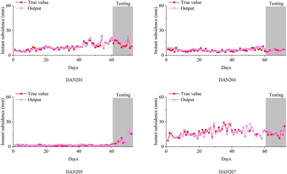
FIGURE 4. 12-day ahead prediction of instantaneous subsidence.

TABLE 4

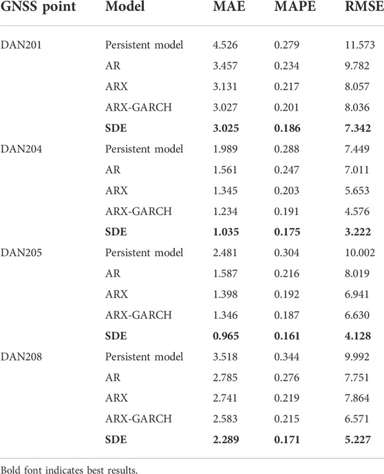
TABLE 4. Summary of 12-day ahead prediction performance.

According to Table 4, the SDE model provides the top prediction performance in 12-day ahead subsidence prediction tasks using the data collected from four selected GNSS monitoring points. It produces the smallest MAE, MAPE, and also RMSE which outperforms the traditional time-series models and thus validated its superiority in capturing time dependence structure within the time-series subsidence dataset.

Finally, to provide a visual comparison of the prediction performance, Figure 5 summarizes all evaluation criteria across the four selected GNSS sites. In both the 1-day ahead prediction and 12-day ahead prediction tasks, DAN205 had the smallest errors with respect to all criteria. This can be attributed mainly to the stationarity of the measured incidence at this site. In comparison, site DAN208 produced the highest prediction errors for both tasks. This phenomenon is due to the large variance and fast rate of measured instant subsidence. Table 1 confirms that the DAN208 data contains a large mean daily subsidence, large variance, high skewness, and high kurtosis. All basic statistics indicate the non-stationarity of the data collected from DAN208, and thus the existence of more challenges in developing accurate predictive SDE models.

FIGURE 5

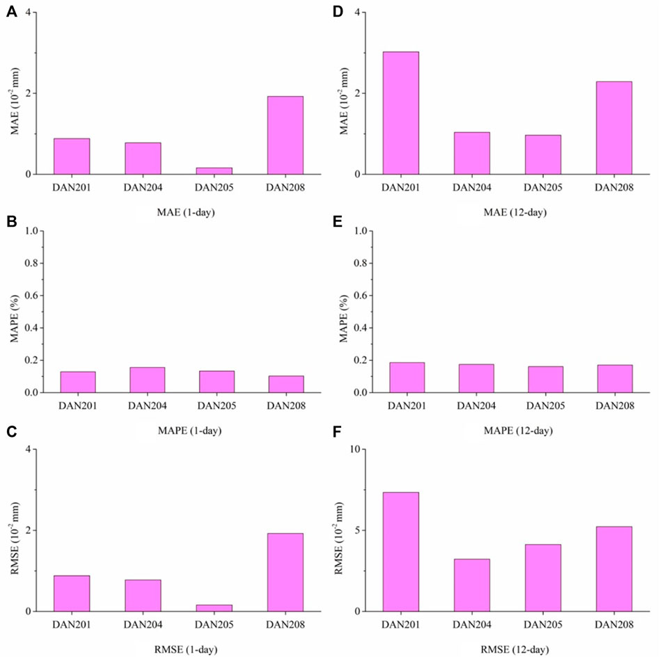
FIGURE 5. Summary of all evaluation metrics across the selected GNSS points.

5 Discussion

This research proposed using SDE models to train and forecast instant surface subsidence. Currently, the mainstream of other related research all selected machine-learning models to tackle this task. In comparison, the main advantages of the SDE model can be summarized into the following two aspects: First, the SDE model has higher interpretability. As introduction in Section 2, the SDE model is a parametric model where the engineers can directly observe the fitted parameters. Comparatively, the machine-learning models are “black-box” function which nobody is aware of the inside functions. Second, the SDE model has higher reproducibility. Since SDE model is also a data-driven model, the engineers can always get the same model by fitting the model over the same dataset. However, in comparison, machine-learning models have lower reproducibility. A lot of factors including random initialization, parameter setting, as well as hardware quality all impact the overall training process. Thus, no machine-learning models would reproduce the exact same results.

On the other hand, the main disadvantage of the SDE model as well as other parametric models, which were selected for comparative analysis in this study, is also obvious. All the parametric models have limited capacity in handling highly nonlinear patterns in the temporal domain. As a contrast, the machine-learning models such as artificial neural networks, can always overfit the training dataset by simply adding more hidden layers and hidden nodes. Thus, the SDE can be underfitting in complex tasks compared with machine-learning models respectively.

6 Conclusion

In this study, GNSS technology was applied to monitor mining-induced surface subsidence in the temporal domain. A stochastic differential equation was established to forecast short-term subsidence and capture the data-driven time-dependent structure. Three key measurement metrics—MAE, MAPE, and RMSE—were selected to evaluate the performance of the point estimate of short-term subsidence. A comparative analysis against the persistent, AR, ARX, and ARX-GARCH models was performed using the same dataset collected from the case study area.

For hazard early warning, it is important to mitigate the risk of casualties and property loss. Computational results revealed that a stochastic differential equation model is an accurate and effective approach. In comparison with traditional parametric models, stochastic differential equations provide higher interpretability and reproducibility.

Data availability statement

The raw data supporting the conclusion of this article will be made available by the authors, without undue reservation.

Author contributions

WG, LT, and NP contributed to the conception of the study; SM and XL carried out in-site investigation; WG, SM, and XL performed the computational study; WG, XL, and XC performed the data analyses and wrote the manuscript.

Funding

This research is supported by the Opening fund of Major Hazard Measurement and Control Key Laboratory of Sichuan Province, China (Grant No. KFKT-2022-01).

Conflict of interest

The authors declare that the research was conducted in the absence of any commercial or financial relationships that could be construed as a potential conflict of interest.

Publisher’s note

All claims expressed in this article are solely those of the authors and do not necessarily represent those of their affiliated organizations, or those of the publisher, the editors and the reviewers. Any product that may be evaluated in this article, or claim that may be made by its manufacturer, is not guaranteed or endorsed by the publisher.

References

Abdollahi, S., Pourghasemi, H. R., Ghanbarian, G. A., and Safaeian, R. (2019). Prioritization of effective factors in the occurrence of land subsidence and its susceptibility mapping using an SVM model and their different kernel functions. Bull. Eng. Geol. Environ. 78 (6), 4017–4034. doi:10.1007/s10064-018-1403-6

CrossRef Full Text | Google Scholar

Armaş, I., Mendes, D. A., Popa, R. G., Gheorghe, M., and Popovici, D. (2017). Long-term ground deformation patterns of bucharest using multi-temporal InSAR and multivariate dynamic analyses: A possible transpressional system? Sci. Rep. 7 (1), 43762–43813. doi:10.1038/srep43762

PubMed Abstract | CrossRef Full Text | Google Scholar

Bjerregård, M. B., Møller, J. K., Brok, N. B., Madsen, H., and Christiansen, L. E. (2022). Probabilistic forecasting of rainfall response in a Danish stormwater tunnel. J. Hydrology 612, doi:127956doi:10.1016/j.jhydrol.2022.127956

CrossRef Full Text | Google Scholar

Björk, T. (2009). Arbitrage theory in continuous time. Oxford University Press.Oxford, UK

Google Scholar

Burbey, T. J. (2006). Three-dimensional deformation and strain induced by municipal pumping, Part 2: Numerical analysis. J. Hydrology 330 (3-4), 422–434. doi:10.1016/j.jhydrol.2006.03.035

CrossRef Full Text | Google Scholar

Chen, G., Zhang, Y., Zeng, R., Yang, Z., Chen, X., Zhao, F., et al. (2018). Detection of land subsidence associated with land creation and rapid urbanization in the Chinese loess plateau using time series insar: A case study of lanzhou new district. Remote Sens. 10 (2), 270. doi:10.3390/rs10020270

CrossRef Full Text | Google Scholar

Cui, S., Pei, X., Jiang, Y., Wang, G., Fan, X., Yang, Q., et al. (2021). Liquefaction within a bedding fault: Understanding the initiation and movement of the Daguangbao landslide triggered by the 2008 Wenchuan Earthquake (Ms = 8.0). Eng. Geol. 295, 106455. doi:10.1016/j.enggeo.2021.106455

CrossRef Full Text | Google Scholar

Deng, J., Zeng, T., Yuan, S., Fan, H., and Xiang, W. (2022). Interval prediction of building foundation settlement using kernel extreme learning machine. Front. Earth Sci. (Lausanne). 10, 939772. doi:10.3389/feart.2022.939772

CrossRef Full Text | Google Scholar

Diao, X., Bai, Z., Wu, K., Zhou, D., and Li, Z. (2018). Assessment of mining-induced damage to structures using InSAR time series analysis: A case study of Jiulong mine, China. Environ. Earth Sci. 77 (5), 166–214. doi:10.1007/s12665-018-7353-2

CrossRef Full Text | Google Scholar

Eldhuset, K., and Weydahl, D. J. (2013). Using stereo SAR and InSAR by combining the COSMO-SkyMed and the TanDEM-X mission satellites for estimation of absolute height. Int. J. Remote Sens. 34 (23), 8463–8474. doi:10.1080/01431161.2013.843808

CrossRef Full Text | Google Scholar

Galloway, D. L., and Burbey, T. J. (2011). Review: Regional land subsidence accompanying groundwater extraction. Hydrogeol. J. 19, 1459–1486. doi:10.1007/s10040-011-0775-5

CrossRef Full Text | Google Scholar

Gao, G., Meguid, M. A., and Chouinard, L. E. (2020a). On the role of pre-existing discontinuities on the micromechanical behavior of confined rock samples: A numerical study. Acta Geotech. 15 (12), 3483–3510. doi:10.1007/s11440-020-01037-0

CrossRef Full Text | Google Scholar

Gao, G., Meguid, M. A., Chouinard, L. E., and Xu, C. (2020b). Insights into the transport and fragmentation characteristics of earthquake-induced rock avalanche: Numerical study. Int. J. Geomech. 20 (9), 4020157. doi:10.1061/(asce)gm.1943-5622.0001800

CrossRef Full Text | Google Scholar

Gao, G., Meguid, M. A., Chouinard, L. E., and Zhan, W. (2021). Dynamic disintegration processes accompanying transport of an earthquake-induced landslide. Landslides 18, 909–933. doi:10.1007/s10346-020-01508-1

CrossRef Full Text | Google Scholar

Gao, G., and Meguid, M. A. (2022). Microscale characterization of fracture growth in increasingly jointed rock samples. Rock Mech. Rock Eng. 55, 6033–6061. doi:10.1007/s00603-022-02965-x

CrossRef Full Text | Google Scholar

He, Y., Wang, W., Yan, H., Zhang, L., Chen, Y., and Yang, S. (2020). Characteristics of surface deformation in lanzhou with sentinel-1A TOPS. Geosciences 10 (3), 99. doi:10.3390/geosciences10030099

CrossRef Full Text | Google Scholar

Hinderer, J., Saadat, A., Cheraghi, H., Bernard, J. D., Djamour, Y., Amighpey, M., and Tavakoli, F. (2020). “Water depletion and land subsidence in Iran using gravity, GNSS, InSAR and precise levelling data,” in International association of geodesy symposia (Berlin, Heidelberg: Springer). doi:10.1007/1345_2020_125

CrossRef Full Text | Google Scholar

Iversen, E. B., Morales, J. M., Møller, J. K., and Madsen, H. (2016). Short-term probabilistic forecasting of wind speed using stochastic differential equations. Int. J. Forecast. 32 (3), 981–990. doi:10.1016/j.ijforecast.2015.03.001

CrossRef Full Text | Google Scholar

Lee, S., and Park, I. (2013). Application of decision tree model for the ground subsidence hazard mapping near abandoned underground coal mines. J. Environ. Manag. 127, 166–176. doi:10.1016/j.jenvman.2013.04.010

PubMed Abstract | CrossRef Full Text | Google Scholar

Li, H., Deng, J., Feng, P., Pu, C., Arachchige, D., and Cheng, Q. (2021). Short-term Nacelle orientation forecasting using bilinear transformation and ICEEMDAN Framework. Front. Energy Res. 9, 780928. doi:10.3389/fenrg.2021.780928

CrossRef Full Text | Google Scholar

Li, H., Deng, J., Yuan, S., Feng, P., and Arachchige, D. (2021). Monitoring and identifying wind turbine generator bearing faults using deep belief network and EWMA control charts. Front. Energy Res. 9, 799039. doi:10.3389/fenrg.2021.799039

CrossRef Full Text | Google Scholar

Li, H., He, Y., Xu, Q., Deng, j., Li, W., and Wei, Y. (2022). Detection and segmentation of loess landslides via satellite images: A two-phase framework. Landslides 19, 673–686. doi:10.1007/s10346-021-01789-0

CrossRef Full Text | Google Scholar

Li, H. (2022). SCADA data-based wind power interval prediction using LUBE-based deep residual networks. Front. Energy Res. 10, 920837. doi:10.3389/fenrg.2022.920837

CrossRef Full Text | Google Scholar

Li, H. (2022). Short-term wind power prediction via spatial temporal analysis and deep residual networks. Front. Energy Res. 10, 920407. doi:10.3389/fenrg.2022.920407

CrossRef Full Text | Google Scholar

Malik, K., Kumar, D., Perissin, D., and Pradhan, B. (2022). Estimation of ground subsidence of New Delhi, India using PS-InSAR technique and Multi-sensor Radar data. Adv. Space Res. 69 (4), 1863–1882. doi:10.1016/j.asr.2021.08.032

CrossRef Full Text | Google Scholar

Merghadi, A., Yunus, A. P., Dou, J., Whiteley, J., ThaiPham, B., Bui, D. T., et al. (2020). Machine learning methods for landslide susceptibility studies: A comparative overview of algorithm performance. Earth-Science Rev. 207, 103225. doi:10.1016/j.earscirev.2020.103225

CrossRef Full Text | Google Scholar

Palmer, T. N. (2019). Stochastic weather and climate models. Nat. Rev. Phys. 1 (7), 463–471. doi:10.1038/s42254-019-0062-2

CrossRef Full Text | Google Scholar

Petch, J., Di, S., and Nelson, W. (2021). Opening the black box: The promise and limitations of explainable machine learning in cardiology. Can. J. Cardiol. 38, 204–213. doi:10.1016/j.cjca.2021.09.004

PubMed Abstract | CrossRef Full Text | Google Scholar

Rafie, M., and Namin, F. S. (2015). Prediction of subsidence risk by FMEA using artificial neural network and fuzzy inference system. Int. J. Min. Sci. Technol. 25 (4), 655–663. doi:10.1016/j.ijmst.2015.05.021

CrossRef Full Text | Google Scholar

Ranjgar, B., Razavi-Termeh, S. V., Foroughnia, F., Sadeghi-Niaraki, A., and Perissin, D. (2021). Land subsidence susceptibility mapping using persistent scatterer sar interferometry technique and optimized hybrid machine learning algorithms. Remote Sens. 13 (7), 1326. doi:10.3390/rs13071326

CrossRef Full Text | Google Scholar

Rukanda, G. S., Govinder, K. S., and O'Hara, J. G. (2022). Option pricing: The reduced-form SDE model. J. Differ. Equations Appl. 28 (4), 590–604. doi:10.1080/10236198.2022.2055472

CrossRef Full Text | Google Scholar

Satyarthee, G. D., Pankaj, D., and Sharma, B. S. (2013). Rabbit Ear” scalp deformity caused by massive subdural effusion in infant following bilateral burr-hole drainage. J. Pediatr. Neurosci. 8 (3), 235. doi:10.4103/1817-1745.123690

PubMed Abstract | CrossRef Full Text | Google Scholar

Shahbazi, S., Mousavi, Z., and Rezaei, A. (2022). Constraints on the hydrogeological properties and land subsidence through GNSS and InSAR measurements and well data in Salmas plain, northwest of Urmia Lake, Iran. Hydrogeol. J. 30 (2), 533–555. doi:10.1007/s10040-021-02416-x

CrossRef Full Text | Google Scholar

Tang, P., Chen, G. Q., Huang, R. Q., and Wang, D. (2021). Effect of the number of coplanar rock bridges on the shear strength and stability of slopes with the same discontinuity persistence. Bull. Eng. Geol. Environ. 80 (5), 3675–3691. doi:10.1007/s10064-021-02180-y

CrossRef Full Text | Google Scholar

Tang, P., Chen, G. Q., Huang, R. Q., and Zhu, J. (2020). Brittle failure of rockslides linked to the rock bridge length effect. Landslides 17 (4), 793–803. doi:10.1007/s10346-019-01323-3

CrossRef Full Text | Google Scholar

Tang, Y., Deng, J., Zang, C., and Wu, Q. (2022). Chaotic modeling of stream nitrate concentration and transportation via IFPA-ESN and turning point analyses. Front. Environ. Sci. 10, 855694. doi:10.3389/fenvs.2022.855694

CrossRef Full Text | Google Scholar

Taravatrooy, N., Nikoo, M. R., Sadegh, M., and Parvinnia, M. (2018). A hybrid clustering-fusion methodology for land subsidence estimation. Nat. Hazards (Dordr). 94 (2), 905–926. doi:10.1007/s11069-018-3431-8

CrossRef Full Text | Google Scholar

Ustun, A., Tusat, E., and Yalvac, S. (2010). Preliminary results of land subsidence monitoring project in Konya Closed Basin between 2006–2009 by means of GNSS observations. Nat. Hazards Earth Syst. Sci. 10 (6), 1151–1157. doi:10.5194/nhess-10-1151-2010

CrossRef Full Text | Google Scholar

Yuwono, B. D., Awaluddin, M., and ., N. (2019). Land subsidence monitoring 2016-2018 analysis using GNSS CORS UDIP and DinSAR in semarang. KnE Eng. 4 (3), 95–105. doi:10.18502/keg.v4i3.5832

CrossRef Full Text | Google Scholar

Zhou, J., Wei, J., Yang, T., Zhang, P., Liu, F., and Chen, J. (2021). Seepage channel development in the crown pillar: Insights from induced microseismicity. Int. J. Rock Mech. Min. Sci. 145, 104851. doi:10.1016/j.ijrmms.2021.104851

CrossRef Full Text | Google Scholar