Characterizing the shallow structure with the multimodal dispersion curves and the body wave refraction traveltimes from deep seismic sounding data

Deep seismic sounding (DSS) profiles are one of the most powerful tools for detecting crustal structures, and they have been deployed worldwide. Generally, the analysis of DSS data mainly focuses on body waves, while the surface waves are considered noise. We suggest that the surface waves in DSS data can be used to constrain subsurface structures. In this study, we use a DSS profile in the Piedmont and Atlantic Coastal Plain as an example to present the usage of the DSS surface wave. Multimodal dispersion curves were extracted from the DSS data with the Frequency-Bessel transform method, and were used in Monte Carlo joint inversions with body wave refraction traveltimes to constrain the shallow structures. Through the inversion, a horizontal stratum on the surface was identified in the Piedmont, and a two-layer sedimentary structure was identified in the Atlantic Coastal Plain. Comparisons with existing studies verified the accuracy of the shallow structures obtained in this study, demonstrating that the shallow velocity structure could be well constrained with the additional constraints provided by the multimodal dispersion curves. Thus, we believe that further research on the surface waves recorded in DSS surveys is warranted.

1 Introduction

Deep seismic sounding profiles (abbreviated as DSS, also known as active source seismic wide-angle reflection/refraction profiles) are an important tool for interpreting crustal and lithospheric structures (Chen et al., 2017). With seismic wide-angle reflections and refractions, DSS profiles can obtain deep crustal and lithospheric velocity structures with little prior information. A large number of DSS profiles have been constructed to study crustal and lithospheric structures worldwide (e.g., Kosminskaya, 1971; Pakiser & Mooney, 1989; Benz et al., 1992; Mooney et al., 1998; Li et al., 2006; Hübscher & Gohl, 2014; Duan et al., 2016; Lin et al., 2019; Marzen et al., 2019; Guo e al., 2019; Zhao & Guo et al., 2019), and their results were collected to build global crustal models (e.g., CRUST 5.1 presented by Mooney et al., 1998) and regional crustal models (e.g., HBCrust 1.0 presented by Duan et al., 2016; Lin et al., 2019). These models have been used to solve a wide range of both seismological and nonseismological problems (Mooney et al., 1998).

Generally, the P-wave phases and surface waves are clear in most DSS datasets, and they are therefore easy to identify; in contrast, the S-wave phases are relatively difficult to identify. The P-and S-wave phases from the deep crust (e. g. refractions Pn and Sn from the uppermost mantle, and the reflections PmP and SmS from Moho) are mainly used to constrain the middle-lower crust and the uppermost mantle structure, while the P-and S-wave refractions (Pg and Sg) from the basement are used to constrain the upper crustal structure. However, surface waves are always considered coherent noise. In shallow/near-surface geophysics, surface wave analysis is a powerful and widely used tool for detecting subsurface structures (e.g., Socco & Strobbia, 2004; Lu and Zhang, 2006; Park et al., 2007; Maraschini and Foti, 2010). Thus, we suggest that surface waves in DSS data could also be used to constrain shallow/near-surface structures. With the additional information from the surface wave, a finer shallow structure (approximately 0–2 km depth) can be constrained by the DSS data, and it will be helpful for the many studies, such as estimating site response (Schleicher & Pratt, 2021), earthquake ground motion simulation (Fischer et al., 1995; Frankel et al., 2009), receiver function analysis (Zheng et al., 2005; Li et al., 2017; Anggono et al., 2018) and tectonic evolution research (Lawrence & Hoffman, 1993a; Marzen et al., 2020).

In this study, we extracted multimodal dispersion curves from the onshore DSS line in the Atlantic Coastal Plain (ACP) with the Frequency-Bessel transform (F-J) method, and then we performed the joint inversion of the multimodal dispersion curves and the Pg and Sg travel times to constrain the shallow structure. A thin layer in the Piedmont and a two-layer sediment structure in the ACP were identified with the additional constraints provided by the dispersion curves, demonstrating that surface wave analysis is helpful when imaging a higher resolution shallow structure for DSS datasets.

2 Data and methods

2.1 The data

From 2014 to 2015, onshore and offshore seismic surveys were conducted by the Eastern North American Margin Community Seismic Experiment (ENAM-CSE) project, which was funded by NSF-GeoPRISMS. The profiles extended from the eastern Piedmont to the Atlantic Ocean and yielded high quality data (P- and S-body waves and surface waves from both active sources and earthquakes) (Lynner et al., 2020). The seismic line used in this study is the north onshore ENAM-CSE seismic line (Line one in Figure 1). Line one is a 220 km-long seismic line located in Virginia and North Carolina, consisting of five borehole explosions (182 kg bulk emulsion in each borehole) and 708 vertical component seismographs (4.5 Hz Geospace GS11D instruments). The spacing between the western two shots (SP11 and SP12) is approximately 70 km, and the spacing between the other shots is approximately 30 km. The seismograph spacing is approximately 320 m. Both P- and S-body waves and surface waves are visible on the seismic record sections (Figure 2; Guo et al., 2019).

FIGURE 1

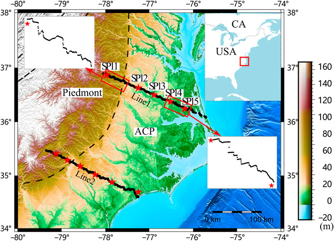
FIGURE 1. Geometry of the ENAM-CSE onshore seismic lines. The black dashed lines represent the geological terrane boundaries, and the red stars represent explosion sources. The black dots represent the seismographs. ACP denotes the Atlantic Coastal Plain. The detailed views in the figure show the crooked-line geometries.

FIGURE 2

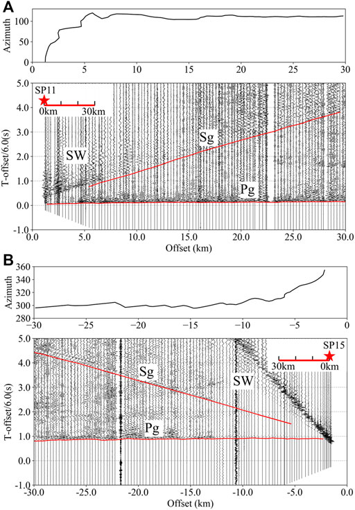
FIGURE 2. Azimuths of the source-receiver raypaths and seismic record sections plotted at a reduction velocity of 6.0 km/s. In the upper right corner of the seismic record sections, the red stars represent the sources, and the seismic record sections are recorded by the seismographs on the red line. Pg and Sg are the P- and S-wave refractions respectively, and the picked traveltimes are marked by the red lines. SW represents the surface wave. (A) Azimuths of the SP11 source-receiver raypaths and the corresponding seismic record section. (B) Azimuths of the SP15 source-receiver raypaths and the corresponding seismic record section.

Although the acquisition geometry for the ENAM DSS Line one is not straight (Figure 1), the azimuths of the source-receiver raypaths (Figure 2) show that the crooked seismic line could be considered a straight line after ∼10 km offset. The seismic line near the source is very crooked, indicating that it is better to treat the velocity structure as laterally homogeneous when we process the seismic data near the sources (Zelt, 1999).

2.2 The conventional DSS data processing method

The seismic record section in the DSS data (Figure 2) is the shot gather plotted with the reduction velocity ($V_{\mathrm{r}\mathrm{e}\mathrm{d}}$). The y-axis of the seismic record section map is the reduced time ($T_{\mathrm{r}\mathrm{e}\mathrm{d}}$) calculated by the $V_{\mathrm{r}\mathrm{e}\mathrm{d}}$and real time:

$T_{\mathit{r}\mathit{e}\mathit{d}}=t-off\mathit{s}\mathit{e}\mathit{t}/V_{\mathit{r}\mathit{e}\mathit{d}.}(1)$

With the seismic record sections, we could identify and manually pick the traveltimes according to the characteristics of each seismic phase (Braile and Smith, 1975; Giese et al., 1976). As the first arrivals, the Pg traveltimes are very easy to pick, and then the Sg traveltimes can be picked under the guidance of picked Pg traveltimes (Musacchio et al., 1997). The uncertainties of the picked traveltimes could be evaluated by the signal-to-noise ratio (SNR) of the seismic data (Zelt and Forsyth 1994).

After picking the traveltimes from each shot gather, 1D models are constructed using the traveltimes and the corresponding amplitudes with little prior information (Braile and Smith, 1975; Giese et al., 1976). Then, an initial 2D model along the seismic line is constructed by combining the 1D models, and the preferred 2D model is obtained by the inversion of all the body wave traveltimes.

Because of the large DSS source spacing and the receiver spacing, minimum-structure models should be applied in the 1D/2D model constructions to avoid overinterpreting the data (Constable et al., 1987; Zelt, 1999). The desirability of the minimum-structure model is the principle of Occam’s razor: the velocity structure should be as simple, or as smooth as possible to reduce the temptation to overinterpret the data (Constable et al., 1987; Zelt, 1999). To characterize the subsurface structure including the velocity layers with large velocity contrast (e.g., the sediment structure in this study), the minimum-structure model is usually the simplest layered models fitting the DSS data. $x^2$ is usually set as the misfit function for minimum-structure model inversions (Zelt & Smith, 1992; Zelt & Barton, 1998; Zelt, 1999) and is expressed as follows:

$x^2=\frac{1}{n}{\displaystyle \sum }_i{{[(t}_i^o-t_i^s)/e_i]}^2(2)$

where $t_i^o$ represents the ith value of the observed body traveltimes, $t_i^s$ represents the ith value of the calculated body traveltimes, and $e_i$ is the uncertainty of the value $t_i^o$. $n$ is the number of picked traveltimes. ${\mathrm{x}}^2=0$ represents that the fitting errors are equal to 0, and${\mathrm{x}}^2=1$ represents that the fitting errors are equal to the uncertainties of the picked data, indicating that the corresponding model has already satisfied the data (Bevington, 1969; Zelt, 1999).

2.3 Analysis methods for the surface wave

2.3.1 The F-J method for multimodal dispersion curves extraction

The F-J method is an array-based surface wave analysis method designed for extracting multimodal dispersion curves from ambient noise cross-correlation functions (Wang et al., 2019). Li & Chen (2020) extended this method to the application of earthquake records when the azimuth range is controlled within 90°, which could also be used for active source seismic records. The multimodal dispersion curves obtained by this method has been used in the imaging of many shallow/near-surface structures (Wu et al., 2019; Yang et al., 2019;Li et al., 2020) and deep structures (Wu et al., 2020; Zhan et al., 2020; Sun et al., 2021).

A simple formula is used in the F-J method to retrieve the dispersion spectrum ($I\left(c,\omega \right)$) from Green’s function ($C\left(r,\omega \right)$) and is expressed as follows:

$I\left(c,\omega \right)=\int {C\left(r,\omega \right)J}_0\left(kr\right)rdr,(3)$

where $J_0\left(kr\right)$ is the 0^th-order Bessel function of the first type. k represents the wavenumber, r is the distance between the receiver and the source, c denotes the velocity, and $\omega$is the frequency. The surface wave dispersion curves can be identified by the maximum of $I\left(c,\omega \right)$. For the observed seismic data, $C\left(r,\omega \right)$ is the seismic trace with offset $r$, so a seismic array is needed to calculate $I\left(c,\omega \right)$ , and the dispersion curves identified from $I\left(c,\omega \right)$ are associated with the average structure beneath the seismic array.

Recently, the F-J method has been improved to include the multiwindow scanning (MWS) method (Li & Chen, 2020; Li et al., 2021a, b) and modified frequency-Bessel transform (MFJ) method (Li et al., 2021b; Xi et al., 2021; Zhou & Chen, 2021). In the MWS method, time windows calculated by the surface wave group velocity are applied on the seismic traces to improve the SNR of the F-J spectrum ($I\left(c,\omega \right)$), and additional modes can be resolved by the MWS method (Li & Chen, 2020). In the MFJ method, the Bessel function $J_0\left(kr\right)$ is replaced by the Hankel function, and some of the crossed artifacts in the F-J spectrum can be removed (Xi et al., 2021; Zhou & Chen, 2021). In this study, both the MWS and MFJ methods were applied to extract the dispersion curves from the DSS data.

2.3.2 The inversion scheme

Since Pg, Sg and the surface waves are visible in the ACP DSS data, we suggest that the joint inversion of body wave refraction traveltimes and dispersion curves should be performed to constrain the shallow structure. In addition, to ensure that our inversion scheme can be conveniently applied to most of the existing DSS data, the inversion scheme with surface waves should be as close as possible to the inversion scheme of conventional DSS data processing. We first use all seismic data (multimodal dispersion curves, Pg and Sg travel times) in each shot gather to construct 1D models, and then construct the 2D model by using the interpolation of these 1D models.

In this study, the Monte Carlo inversion method (Socco and Boiero, 2008; Maraschini and Foti, 2010.) was used to construct 1D models with the extracted dispersion curves and Pg and Sg traveltimes. In the Monte Carlo inversion, generous random initial models were generated to perform the model parameter space sampling, and the preferred models were selected according to the acceptance criterion from the initial models. The acceptance criterion of the Monte Carlo method for the joint inversion of Pg and Sg traveltimes and multimodal dispersion curves is as follows:

$x_p^2\le 1\&x_s^2\le 1\&x_{\mathit{d}\mathit{i}\mathit{s}}^2\le 1,(4)$

where $x_p^2$ , $x_s^2$ and $x_{\mathrm{d}\mathrm{i}\mathrm{s}}^2$are the ${\mathrm{x}}^2$ of Pg, Sg and the multimodal dispersion curves respectively.

The ${\mathrm{x}}^2$ of Pg and Sg are calculated by Eq. 2. The calculation of the multimodal dispersion curves $x_{\mathrm{d}\mathrm{i}\mathrm{s}}^2$ should avoid the errors caused by associating a picked dispersion curve with an incorrect mode number (Maraschini et al., 2010). To solve this problem, we calculated the errors between a picked dispersion curve and each of the calculated multimodal dispersion curves, and then the picked dispersion curve was associated with the calculated dispersion curve corresponding to minimum error. The error between the jth picked dispersion curve and the kth calculated multimodal dispersion curves is calculated as follows:

$f_{jk}=\frac{1}{n_j}{\displaystyle \sum }_i{{[(V}_{ij}^o-V_{ik}^s)/e_{ij}]}^2(5)$

where $f_{jk}$ denotes the error between the jth picked dispersion curve and the kth calculated dispersion curve, and $n_j$ is the number of values in the jth picked dispersion curve.; $V_{ij}^o$ and $V_{ik}^s$ are the ith values in the jth picked modal dispersion curve and the kth calculated modal dispersion curve respectively, and $e_{ij}$ is the uncertainty of the picked value $V_{ij}^o$.

The jth picked dispersion curve is associated with the calculated dispersion curve corresponding to minimum error, so the fitting error $x_j$of the jth picked dispersion curve is as follows:

$x_j=\min \left(f_{j1},f_{j2},\dots ,f_{jk}\right).(6)$

The ${\chi }_{\mathrm{d}\mathrm{i}\mathrm{s}}^2$ of the picked multimodal dispersion curves is the average fitting error of all picked dispersion curves, and is expressed as follows:

$x_{\mathit{d}\mathit{i}\mathit{s}}^2=\frac{1}{m}{\displaystyle \sum }_j{x}_j,(7)$

where m is the number of picked dispersion curves.

3 Results

3.1 Multimodal dispersion curves extracted from the DSS data

To implement the F-J method on the DSS data, we should transform the seismic traces from the time domain $C\left(r,t\right)$ to the frequency domain $C\left(r,\omega \right)$ using Fourier transform. With $C\left(r,\omega \right)$ observed in different traces ($r$s), $I\left(c,\omega \right)$ can be numerically integrated by Eq. 3, and then, the F-J spectrogram is plotted with $I\left(c,\omega \right)$ to pick dispersion curves and corresponding uncertainties. For each shot gather, we first divided the seismic line to 30 km-long segments, which is equal to the shot source spacing, to extract the dispersion curves. Then, the multimodal dispersion curves were extracted from the shorter segments to increase the lateral resolution of the inversion result.

3.1.1 Multimodal dispersion curves extracted from the 30-km-long seismic record sections

Figure 3 shows the F-J spectrograms extracted from the 0–30 km offset seismic record section of SP11 and SP15 with the MFJ and MWS methods. Two dispersion curves are visible in the spectrograms of SP11 (Figures 3A,B). The higher modal dispersion curve is not clear in the MFJ spectrogram (Figure 3A), but it can be greatly enhanced by the MWS method (Figure 3B). Three dispersion curves are visible in all of the spectrograms of SP15 (Figures 3C,D). It is noteworthy that a vertical signal (marked by the ellipse in Figure 3C) exists in the spectrogram extracted by the MFJ method. Compared with the F-J spectrogram obtained by the original F-J method (Supplementary Figure S6A), this vertical signal is attenuated by the MWS method (Figure 3D) but enhanced by the MFJ method (Figure 3C), so it is difficult to determine whether this vertical signal is a dispersion curve or an artifact. We ignore this confusing “vertical signal” for now and will discuss whether it is a dispersion curve using the inversion results.

FIGURE 3

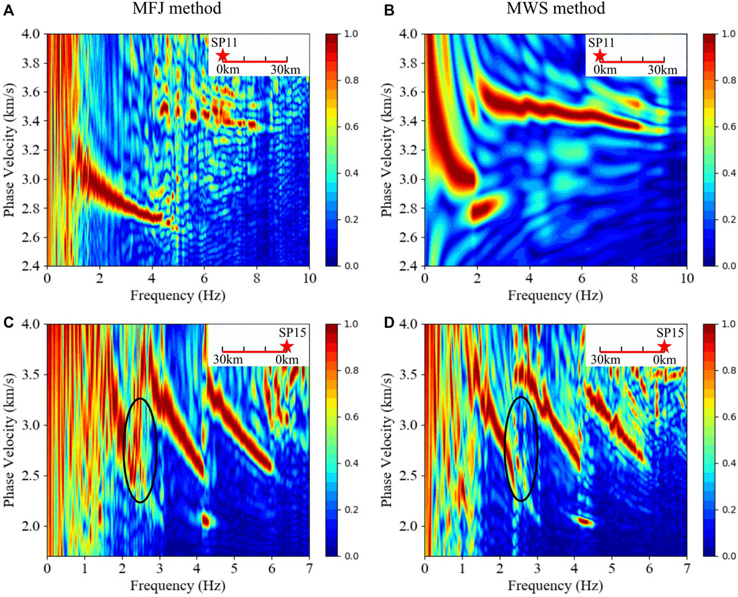
FIGURE 3. F–J spectrograms extracted from 30-km-long seismic record sections. In the upper right corner of each figure, the red star represents the source, and the F-J spectrogram is extracted from the seismic data on the red line. (A) and (B) are the spectrograms extracted from the SP11 data with the MFJ method and MWS method, respectively. (C) and (D) are the spectrograms extracted from the SP15 data with the MFJ method and MWS method, respectively.

The dispersion curves are picked from the overtones of the F-J spectrograms, and the uncertainties of the dispersion curves are set to the widths of the red overtones in the F-J spectrograms (Figure 4). Because of the “vertical signal”, it is difficult to associate the picked dispersion curves with correct mode numbers. Thus, the picked dispersion curves are named mode 1, mode 2, and mode three for convenience.

FIGURE 4

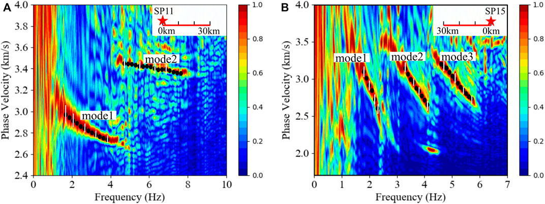
FIGURE 4. The multimodal dispersion curves picked from the F-J spectrograms. The black dots are the picked dispersion curves. The white vertical lines are the uncertainties of the picked dispersion curves. In the upper right corner of each figure, the stars represent the sources, and the F-J spectrograms are extracted from seismic data on the red lines. (A) The multimodal dispersion curves picked from the 0–30 km offset seismic record section of SP11. (B) The multimodal dispersion curves picked from the 0–30 km offset seismic record section of SP15.

3.1.2 Multimodal dispersion curves extracted from the 10-km-long seismic record sections

We successfully extracted F-J spectrograms from the 10-km-long seismic record sections (Figure 5). For the F-J spectrograms extracted from the 10-km-long SP11 data (Figures 5A–C), the overtones are nearly located in the same place, indicating the subsurface structure within 30 km offset of SP11 is nearly laterally homogenous. For the F-J spectrograms extracted from the 10-km-long SP15 data (Figures 5D–F), the variation in the overtones suggests that the phase wave velocities gradually increase from the 0 km offset to the 30 km offset of SP15.

FIGURE 5

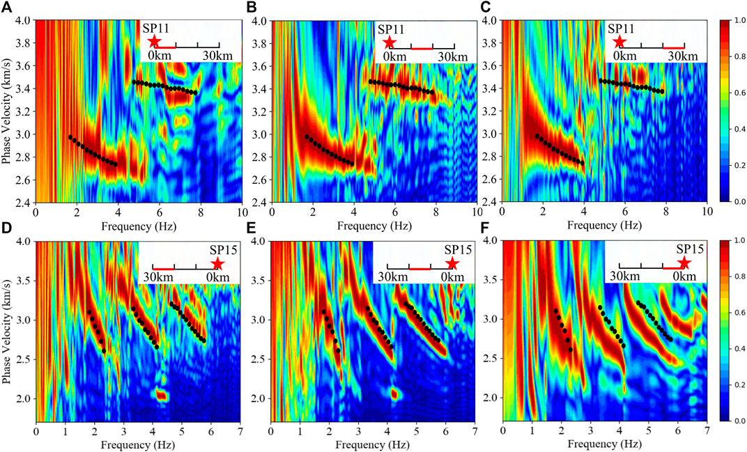
FIGURE 5. F–J spectrograms extracted from the 10-km-long seismic record sections. In the upper right corner of each figure, the stars represent the sources, and the F-J spectrograms are extracted from seismic data on the red lines. The black dots in (a)–(c) are the dispersion curves picked from the 30-km-long SP11 F-J spectrograms (Figure 4A), and the black dots in (D–F) are the dispersion curves picked from the 30-km-long SP15 F-J spectrograms (Figure 4B). (A–C) are the F-J spectrograms extracted from the 0–10 km offset, 10–20 km offset, and 20–30 km offset of SP11, respectively. (D–F) are the F-J spectrograms extracted from the 20–30 km offset, 10–20 km offset, and 0–10 km offset of SP15, respectively.

Overall, we applied the F-J method to the seismic data of the ENAM Line1, and multimodal dispersion curves could be successfully obtained within a 30 km offset of SP11 and between SP14 and SP15. The shortest segment that can be used to extract dispersion curves is approximately 10 km. However, dispersion curves cannot be obtained from the seismic data between SP12 and SP14. Guo et al. (2019) showed that the jump of refractions, the disappearance of refractions and very curved refractions are visible in the seismic record section between SP12 and SP14, suggesting a large lateral variation in the shallow structure between SP12 and SP14. Generally, in array-based surface wave analyses such as the F-J method, the obtained dispersion curves are regarded as an average effect of the structure beneath the array, so we inferred that the failure of applying the F-J method to the seismic data between SP12 and SP14 may be related to the complex shallow structure.

3.2 The inversion results

To obtain the minimum-structure 1D model, we first used two-layer models to perform the inversion. If the inversion failed, the three-layer models were used to perform the inversion instead.

3.2.1 The velocity models constrained by the 30-km-long seismic record section from SP11

Two-layer models were successfully used to perform the joint inversion of the multimodal dispersion curves and the Pg and Sg traveltimes from seismic data within a 30 km offset of SP11. The model spacing for the Monte Carlo inversion included 3 parameters: Vs.1 and Vs.2 denoting the S-wave velocities of the first and second layers respectively, and T1 denoting the thickness of the first layer. The P-wave velocities were calculated by Vs.1 and Vs.2 with the empirical Vp-Vs relation (Brocher, 2005) during the inversion. The upper and lower limits of Vs.1, Vs.2 and T1 were 0.5–3.5 km/s, 3.0–3.8 km/s and 0.2–3 km (shown as the green lines in Figure 6B), respectively. A total of 10⁶ two-layer models were randomly generated in the model space, and nine models (Figure 6B; Table 1) were accepted by the acceptance criterion of the joint inversion (Eq. 4). In the model space, the accepted models (Figure 6B) were concentrated in a very small range, indicating that high resolution shallow structure was constrained by the inversion.

FIGURE 6

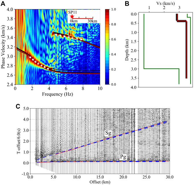
FIGURE 6. The results of the joint Monte Carlo inversion with the multimodal dispersion curves and the Pg and Sg travel times from the SP11 seismic data. (A) The black lines are the calculated dispersion curves of the accepted models, the red lines are the calculated dispersion curves of the best fitting model, and the white dots are the picked dispersion curves. In the upper right corner, the red star represents the source, and the F-J spectrogram is extracted from the seismic data on the red line. (B) The black lines are the accepted models, and the red line is the best fitting model. The green lines are the boundaries of the model parameters, and 10⁶ initial two-layer models were randomly generated between the green lines. (C) The red lines are the picked Pg and Sg, and the blue dashed lines are the calculated Pg and Sg of the accepted models.

TABLE 1

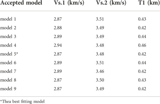
TABLE 1. The models fitting the SP11 seismic data.

3.2.2 The velocity models constrained by the 30-km-long seismic record section from SP15

According to a previous study on body wave arrivals (Guo et al., 2019), the average Vp/Vs. ratio of the ACP sediment may be much lower than the empirical value calculated by Brocher (2005), indicating that the Vp/Vs. ratio should be introduced as a variable in the inversion of the SP15 seismic data. A total of 10⁶ two-layer models were randomly generated to perform the Monte Carlo inversion, but none of the models were accepted by the acceptance criterion (Eq. 4), so the three-layer models were used to perform the inversion.

Based on the prior information provided by the DSS body wave traveltimes analysis (Guo et al., 2019), the bottom layer (third layer) of the three-layer models was set as the basement, and the corresponding P- and S-wave velocities were 6.0 km/s and 3.5 km/s, respectively. There are six model parameters in the model space: Vs.1 and Vs.2 denoting the S-wave velocities of the first two layers, the corresponding Vp1/Vs.1 ratio and Vp2/Vs.2 ratio and thicknesses T1 and T2. The upper and lower limits of the model parameters were set as follows: 0.5–3.0 km/s for Vs.1, 0.5–3.49 km/s for Vs.2, 1.1–5.0 for both Vp1/Vs.1 and Vp2/Vs.2 and 0.two to two km for both T1 and T2. In addition, the sum of the first two layer thicknesses was less than 3 km.

Seven models were selected from the 10⁶ initial three-layer models according to the acceptance criterion (Eq. 4). The dispersion curves of the accepted models are very different from each other, so we plotted them separately in Figure 7. All of the accepted model parameters are shown in Table 2 and Figure 8, and the best fitting model is model 4 (Figure 8B).

FIGURE 7

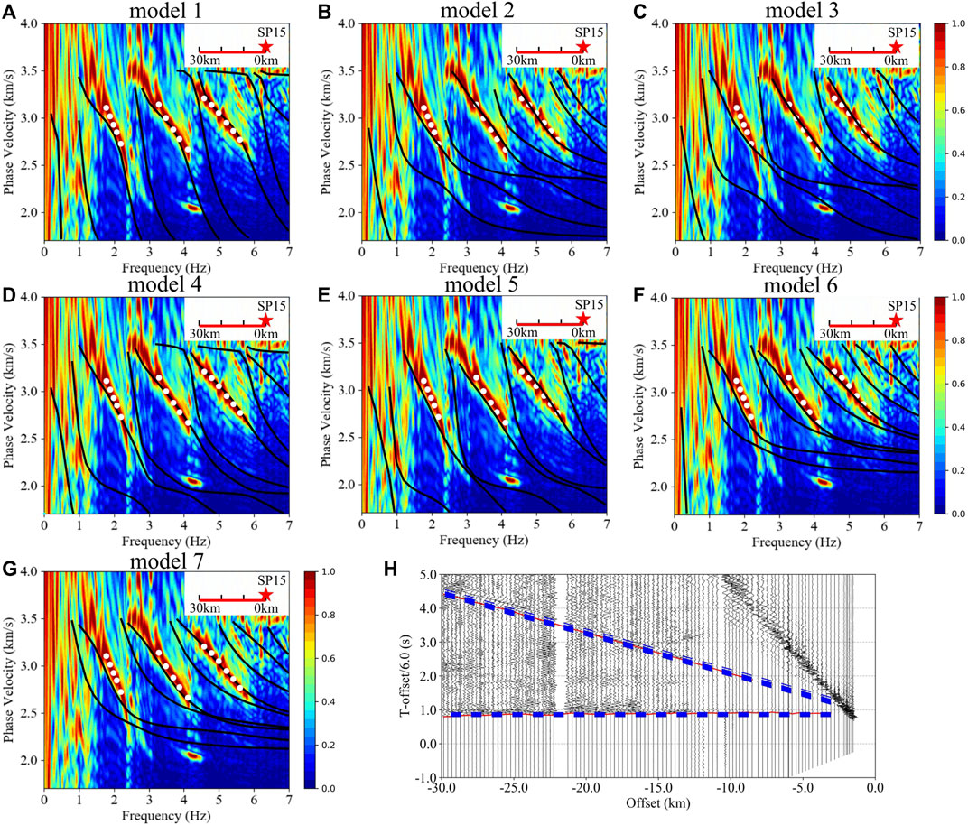
FIGURE 7. The results of the joint Monte Carlo inversion with the multimodal dispersion curves and the Pg and Sg travel times from the SP15 seismic data. In the upper right corner of (A–G), the red star represents the source, and the F-J spectrogram is extracted from the seismic data on the red line. (A–G) are the dispersion curves of the accepted models one to seven in Table 2. (H) The red lines are the picked Pg and Sg, and the blue dashed lines are the calculated Pg and Sg of the accepted models in Table 2.

TABLE 2

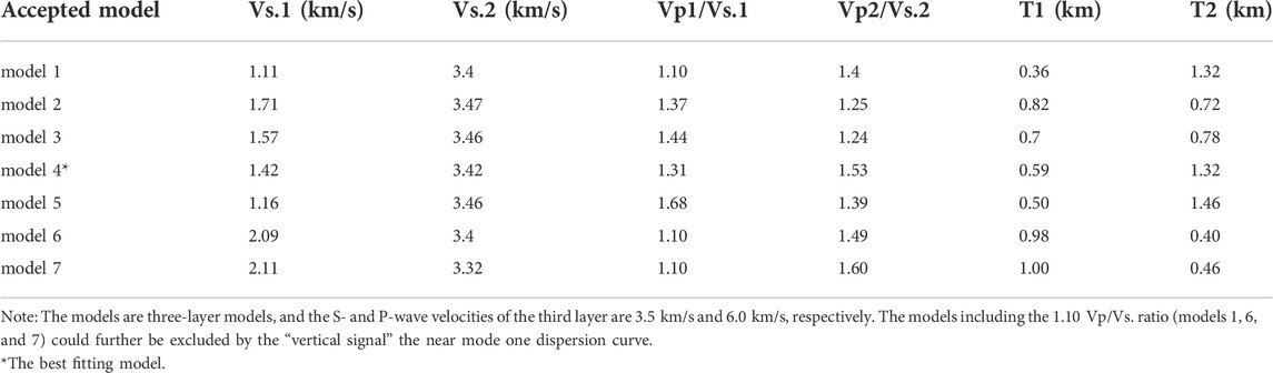
TABLE 2. The models fitting the SP15 seismic data.

FIGURE 8

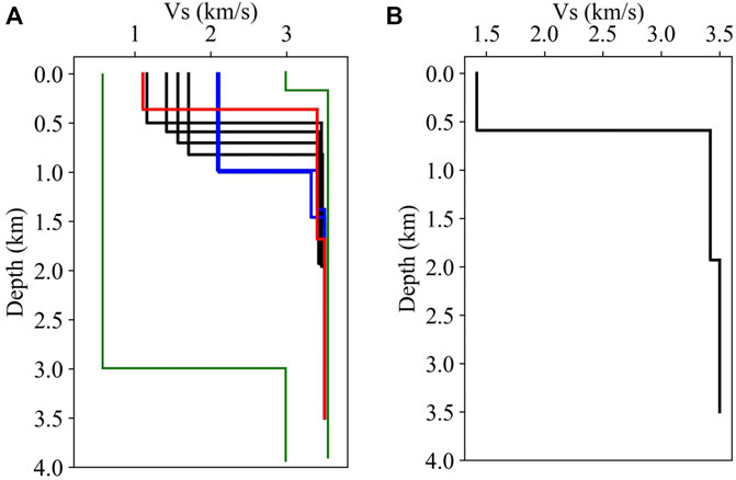
FIGURE 8. The accepted models in Table 2. (A) The green lines are the limits of the model parameters, and 10⁶ initial three-layer models were generated between the green lines. The red line represents model one in Table 2, the blue lines represent models six and seven in Table 2, and the black lines represent the other models. (B) The best fitting model (model four in Table 2).

In the analysis of the SP15 F-J spectrograms, it was not clear that the “vertical signal” near the mode one dispersion curve is a dispersion curve. The dispersion curves of accepted models two to five show that there is a dispersion curve near the “vertical signal”, suggesting that this “vertical signal” is the low-resolution image of a dispersion curve. By confirming that the “vertical signal” is a dispersion curve, it is further proved that the F-J method is an effective surface wave analysis method for DSS data. In addition, the models 1, 6, and seven could be excluded from the accepted models because: these models produce dispersion curves between the picked mode one and mode two dispersion curves, but these dispersion curves are far from the “vertical signal”.

3.2.3 The velocity models/2D velocity model constrained by the 10-km-long seismic record sections from SP15

The Rayleigh wave phase velocities shown in the 10 km-long F-J spectrograms of SP15 (Figures 5D–F) decrease gradually from west to the east (from 30 km offset to 0 km offset), while the sediment thickness presented by the drill hole data (Lawrence & Hoffman, 1993b) increases gradually from west to east. It seems that the variation in the Rayleigh wave phase velocities is caused by the variation of the sediment thickness (Socco & Boiero, 2008). Therefore, we changed the layer thicknesses of the best fitting model (model four in Table 2) to fit the F-J spectrograms extracted from the 10-km-long seismic record sections. We successively reduced the first layer thickness of mode four by 0.03 km, increased the first layer thickness of mode four by 0.02 km, and increased the first layer thickness of mode four by 0.08 km. Then the dispersion curves calculated from the corresponding 1D models could fit the spectrograms from the 20–30 km offset, 10–20 km offset and 0–10 km offset, respectively (Figure 9). The 2D shallow structure (Figure 9D) was then constructed by the three 1D models.

FIGURE 9

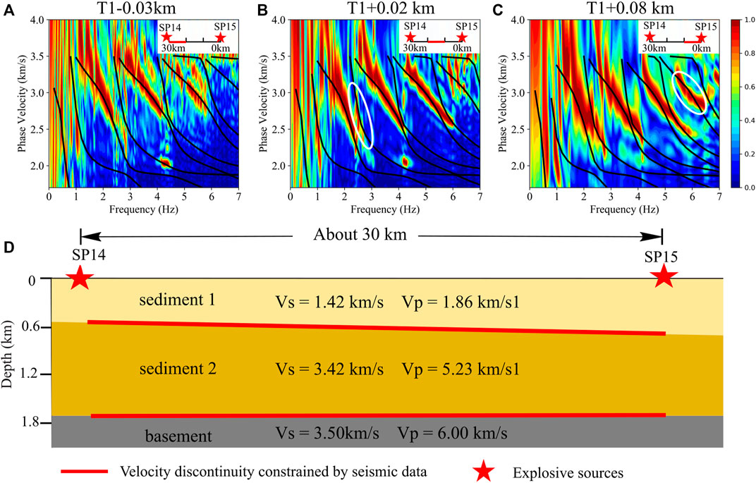
FIGURE 9. The analysis of the F-J spectrograms extracted from the 10-km-long seismic record sections. In the upper right corners of (A–C), the red stars represent the source, and the F-J spectrograms are extracted from the seismic data on the red lines. In the titles of (A–C), T1 represents the first layer thickness of the best fitting model (model 4) in Table 2. The F-J spectrograms in (A), (B), (C) are extracted from the 20–30 km offset, 10–20 km offset, and 0–10 km offset of SP15 seismic data respectively. The dispersion curves in each F-J spectrogram were calculated by (A) the model obtained by subtracting 0.03 km from the first layer thickness of model 4; (B) the model obtained by adding 0.02 km to the first layer thickness of model four; and (C) the model obtained by adding 0.08 km to the first layer thickness of model 4. (D) The 2D minimum-structure model constructed by combining the three 1D models of (A–C).

4 Discussion

4.1 The sensitivity of the seismic data

To explore the sensitivity of the multimodal dispersion curves and the Pg and Sg traveltimes, we performed Monte Carlo inversion with the subset data of the SP11 and SP15 data.

4.1.1 The sensitivity of the SP11 seismic data

In the Piedmont, the reduced Pg traveltimes (Figure 2A) are slightly larger than zero, suggesting that a thin layer should exist on the surface. However, detailed information about this layer cannot be constrained by the Pg and Sg traveltimes inversion (Guo et al., 2019), indicating that the Pg and Sg traveltimes are not sensitive to the velocity and thickness of this layer.

We performed the Monte Carlo inversion only with the fundamental dispersion curve (the picked mode 1), and the low-resolution layered structure on the surface (black lines in Figure 10) was constrained by the fundamental dispersion curve. With the joint inversion of the fundamental dispersion curve and the Pg and Sg traveltimes, the bottom layer velocity could be further constrained (blue lines in Figure 10), demonstrating that the Pg and Sg traveltimes are mainly sensitive to the velocity of the bottom layer. With the joint inversion of the fundamental and first dispersion curves, both the velocities and thickness were further constrained, and the range of the accepted models (red lines in Figure 10) is close to the range of the models accepted by the joint inversion of the multimodal dispersion curves and the Pg and Sg traveltimes (Figure 6). It is suggested that the multimodal dispersion curves could be sensitive to both the velocity and layer thickness and that the body wave traveltimes only play a minor role in the joint inversion of SP11 data.

FIGURE 10

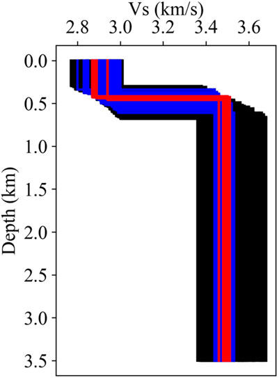
FIGURE 10. The inversion results with the subset data of the SP11 seismic data. The black lines are models obtained by the fundamental dispersion curve; blue lines are models obtained by the joint inversion of the fundamental dispersion curve and the Pg and Sg traveltimes; and red lines are models obtained by the joint inversion of the fundamental and first dispersion curves.

4.1.2 The sensitivity of the SP15 seismic data

In the ACP, the Pg reduced times are nearly flat between the 0 km offset and 30 km offset of SP15 (Figure 2B), while there are obvious differences between the 10-km-long F-J spectrograms (Figures 5D–F), suggesting that the dispersion curves are more sensitive to lateral variation in the sediment structure than the refraction traveltimes. The variation in the first layer thickness of the 2D model does not introduce significant errors in the Pg and Sg traveltimes, confirming that the multimodal dispersion curves could be much more sensitive to the first sedimentary layer thickness than the refraction traveltimes.

We adjusted the second layer thickness of the accepted models and found that halving the thickness of the second layer did not introduce significant errors into the dispersion curves, suggesting that the dispersion curves exerted little constraint on the second layer. Because the Pg and Sg traveltimes are determined by the basement velocity and the quotient of sedimentary thickness and velocity, the Pg and Sg traveltimes also provide little constraint on the second layer.

Although both the dispersion curves and the body wave traveltimes exerted little constraint on the second layer, this layer was still constrained by the joint inversion of the dispersion curves and the Pg and Sg traveltimes, suggesting that the join inversion of body waves and surface waves is an effective way to improve the resolution of subsurface structures. We performed the joint inversions with the multimodal dispersion curves and Sg traveltimes, and the results were presented in Figures 11A,B. We also performed the joint inversions with the multimodal dispersion curves and Pg traveltimes respectively, and the results were presented in Figures 11C,D. The contradictory results accepted by different subset data (Figures 11A,B and Figures 11C,D) demonstrate that a completed seismic dataset, including the surface waves and the P-and S- body waves, is helpful to constrain the fine subsurface structure.

FIGURE 11

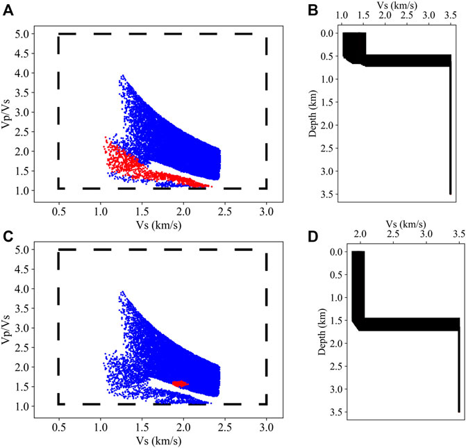
FIGURE 11. The inversion results with the subset data of the SP15 seismic data. A total of 10⁶ two-layer models were randomly generated in the model space outlined by the black dashed box in (A) and (C). The blue dots in (A) and (C) are the models accepted by multimodal dispersion curves. The red dots in (A) are the models accepted by the multimodal dispersion curves and the Sg traveltimes, and the red dots in (C) are the models accepted by the multimodal dispersion curves and Pg traveltimes. (B) and (D) present accepted models (the red dots in (a) and (C)) with the Vs-depth relation. The contradictory results accepted by different subset data demonstrate that it is important to use both the surface waves and the P-and S-body waves to constrain the subsurface structure.

4.2 Comparisons with the existing results

In the Piedmont, the velocities of the thin layer agree with the near-surface velocities constrained by the seismic-wave propagation of the Mw5.8 earthquake (Figure 12, Pollitz and Mooney, 2014). In the ACP, our study revealed a two-layer sediment structure, while only one sediment layer was identified by conventional DSS data processing (Guo et al., 2019). The offshore ENAM-CSE seismic lines (Figure 12) indicate that the sediment in the ocean consists of two layers (Shuck et al., 2019; Lynner et al., 2020), and the P-wave velocities in the ocean sedimentary layers are approximately consistent with the P-wave velocities in our models. Catchings et al. (2008) (Figure 12) constrained the shallow P-wave velocity structure of the ACP with a 30 km-long shallow seismic reflection/refraction survey in Delmarva Peninsula, Virginia, and the P-wave tomograph they presented is also approximately consistent with the two-layer sediment structure obtained by our study. With the results from Shuck et al. (2019), Catchings et al. (2008) and our study, we infer that the two-layer sediment structure extends from the ocean to the land.

FIGURE 12

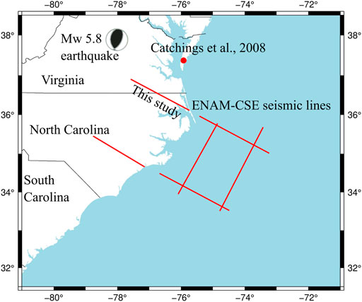
FIGURE 12. The locations of the existing studies near our study area. The red lines are the onshore and offshore seismic lines constructed by the ENAM-CSE. Red dot represents the location discussed in Catchings et al. (2008), and the focal sphere is the Mw 5.8 earthquake in Virginia.

The sedimentary Vp/Vs. ratios constrained by this study are much lower than the empirical values (Brocher, 2005), but experimental data samples have shown that extremely low sedimentary Vp/Vs. ratios are not unusual (Kassab & Weller, 2015; Zaitsev et al., 2017). Combined with the surface lithology (King& Beikman 1974; Glover & Klitgord 1995) in the ACP and the studies on low sedimentary Vp/Vs. ratios (Gregory, 1976; Christensen, 1996; Salem, 2000; Brocher, 2005; Mavko et al., 2009; Kassab & Weller, 2015), we inferred that the low Vp/Vs. ratios in this study may be associated with high quartz content (Christensen, 1996; Brocher, 2005) and/or groundwater undersaturation (Gregory, 1976; Christensen, 1996; Salem, 2000; Mavko et al., 2009; Kassab & Weller, 2015; Berg et al., 2021).

5 Conclusion

In this study, we extracted the multimodal dispersion curves from DSS data in the Piedmont and ACP with the F-J method and constrained the shallow velocity structure with the Monte Carlo inversion of the multimodal dispersion curves and the body wave refraction traveltimes. A ∼0.42 km thick layer in the Piedmont and a two-layer sediment structure in the ACP are effectively constrained by the joint inversions. These subsurface structures are not identified in the conventional DSS data processing, indicating that the resolution of the shallow/near-surface structure (0–2 km depth) could be improved by extracting dispersion curves from the DSS data.

Since clear surface waves are also observed and consider noise in deep seismic reflection and shallow seismic reflection/refraction experiments, it is suggested that analysis of surface waves recorded by these seismic experiments would also be worthwhile.

Data availability statement

Publicly available datasets were analyzed in this study. This data can be found here: The data are stored in International Federation of Digital Seismograph Networks (Magnani et al., 2015, doi: 10.7914/SN/ZI_2015), Interdisciplinary Earth Data Alliance (IEDA) (Magnani et al., 2018, doi: 10.1594/ IEDA/500088).

Author contributions

All of the authors contributed to this manuscript. WG and ZL analyzed the surface waves and wrote the manuscript draft; WG and SZ analyzed the body waves and collected the references; and WG contributed to the inversion. XC and ZL contributed to the conception and design of the study.

Funding

This work was supported by the National Natural Science Foundation of China (Grants No. 41790465, U1901602, 42074070, and 42104048), Shenzhen Key Laboratory of Deep Offshore Oil and Gas Exploration Technology (Grant No. ZDSYS20190902093007855), the National Key R and D Program of China (2017YFC1500204), the China Postdoctoral Science Foundation (Grant No. 2021M691406), and the China Earthquake Science Experiment Project (202107086728).

Acknowledgments

The collection of these data was coordinated by Southern Methodist University and the Woods Hole Oceanographic Institution. We are grateful to the dedicated twenty-person field crew from various universities, the USGS and two IRIS-PASSCAL technicians who participated in the field. Seismic sources were coordinated by S. Harder and others from UT-El Paso. We gratefully acknowledge the ENAM-CSE principal investigators: Harm van Avendonk, Donna Shillington, Beatrice Magnani, Dan Lizarralde, Brandon Dugan, Matt Hornback, Steven Harder, Anne Bécel, Jim Gaherty, Maureen Long, Gail Christeson, Lara Wagner, and Maggie Benoit. The Python package containing the F-J method (CC-FJpy, Li et al., 2021) can be obtained from http://dx.doi.org/10.1785/0220210042. A slim Python wrapper around the program ‘surf96’ from “Computer programs in seismology” by R. Herrmann (2013) (http://www.eas.slu.edu/eqc/eqccps.html) was used to calculate the layer model dispersion curves in this study (https://github.com/miili/pysurf96).

Conflict of interest

The authors declare that the research was conducted in the absence of any commercial or financial relationships that could be construed as a potential conflict of interest.

Publisher’s note

All claims expressed in this article are solely those of the authors and do not necessarily represent those of their affiliated organizations, or those of the publisher, the editors and the reviewers. Any product that may be evaluated in this article, or claim that may be made by its manufacturer, is not guaranteed or endorsed by the publisher.

Supplementary material

The Supplementary Material for this article can be found online at: https://www.frontiersin.org/articles/10.3389/feart.2022.1025935/full#supplementary-material

References

Anggono, T., SyuhadaFebriani, F., Soedjatmiko, B., and Amran, A. (2018). Investigation of sediment thickness effect to the receiver function through forward modelling. J. Phys. Conf. Ser. 985, 012014. doi:10.1088/1742-6596/985/1/012014

CrossRef Full Text | Google Scholar

Benz, H. M., Unger, J. D., Leith, W. S., Mooney, W. D., Solodilov, L., Egorkin, A. V., et al. (1992). Deep-seismic sounding in northern Eurasia. Eos Trans. AGU. 73 (28), 297. doi:10.1029/91EO00233

CrossRef Full Text | Google Scholar

Berg, E. M., Lin, F., Schulte-Pelkum, V., Allam, A., Qiu, H., and Gkogkas, K. (2021). Shallow crustal shear velocity and vp/vs across southern California: Joint inversion of short-period Rayleigh wave ellipticity, phase velocity, and teleseismic receiver functions. Geophys. Res. Lett. 48 (15). doi:10.1029/2021GL092626

CrossRef Full Text | Google Scholar

Bevington, P. R. (1969). Data reduction and error analysis for the physical sciences. New York: McGraw-Hill.

Google Scholar

Braile, L. W., and Smith, R. B. (1975). Guide to the interpretation of crustal refraction profiles. Geophys. J. Int. 40 (2), 145–176. doi:10.1111/j.1365-246X.1975.tb07044.x

CrossRef Full Text | Google Scholar

Brocher, T. M. (2005). Empirical relations between elastic wavespeeds and density in the earth’s crust. Bull. Seismol. Soc. Am. 95 (6), 2081–2092. doi:10.1785/0120050077

CrossRef Full Text | Google Scholar

Catchings, R. D., Powars, D. S., Gohn, G. S., Horton, J. W., Goldman, M. R., and Hole, J. A. (2008). Anatomy of the chesapeake bay impact structure revealed by seismic imaging, Delmarva Peninsula, Virginia, USA: Chesapeake bay impact structure. J. Geophys. Res. 113 (B8). doi:10.1029/2007JB005421

CrossRef Full Text | Google Scholar

Christensen, N. I. (1996). Poisson’s ratio and crustal seismology. J. Geophys. Res. 101 (B2), 3139–3156. doi:10.1029/95JB03446

CrossRef Full Text | Google Scholar

Constable, S. C., Parker, R. L., and Constable, C. G. (1987). Occam’s inversion: A practical algorithm for generating smooth models from electromagnetic sounding data. Geophysics 52, 289–300. doi:10.1190/1.1442303

CrossRef Full Text | Google Scholar

Cunningham, E., and Lekic, V. (2020). Constraining properties of sedimentary strata using receiver functions: An example from the atlantic Coastal Plain of the southeastern United States. Bull. Seismol. Soc. Am. 110 (2), 519–533. doi:10.1785/0120190191

CrossRef Full Text | Google Scholar

Duan, Y., Wang, F., Zhang, Lin J., Liu, Z., Liu, B., Yang, Z., et al. (2016). Three-dimensional crustal velocity structure model of the middle-eastern north China Craton (HBCrust1.0). Sci. China Earth Sci. 59, 1477–1488. doi:10.1007/s11430-016-5301-0

CrossRef Full Text | Google Scholar

Essien, U. E., Akankpo, A. O., and Igboekwe, M. U. (2014). Poisson’s ratio of surface soils and shallow sediments determined from seismic compressional and shear wave velocities. Int. J. Geosciences 05 (12), 1540–1546. doi:10.4236/ijg.2014.512125

CrossRef Full Text | Google Scholar

Fischer, K. M., Salvati, L. A., HoughGonzalezNelsen, S. E. E. C. E., and Roth, E. G. (1995). Sediment-induced amplification in the northeastern United States: A case study in providence, Rhode Island. Bull. Seismol. Soc. Am. 85 (5), 1388–1397. doi:10.1785/bssa0850051388

CrossRef Full Text | Google Scholar

Frankel, A. (2009). A constant stress-drop model for producing broadband synthetic seismograms: Comparison with the next generation attenuation relations. Bull. Seismol. Soc. Am. 99, 664–680. doi:10.1785/0120080079

CrossRef Full Text | Google Scholar

Giese, P., Prodehl, C., and Stein, A. (1976). Explosion seismology in central europe: Data and results. Berlin/Heidelberg, Germany: Springer-Verlag.

Google Scholar

Glover, L., and Klitgord, K. D. (1995). E-3 southwestern Pennsylvania to baltimore canyon trough. Boulder, United States: Geological Society of America. doi:10.1130/DNAG-COT-E-3

CrossRef Full Text | Google Scholar

Gregory, A. R. (1976). Fluid saturation effects on dynamic elastic properties of sedimentary rocks. Geophysics 41, 895–921. doi:10.1190/1.1440671

CrossRef Full Text | Google Scholar

Guo, W., Zhao, S., Wang, F., Yang, Z., Jia, S., and Liu, Z. (2019). Crustal structure of the eastern Piedmont and Atlantic coastal plain in North Carolina and Virginia, eastern North American margin. Earth Planets Space 71 (1), 69. doi:10.1186/s40623-019-1049-z

CrossRef Full Text | Google Scholar

Herrmann, R. B. (2013). Computer programs in seismology: An evolving tool for instruction and research. Seismol. Res. Lett. 84, 1081–1088. doi:10.1785/0220110096

CrossRef Full Text | Google Scholar

Hübscher, C., and Gohl, K. (2014). “Reflection/refraction seismology,” in Encyclopedia of marine geosciences. Editors J. Harff, M. Meschede, S. Petersen, and J. Thiede Dordrecht: Springer Netherlands, 1–15. doi:10.1007/978-94-007-6644-0_128-1

CrossRef Full Text | Google Scholar

Kassab, M. A., and Weller, A. (2015). Study on P-wave and S-wave velocity in dry and wet sandstones of Tushka region, Egypt. Egypt. J. Petroleum 24 (1), 1–11. doi:10.1016/j.ejpe.2015.02.001

CrossRef Full Text | Google Scholar

Keskar, N. R., and Chelikowsky, J. R. (1992). Negative Poisson ratios in crystalline SiO₂ from first-principles calculations. Nature 358, 222–224. doi:10.1038/358222a0

CrossRef Full Text | Google Scholar

King, P. B., and Beikman, H. M. (1974). Geologic map of the United States: U.S. Geol. Surv. scale 1 (2), 500, 000.

Google Scholar

Kosminskaya, I. P. (1971). “Deep seismic sounding and its relation to other seismic methods,” in Deep seismic sounding of the earth’s crust and upper mantle (Boston, MA: Springer). doi:10.1007/978-1-4684-7867-9_1

CrossRef Full Text | Google Scholar

Lawrence, D. P., and Hoffman, C. W. (1993b). Geology of basement rocks beneath the North Carolina Coastal Plain. N.C. Geol. Surv, North Carolina.

Google Scholar

Lawrence, D. P., and Hoffman, C. W. (1993a). Interpretive geologic map of basement rocks beneath the North Carolina Coastal Plain. N. C. Geol. Surv. Bull. 95, 60. 1 plate.

Google Scholar

Li, J., Song, X., Zhu, L., and Deng, Y. (2017). Joint inversion of surface wave dispersions and receiver functions with P velocity constraints: Application to southeastern tibet: Joint inversion and application to tibet. J. Geophys. Res. Solid Earth 122 (9), 7291–7310. doi:10.1002/2017JB014135

CrossRef Full Text | Google Scholar

Li, J., Tang, Y., Wu, T., Zhao, J., Wu, H., Wu, W., et al. (2020). Overpressure origin and its effects on petroleum accumulation in the conglomerate oil province in Mahu Sag, Junggar Basin, NW China. Petroleum Explor. Dev. 47 (4), 726–739. doi:10.1016/S1876-3804(20)60088-X

CrossRef Full Text | Google Scholar

Li, S., Mooney, W. D., and Fan, J. (2006). Crustal structure of mainland China from deep seismic sounding data. Tectonophysics 420 (1–2), 239–252. doi:10.1016/j.tecto.2006.01.026

CrossRef Full Text | Google Scholar

Li, X., Chen, X., Yang, Z., Wang, B., Yang, B., Tao, G., et al. (2020). Application of high-order surface waves in shallow exploration: An example of the Suzhou river, Shanghai. Chin. J. Geophys. (in Chinese) 63 (1), 247–263.e1. doi:10.1016/j.ajodo.2019.08.014

CrossRef Full Text | Google Scholar

Li, Z., and Chen, X. (2020). An effective method to extract overtones of surface wave from array seismic records of earthquake events. J. Geophys. Res. Solid Earth 125. doi:10.1029/2019JB018511

CrossRef Full Text | Google Scholar

Li, Z., Shi, C., and Chen, X. (2021a). Constraints on crustal P-wave structure with leaking mode dispersion curves. Geophysical Research Letters 48, e2020GL091782. doi:10.1029/2020GL091782

CrossRef Full Text | Google Scholar

Li, Z., Zhou, J., Wu, G., Wang, J., Zhang, G., Dong, S., et al. (2021b). CC-FJpy: A Python package for extracting overtone surface-wave dispersion from seismic ambient-noise cross correlation. Seismological Research Letters XX, 3179–3186.

CrossRef Full Text | Google Scholar

Lin, J., Mooney, W. D., Wang, F., Duan, Y., Tian, X., Xu, T., et al. (2019). Crustal P wave velocity structure beneath the SE margin of the Tibetan Plateau from Deep Seismic Sounding results. Tectonophysics 755, 109–126. doi:10.1016/j.tecto.2019.01.010

CrossRef Full Text | Google Scholar

Lu, L., and Zhang, B. (2006). Inversion of Rayleigh waves using a genetic algorithm in the presence of a low-velocity layer. Acoust. Phys. 52, 701–712. doi:10.1134/S106377100606011X

CrossRef Full Text | Google Scholar

Lynner, C., Van Avendonk, J. A. H., Bécel, A., Christeson, G. L., Dugan, B., Gaherty, J. B., et al. (2020). The Eastern North American margin community seismic experiment: An amphibious active and passive-source dataset. Seismological Research Letters 91 (1), 533–540. doi:10.1785/0220190142

CrossRef Full Text | Google Scholar

Magnani, M. B., Harder, S., and Lizarralde, (2018). Explosion seismic refraction data acquired on land in eastern North Carolina and virgina as part of the Eastern North American Margin (ENAM) community seismic experiment (CSE) (2015). New York, Palisades: Interdisciplinary Earth Data Alliance IEDA.

Google Scholar

Magnani, M. B., Lizarralde, D., and Harder, S. (2015). “A community seismic experiment targeting the pre-syn, post-rift evolution of the Mid-Atlantic US: The ENAM CSE land active source experiment,” in International federation of digital seismograph Networks, Dataset/Seismic Network.431-438 doi:10.7914/SN/ZI_2015

CrossRef Full Text | Google Scholar

Maraschini, M., Ernst, F., Foti, S., and Socco, L. V. (2010). A new misfit function for multimodal inversion of surface waves. Geophysics 75 (4), G31–G43. doi:10.1190/1.3436539

CrossRef Full Text | Google Scholar

Maraschini, M., and Foti, S. (2010). A Monte Carlo multimodal inversion of surface waves: Monte Carlo multimodal surface wave inversion. Geophys. J. Int. 182 (3), 1557–1566. doi:10.1111/j.1365-246X.2010.04703.x

CrossRef Full Text | Google Scholar

Marzen, R. E., Shillington, D. J., Lizarralde, D., and Harder, S. H. (2019). Constraints on appalachian orogenesis and continental rifting in the southeastern United States from wide-angle seismic data. J. Geophys. Res. Solid Earth 124 (7), 6625–6652. doi:10.1029/2019JB017611

CrossRef Full Text | Google Scholar

Marzen, R. E., Shillington, D. J., Lizarralde, D., Knapp, J. H., Heffner, D. M., Davis, J. K., et al. (2020). Limited and localized magmatism in the central atlantic magmatic province. Nat. Commun. 11 (1), 3397. doi:10.1038/s41467-020-17193-6

PubMed Abstract | CrossRef Full Text | Google Scholar

Mavko, G., Mukerji, T., and Dvorkin, J. (2009). “The rock physics handbook,” in Tools for seismic analysis in porous media. second edition (Cambridge, U.K: Cambridge University Press).

Google Scholar

Mooney, W. D., Laske, G., and Masters, T. G. (1998). Crust 5.1: A global crustal model at 5° × 5°. J. Geophys. Res., 103, 727–747. doi:10.1029/97JB02122

CrossRef Full Text | Google Scholar

Musacchio, G., Mooney, W. D., Luetgert, J. H., and Christensen, N. I. (1997). Composition of the crust in the grenville and appalachian provinces of north America inferred from V_P/V_Sratios. J. Geophys. Res. 102 (B7), 15225–15241. doi:10.1029/96JB03737

CrossRef Full Text | Google Scholar

Pakiser, L. C., and Mooney, W. D. (1989). Geophysical framework of the continental United States, Vol. 172. Boulder: Geological Society of America Memoir.

Google Scholar

Park, C. B., Miller, R. D., Xia, J., and Ivanov, J. (2007). Multichannel analysis of surface waves (MASW)—Active and passive methods. The Leading Edge 26 (1), 60–64. doi:10.1190/1.2431832

CrossRef Full Text | Google Scholar

Pollitz, F. F., and Mooney, W. D. (2014). Regional seismic-wave propagation from the M5. 8 23 August 2011, Mineral, Virginia, earthquake. Geological Society of America Special Papers 509. , SPE509–06.

Google Scholar

Pratt, T. L. (2018). Characterizing and imaging sedimentary strata using depth-converted spectral ratios: An example from the atlantic Coastal Plain of the eastern United States. Bull. Seismol. Soc. Am. 108 (5A), 2801–2815. doi:10.1785/0120180046

CrossRef Full Text | Google Scholar

Salem, H. S. (2000). Poisson’s ratio and the porosity of surface soils and shallow sediments, determined from seismic compressional and shear wave velocities. Géotechnique 50 (4), 461–463. doi:10.1680/geot.2000.50.4.461

CrossRef Full Text | Google Scholar

Schleicher, L. S., and Pratt, T. L. (2021). Characterizing fundamental resonance peaks on flat-lying sediments using multiple spectral ratio methods: An example from the atlantic Coastal Plain, eastern United States. Bull. Seismol. Soc. Am. 111 (4), 1824–1848. doi:10.1785/0120210017

CrossRef Full Text | Google Scholar

Shuck, B. D., Van Avendonk, H. J. A., and Bécel, A. (2019). The role of mantle melts in the transition from rifting to seafloor spreading offshore eastern North America. Earth and Planetary Science Letters 525, 115756. doi:10.1016/j.epsl.2019.115756

CrossRef Full Text | Google Scholar

Socco, L. V., and Boiero, D. (2008). Improved Monte Carlo inversion of surface wave data. Geophys. Prospect. 56 (3), 357–371. doi:10.1111/j.1365-2478.2007.00678.x

CrossRef Full Text | Google Scholar

Socco, L. V., and Strobbia, C. (2004). Surface-wave method for near-surface characterization: A tutorial. Near Surface Geophysics 2 (4), 165–185. doi:10.3997/1873-0604.2004015

CrossRef Full Text | Google Scholar

Sun, N., Pan, L., Wang, W., Ye, B., Wang, B., and Chen, X. (2021). Inversion of shear wave velocity structure beneath the Binchuan airgun source area using a nested combination of multi-scale arrays. Chinese Journal of Geophysics 64 (11), 4012–4021. doi:10.6038/cjg2021P0064

CrossRef Full Text | Google Scholar

Wang, J., Wu, G., and Chen, X. (2019). Frequency-bessel transform method for effective imaging of higher-mode Rayleigh dispersion curves from ambient seismic noise data. J. Geophys. Res. Solid Earth 124 (4), 3708–3723. doi:10.1029/2018JB016595

CrossRef Full Text | Google Scholar

Wu, G., Pan, L., Wang, J., and Chen, X. (2020). Shear velocity inversion using multimodal dispersion curves from ambient seismic noise data of USArray transportable array. J. Geophys. Res. Solid Earth 125 (1), e2019JB018213. doi:10.1029/2019jb018213

CrossRef Full Text | Google Scholar

Wu, H., Chen, X., and Pan, L. (2019). S-wave velocity imaging of the Kanto basin in Japan using the frequency-Bessel transformation method. Chinese J. Geophys. (in Chinese) 62 (9), 3400–3407. doi:10.6038/cjg2019N0205

CrossRef Full Text | Google Scholar

Xi, C., Xia, J., Mi, B., Dai, T., Liu, Y., and Ning, L. (2021). Modified frequency-bessel transform method for dispersion imaging of Rayleigh waves from ambient seismic noise. Geophysical Journal International 225 (2), 1271–1280. doi:10.1093/gji/ggab008

CrossRef Full Text | Google Scholar

Yang, Z., Chen, X ., Pan, L., Wang, J., Xu, J., and Zhang, D. (2019). Multi-channel analysis of Rayleigh waves based on the vector wavenumber tansformation method (VWTM). Chinese J. Geophys. (in Chinese) 62 (1), 298–305. doi:10.6038/cjg2019M0641

CrossRef Full Text | Google Scholar

Zaitsev, V. Y., Radostin, A. V., Pasternak, E., and Dyskin, A. (2017). Extracting real-crack properties from non-linear elastic behaviour of rocks: Abundance of cracks with dominating normal compliance and rocks with negative Poisson ratios. Nonlinear Process. Geophys. 24 (3), 543–551. doi:10.5194/npg-24-543-2017

CrossRef Full Text | Google Scholar

Zelt, C. A., and Barton, P. J. (1998). Three-dimensional seismic refraction tomography: A comparison of two methods applied to data from the faeroe basin. J. Geophys. Res. 103 (B4), 7187–7210. doi:10.1029/97JB03536

CrossRef Full Text | Google Scholar

Zelt, C. A., and Forsyth, D. A. (1994). Modeling wide-angle seismic data for crustal structure: Southeastern Grenville Province. J. Geophys. Res. 99 (B6), 11687–11704. doi:10.1029/93JB02764

CrossRef Full Text | Google Scholar

Zelt, C. A. (1999). Modelling strategies and model assessment for wide-angle seismic traveltime data. Geophysical Journal International 139 (1), 183–204. doi:10.1046/j.1365-246X.1999.00934.x

CrossRef Full Text | Google Scholar

Zelt, C. A., and Smith, R. B. (1992). Seismic traveltime inversion for 2-D crustal velocity structure. Geophysical Journal International 108 (1), 16–34. doi:10.1111/j.1365-246x.1992.tb00836.x

CrossRef Full Text | Google Scholar

Zhan, W., Pan, L., and Chen, X. (2020). A widespread mid-crustal low-velocity layer beneath Northeast China revealed by the multimodal inversion of Rayleigh waves from ambient seismic noise. Journal of Asian Earth Sciences 196, 104372. doi:10.1016/j.jseaes.2020.104372

CrossRef Full Text | Google Scholar

Zhao, S., and Guo, W. (2019). Crustal structure of eastern North Carolina: Piedmont and Coastal Plain. Bull. Seismol. Soc. Am. 109 (6), 2288–2304. doi:10.1785/0120180281

CrossRef Full Text | Google Scholar

Zhou, J., and Chen, X. (2021). Removal of crossed artifacts from multimodal dispersion curves with modified frequency–bessel method. Bull. Seismol. Soc. Am. 112 (1), 143–152. doi:10.1785/0120210012

CrossRef Full Text | Google Scholar