Sensitivity analysis of anisotropic parameter inversion simultaneously with microseismic source location in layered VTI media

The hypocenters of microseismic events induced by hydraulic fracturing are conventionally located with an initial model established from well logs or perforation shots. In most geological settings, the arrival times are insufficiently explained without accounting for the velocity changes introduced by the reservoir stimulation process. The model parameters and source locations should be inverted simultaneously with arrival time information. Therefore, the joint inversion of event locations and velocity model requires the information of anisotropy parameters, which leads to the problem of the selection of degree of symmetry of anisotropic media in the inversion process. Since it is not possible to retrieve all elastic moduli from limited passive seismic data, the joint inversion is constrained to layered vertical transversely isotropic (VTI) media. Various methods have been proposed to invert the velocity model and source locations from the arrival times in anisotropic media, but the number of retrievable parameters in different parametrization types and acquisition scenarios have not been decisively discussed. We analyze the sensitivities for event locations and anisotropic parameters by the singular value decomposition (SVD) of the Fréchet derivatives in a layered anisotropic medium with vertical axis of symmetry. The singular values and eigenvectors obtained from SVD can be used to predict which unknown parameters are better constrained by the available traveltimes. The comparison of different parametrizations and monitoring array configurations allows to design a better inversion strategy to provide microseismic event locations and anisotropic parameters.

1 Introduction

Microseismic monitoring is an important diagnostic tool for hydraulic fracturing stimulation in unconventional reservoirs (Grechka, 2010; Maxwell et al., 2010; Li et al., 2019b; Pan et al., 2022). Locating induced microseismic events is the primary task in such monitoring, which requires the accurate velocity model (Eisner et al., 2009; Zimmer et al., 2009; Li et al., 2020). Traditionally, the velocity models are derived from sonic logs and perforation shots (Pei et al., 2009; Bardainne and Gaucher, 2010). As the perforation shots illuminate limited subsurface, the locations are prone to errors due to the unreliable velocity information (Grechka et al., 2011; Li et al., 2013; Li et al., 2019a). Additionally, the hydraulic stimulation and fractured shales in the reservoir may change the velocity model. The estimated velocity models may be updated based on the information supplied by the microseismic events, which is similar to the passive seismic tomography in global seismology (Thurber, 1986; Zhang and Thureber, 2003).

As the anisotropy commonly exists in shale (Eisner et al., 2011; Tsvankin, 2012) and shear wave splitting is commonly observed (Grechka and Yaskevich, 2014; Grechka, 2015), the isotropic velocity models are most likely insufficient to explain the recorded traveltimes in the estimation of velocity simultaneously with event locations. For example, Grechka et al. (2011) show that event locations lead to lower residuals when anisotropy is taken into account. Grechka and Duchkov (2011) propose that isotropic model is inadequate and develop methodology to estimate elements of elastic moduli from traveltimes observed in downhole geophones. The challenge of the inversion is that the phase and group velocities are represented in narrow angular apertures for typical downhole geometries. Grechka et al. (2011) estimated the anisotropy simultaneously with events locations in a single-well geometry. The analysis is based on stiffness tensor and only the downhole case is discussed. Li et al. (2013) proposed to use differential arrival times and differential azimuths for event location and anisotropic tomography, which is also discussed in a single well geometry. Grechka and Yaskevich (2014) used the traveltimes and polarizations to invert event locations and parameters for layer triclinic media using downhole microseismic data with wide aperture. Michel and Tsvankin (2016) developed an elastic waveform inversion algorithm to estimate the anisotropic parameter and source information in the layered vertical transversely isotropic (VTI) media. In this study, we do not use full waveforms as the amplitude is often contaminated by noise and compromised by receiver coupling in downhole monitoring. The arrival times of the direct P- and S- waves sometimes are more reliable than the waveforms in the source location.

In the above discussed studies, the downhole geophones in a single vertical monitoring well are usually assumed and the elastic stiffness tensor is used to delineate the anisotropic properties. Alternatively, surface or near-surface arrays are also used in monitoring hydraulic fracturing (Duncan and Eisner, 2010). In such geometry most of the rays travel through overburden which can be characterized as vertical transversely isotropic media (VTI), and it is enough to describe the observed direct arrival times in field data (Gei et al., 2011).

In this study, we derive the analytical sensitivities for the elastic moduli and Thomsen-type parameters (Thomsen, 1986) in the joint inversion of event locations, source origin times and anisotropic properties with layered anisotropy assumption. We investigate the sensitivities of the direct P- and S- arrival time inversion to source location and anisotropic parameters by using singular value decomposition (SVD). We compare the sensitivity matrices derived from microseismic data for downhole geometry and establish the methodology to judge the effectiveness and limits of using the traveltimes to invert the unknown parameters.

2 Methodology

2.1 Joint inversion of microseismic location and anisotropic parameters

The objective function in the joint inversion of the source location, origin times and anisotropic tomography is the traveltime differences between the observed arrival time and the corresponding modelled arrival time. The sensitivities of the arrival time with respect to the hypocenter ${\mathit{x}}_i$, the origin times ${\tau }_i$, the anisotropic parameters $\mathit{m}$ and the layer thickness $l_j$ are given by the Fréchet derivativest

$\mathcal{F}=\left[\frac{\partial t_Q}{\partial \mathit{m}},\frac{\partial t_Q}{\partial {\mathit{x}}_i},\frac{\partial t_Q}{\partial {\tau }_i},\frac{\partial t_Q}{\partial l_j}\right],(1)$

where $t_Q$ is the arrival time and Q is used to denote the wave types, which can be quasi-P (qP), quasi-SV (qSV) or SH waves in the anisotropic media (Grechka and Duchkov, 2011). $\frac{\partial t_Q}{\partial \mathit{m}}$ are the derivatives of arrival times with respect to anisotropic parameters. Different parametrizations have been suggested to represent the anisotropic properties in homogeneous VTI medium. The first one is the combinaton of five elastic modulus, $c_{11}$, $c_{33}$, $c_{55}$, $c_{66}$, and $c_{13}$. Alternatively, Thomsen-type parameters can be used to define a VTI medium. Then $\mathit{m}$ includes the vertical P- and S-wave velocities, $V_{P0}$ and $V_{S0}$, and the anisotropic coefficients, $\epsilon ,\gamma$ and $\delta$. The derivatives can be calculated by the chain rule

$\frac{\partial t_Q}{\partial \mathit{m}}=\frac{\partial t_Q}{\partial g_Q}\frac{\partial g_Q}{\partial \mathit{m}}=-\frac{t_Q}{g_Q}\frac{\partial g_Q}{\partial \mathit{m}},(2)$

where $g_Q$ represents group velocities. The derivation of these derivatives for qP, qSV and SH is given in Supplementary Appendix S1.

The second part on the right side of Eq. 1 is the derivatives of traveltime $t_Q$ with respect to source location coordinates $\mathit{x}=\left\{x_1,x_2,x_3\right\}$. The location can be expressed by the event azimuth $\alpha$, radial distance $r$ and depth difference $h$ in a cylindrical coordinate system with the origin at the receiver.

$\mathit{x}=\left\{x_1,x_2,x_3\right\}=\left\{rcos\alpha ,rsin\alpha ,h\right\}.(3)$

In our joint inversion approach, the event azimuth is assumed to be known as they are independently measured from particle polarization, from the work of Eisner et al., 2009. The sensitivity of arrival times with respect to hypocenter can be expressed as

$\frac{\partial t_Q}{\partial \mathit{x}}=\frac{\partial t_Q}{\partial \left\{r,h\right\}}=-\left\{p_r^Q,p_h^Q\right\},(4)$

where $p_r^Q$ and $p_h^Q$ are the radial and vertical slowness, which are associated with anisotropic parameters and propagation angle.

The third part on the right side of Eq. 1 is the derivatives of arrival time $t_Q$ with respect to the origin times ${\tau }_i$. In the inversion, microseismic events are independently evaluated and the arrival time is only relevant with its own origin time. If the number of microseismic events is $n$, $\frac{\partial t_Q}{\partial {\tau }_i}$ is the $n\times n$ identity matrix. It’s equal to $I_{ij}$ for the j-th event.

The last part is the sensitivity with respect to the layer thickness. This problem has been discussed by Li et al. (2013). The sensitivity expression is

$\frac{\partial t_Q}{\partial l_j}=p_r^Q\left(\mathit{tan}{\phi }_2-\mathit{tan}{\phi }_1\right)+\frac{1}{\mathit{cos}{\phi }_1{g}_1^Q}-\frac{1}{\mathit{cos}{\phi }_2{g}_2^Q},(5)$

To specify the case to calculate the derivatives in the equations, here we assume the ray travels downwards, the terms should be adjusted in upward cases. ${\phi }_1$ and ${\phi }_2$ are the group angles in the first and second layer, respectively. $g_1^Q$ and $g_2^Q$ represent the corresponding group velocities.

As the derivatives $\left\{\frac{\partial t_Q}{\partial \mathit{m}},\frac{\partial t_Q}{\partial {\mathit{x}}_i},\frac{\partial t_Q}{\partial {\tau }_i},\frac{\partial t_Q}{\partial l_j}\right\}$ have different unit dimensions, they should be scaled by factors to balance the contributions from different unknowns (Grechka et al., 2011). Here the factors we choose are the mean source-receiver distance $f\left(x\right)=mean\left(\left|\mathit{x}\right|\right)$, the mean arrival times $f\left(\tau \right)=mean\left(\left|t_Q\right|\right)$ and the mean layer thickness $f\left(l\right)=mean\left(\left|l\right|\right)$. The matrix used in sensitivity analysis can be expressed as

$\mathcal{F}=\left[{\left(\frac{f\left(x\right)}{f\left(\tau \right)}\right)}^2\left\{\frac{\partial t_Q}{\partial c}\right\},f\left(x\right)\frac{\partial t_Q}{\partial {\mathit{x}}_i},f\left(\tau \right)\frac{\partial t_Q}{\partial {\tau }_i},f\left(l\right)\frac{\partial t_Q}{\partial l_j}\right],\mathrm{o}\mathrm{r}$

$\mathcal{F}=\left[\frac{f\left(x\right)}{f\left(\tau \right)}\left\{\frac{\partial t_Q}{\partial V_{P0}},\frac{\partial t_Q}{\partial V_{S0}}\right\},\left\{\frac{\partial t_Q}{\partial \epsilon ,},\frac{\partial t_Q}{\partial \gamma },\frac{\partial t_Q}{\delta }\right\},f\left(x\right)\frac{\partial t_Q}{\partial {\mathit{x}}_i},f\left(\tau \right)\frac{\partial t_Q}{\partial {\tau }_i},f\left(l\right)\frac{\partial t_Q}{\partial l_j}\right].(6)$

2.2 Singular value decomposition

Singular Value Decomposition (SVD) of a matrix is a factorization into three parts. It indicates the algebraic properties and provides important geometrical insights of the original matrix. The quantitative assessment of the joint inversion can be obtained by applying singular value decomposition to the Fréchet derivatives (Grechka et al., 2011; Kazei and Alkhalifah, 2018)

$\mathcal{F}=\mathit{u}\mathit{s}{\mathit{w}}^{\mathit{T}},(7)$

where $\mathit{u}$ is an orthogonal matrix and consists of eigenvectors of ${\mathcal{F}\mathcal{F}}^{\mathit{T}}$, $\mathit{s}$ is a diagonal matrix with singular values on the diagonal, $\mathit{w}$ is an orthogonal eigenvector matrix and consists of eigenvectors of ${\mathcal{F}}^{\mathit{T}}\mathcal{F}$, and ${\mathit{w}}^{\mathit{T}}$ is the conjugate transpose of $\mathit{w}$. The absolute magnitude of the diagonal elements of $\mathit{s}$ show how perturbations in the corresponding eigenvectors shift the arrival times. And the values of the elements in each eigenvector show the relative weight of the parameters in joint inversion. The number of non-zero values on the diagonal of matrix $\mathit{s}$ indicates the invertible linear combinations of parameters. If it is less than the number of parameters, some trade-offs between the parameters exist in the inversion. As the eigenvectors are unit vectors and orthogonal to each other, the ideal parametrization is that each eigenvector has only one non-zero element. Then we could invert the parameter one by one, from the eigenvector with large singular value to small. Usually the eigenvectors have multiple non-zero elements and the crosstalk issues are introduced. Then, the rough inversion strategy is that we could sort the eigenvectors based on its corresponding singular values and invert the dominant diagonal elements sequentially.

3 Synthetic examples

To illustrate the sensitivity analysis in the joint inversion, we use a model with four layers. It is shown in Figure 1. The anisotropic parameters (density-normalized stiffness matrix in Voigt notation) used in the synthetic tests are shown in Table 1 (Li et al., 2013; Huang et al., 2019). In the third layer, which is assumed to be the reservoir, there are ten events divided into two fracture systems. The arrival times of the microseismic events are calculated analytically.

FIGURE 1

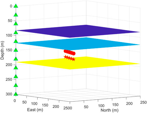
FIGURE 1. The layered anisotropic model used in synthetic tests. There are 11 receivers (green triangles) located in the monitoring well and two fracture systems in the third layer, which is associated with five microseismic events (red stars and red dots).

TABLE 1

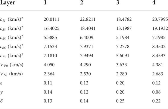
TABLE 1. The anisotropic parameters of the four layers.

As the data in microseismic is often not sufficient to pick all three waves (qP, qSV and SH), we discuss two cases that only the arrival times of P-wave are used or the arrival times of three wave types are all used in the joint inversion. For the application of field data, the initial guess of the anisotropic parameters is derived from the polarization analysis of the seismic data (Grechka et al., 2011). A least-squares objective function is constructed to invert the anisotropic model with a local isotropic assumption (Grechka and Mateeva, 2007). As we are only focusing on the sensitivity analysis in this study, the parameters of mentioned above are directly used with 5% randomly perturbation. In the analysis of specific cases, firstly the Fréchet derivatives (Eq. 6) is calculated and used as the input for SVD. Then the eigenvectors are sorted by their corresponding singular values. Then the element in the column are automatically sequenced by the maximum value and formed the suggested inversion strategy. With less parameter with singular values close to zero, the inversion process is better constrained.

First, we use the qP arrival times of ten microseismic event recorded by all receivers in sensitivity analysis. When the elastic moduli are used to represent the anisotropic media, the results are shown in Figure 2. The singular values close to zero indicates there are four parameters that can not be inverted. By resorting the rows to make it with best diagonal dominance, we can find that the smallest singular values correspond to $c_{66}$. They are poorly constrained as the arrival times of S- waves are not used.

FIGURE 2

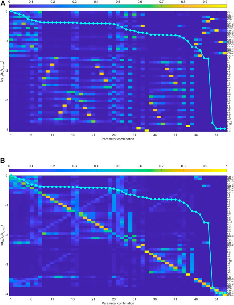
FIGURE 2. (A) The sensitivity analysis of the joint inversion using qP arrival times in the downhole array. The anisotropic is represented by $c_{ij}$ parametrization. (B) the rows of eigenvector matrix are sorted to make it diagonally dominant as possible. The horizontal axis shows the index of eigenvectors, the vertical axis on the left shows the corresponding normalized singular values, and the vertical axis on the right shows the represented parameters. The blue solid dotted line in (B) indicates the suggestion inversion sequence of the unknowns. The singular values close to zero means the parameters on the right do not contribute to the observed data.

When the initial model is close to the true solution, Figure 2B shows the methodology to invert the parameters in the downhole geometry shown in Figure 1. When only the arrival times of P- waves are used, the arrival times are strongly related with $c_{66}$, $c_{11}$, the radial distance $r$ and the vertical distance $h$. The values of layer thickness $l$ and the origin times $\tau$ have lower sensitivity to the arrival times. The value of $c_{13}$ is least constrained in the joint inversion. When only the arrival times of P-wave are available, the columns that have non-zero singular values have off-diagonal elements with high values. It indicates the crosstalk between the parameters are introduced and some trade-off exist. The parameter array on the right in Figure 2B shows the possible inversion sequence, from the best constrained parameter to the worst.

Figure 3 shows the result when the anisotropic media are represented by Thomsen-type parameters. In this case, the sensitivity analysis provided the relation sequence: $V_{P0}$, $\epsilon$, $r$, $h$, $\delta$, $l$ and $V_{S0}$. It has four near-zero singular values corresponding to $\gamma$ in the four layers, which means they can not be inverted in the joint inversion.

FIGURE 3

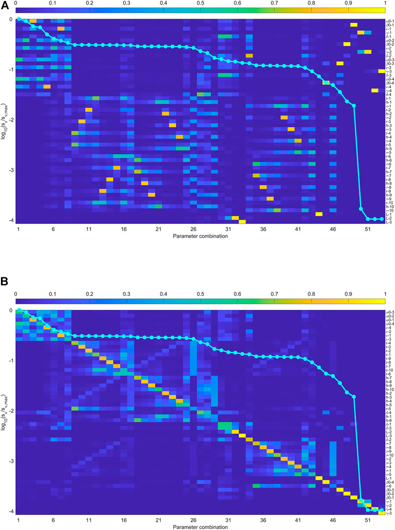
FIGURE 3. (A) The sensitivity analysis of the joint inversion using qP arrival times in the downhole array. The anisotropic is represented by Thomesen parametrization. (B) the rows of eigenvector matrix are sorted to make it diagonally dominant as possible. The singular values close to zero means the parameters on the right do not contribute to the observed data.

When the arrival times of three wave types are used, the anisotropic parameters are better constrained in the inversion. Figures 4, 5 show the result. Figure 4B indicates that $c_{55}$, $c_{66}$, $c_{13}$ and $c_{11}$ have the highest possibility to be inverted from the inversion. The second group is the radial and vertical distance $r$, $h$, and $c_{33}$. The similar colors of $r$ and $h$ in each column indicate that the two parameters trade-off with each other. The third group is the excitation time of ten events and the layer thickness. Figure 5B shows that the relation sequence becomes $V_{S0}$, $V_{P0}$, $\epsilon$, $\gamma$, $\delta$, $r$, $h$. The parameters that are not well constrained in the joint inversion are still the excitation times and layer thickness.

FIGURE 4

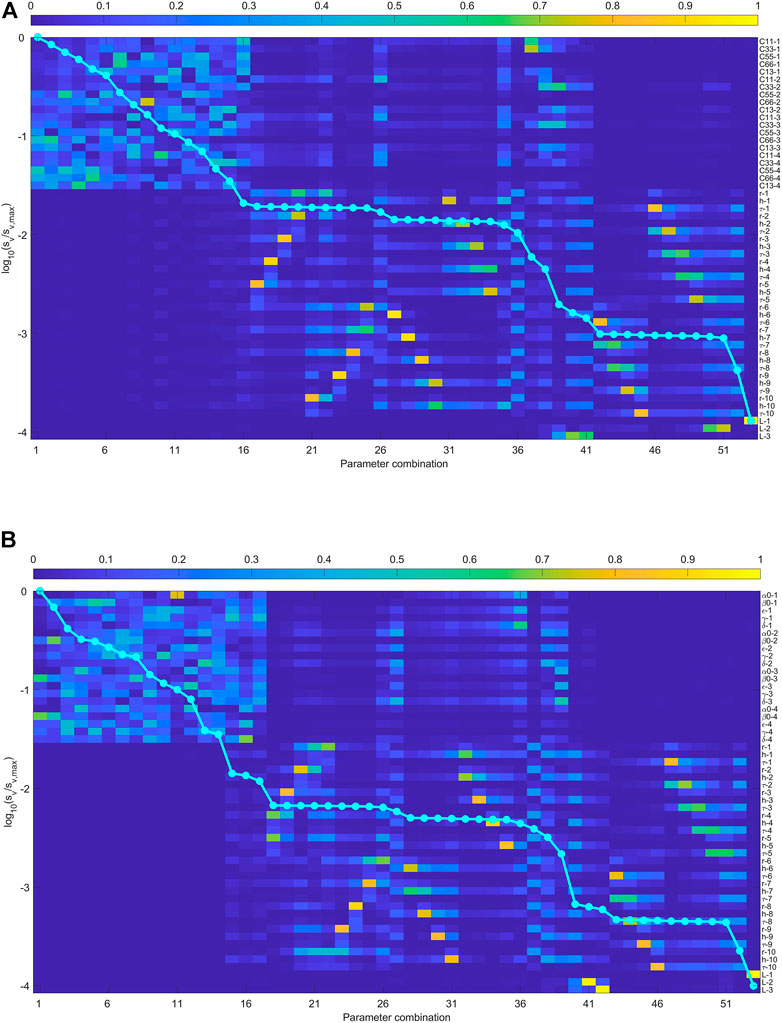
FIGURE 4. (A) The sensitivity analysis of the joint inversion using the arrival times of qP wave and two S- waves. The anisotropic is represented by $c_{ij}$ parametrization. (B) the rows of eigenvector matrix are sorted to make it diagonally dominant as possible. The absence of singular values close to zero means all the parameters on the right contribute to the observed data.

FIGURE 5

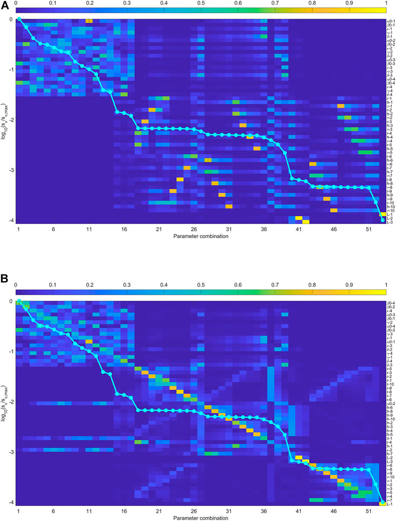
FIGURE 5. (A) The sensitivity analysis of the joint inversion using the arrival times of qP wave and two S- waves. The anisotropic is represented by Thomsen-type parametrization. (B) the rows of eigenvector matrix are sorted to make it diagonally dominant as possible. The absence of singular values close to zero means all the parameters on the right contribute to the observed data.

We used the downhole array to illustrate the proposed method, and it is also applicable to surface geometries or more mircoseismic events. The difference is the traveltimes calculation for the relative locations between receiver and microseismic sources. In the specific cases, the analysis process should be performed respectively and the terms in the derivatives need to be adjusted accordingly. The inferred inversion strategy highly depends on the locations of the events and receivers, but the main procedures are quite similar and not included here.

4 Conclusion

The sensitivity analysis of the joint inversion are obtained by the SVD of the Fréchet derivative matrix. As the monitoring arrays affect the measured quantities, this analysis should be done for each specific monitoring array. We use elastic moduli and Thomsen-type parametrization to describe the VTI media as the horizontal shale layers often have vertical axis of symmetry.

We derive the derivative of group velocity with respect to the elastic moduli and Thomsen-type parameters. We demonstrate how to establish the Fréchet derivative matrix in the joint inversion of anisotropic parameters and source locations. We show how to perform the sensitivity analysis to the monitoring array. It gives the tool to judge the constrain on the unknows in the joint inversion when limited data are obtained.

Data availability statement

The original contributions presented in the study are included in the article/Supplementary Material; further inquiries can be directed to the corresponding author.

Author contributions

YZ performed the data analysis. YW provided the research ideas and supervised the findings of this work. YZ and YW wrote and revised the manuscript.

Funding

This study was funded by the The Scientific Instrument Developing Project of the Chinese Academy of Sciences (Broadband fiber optic seismometer acquisition instrument and system), and Key Research Program of Frontier Sciences, Chinese Academy of Sciences (Grant No. QYZDY-SSW-DQC009).

Acknowledgments

We express our gratitude to Leo Eisner for the helpful discussions and comments.

Conflict of interest

The authors declare that the research was conducted in the absence of any commercial or financial relationships that could be construed as a potential conflict of interest.

Publisher’s note

All claims expressed in this article are solely those of the authors and do not necessarily represent those of their affiliated organizations, or those of the publisher, the editors and the reviewers. Any product that may be evaluated in this article, or claim that may be made by its manufacturer, is not guaranteed or endorsed by the publisher.

Supplementary material

The Supplementary Material for this article can be found online at: https://www.frontiersin.org/articles/10.3389/feart.2022.1023141/full#supplementary-material

References

Bardainne, T., and Gaucher, E. (2010). Constrained tomography of realistic velocity models in microseismic monitoring using calibration shots. Geophys. Prospect. 58 (5), 739–753. doi:10.1111/j.1365-2478.2010.00912.x

CrossRef Full Text | Google Scholar

Duncan, P. M., and Eisner, L. (2010). Reservoir characterization using surface microseismic monitoring. Geophysics 75 (5), 75A139–75A146. doi:10.1190/1.3467760

CrossRef Full Text | Google Scholar

Eisner, L., Duncan, P. M., Heigl, W. M., and Keller, W. R. (2009). Uncertainties in passive seismic monitoring. Lead. Edge 28 (6), 648–655. doi:10.1190/1.3148403

CrossRef Full Text | Google Scholar

Eisner, L., Zhang, Y., Duncan, P., Mueller, M. C., Thornton, M. P., and Gei, D. (2011). Effective VTI anisotropy for consistent monitoring of microseismic events. Lead. Edge 30 (7), 772–776. doi:10.1190/1.3609092

CrossRef Full Text | Google Scholar

Gei, D., Eisner, L., and Suhadolc, P. (2011). Feasibility of estimating vertical transverse isotropy from microseismic data recorded by surface monitoring arrays. Geophysics 76 (6), WC117–WC126. doi:10.1190/geo2011-0028.1

CrossRef Full Text | Google Scholar

Grechka, V. (2010). Data-acquisition design for microseismic monitoring. Lead. Edge 29 (3), 278–282. doi:10.1190/1.3353723

CrossRef Full Text | Google Scholar

Grechka, V., and Duchkov, A. A. (2011). Narrow-angle representations of the phase and group velocities and their applications in anisotropic velocity-model building for microseismic monitoring. Geophysics 76 (6), WC127–WC142. doi:10.1190/geo2010-0408.1

CrossRef Full Text | Google Scholar

Grechka, V., and Mateeva, A. (2007). Inversion of P-wave VSP data for local anisotropy: Theory and case study. Geophysics 72 (4), D69–D79. doi:10.1190/1.2742970

CrossRef Full Text | Google Scholar

Grechka, V., Singh, P., and Das, I. (2011). Estimation of effective anisotropy simultaneously with locations of microseismic events. Geophysics 76 (6), WC143–WC155. doi:10.1190/geo2010-0409.1

CrossRef Full Text | Google Scholar

Grechka, V. (2015). Tilted TI models in surface microseismic monitoring. Geophysics 80 (6), WC11–WC23. doi:10.1190/geo2014-0523.1

CrossRef Full Text | Google Scholar

Grechka, V., and Yaskevich, S. (2014). Azimuthal anisotropy in microseismic monitoring: A bakken case study. Geophysics 79 (1), KS1–KS12. doi:10.1190/geo2013-0211.1

CrossRef Full Text | Google Scholar

Huang, G., Ba, J., Du, Q., and Carcione, J. M. (2019). Simultaneous inversion for velocity model and microseismic sources in layered anisotropic media. J. Petroleum Sci. Eng. 173, 1453–1463. doi:10.1016/j.petrol.2018.10.071

CrossRef Full Text | Google Scholar

Kazei, V., and Alkhalifah, T. (2018). Waveform inversion for orthorhombic anisotropy with P waves: Feasibility and resolution. Geophys. J. Int. 213 (2), 963–982. doi:10.1093/gji/ggy034

CrossRef Full Text | Google Scholar

Li, J., Zhang, H., Rodi, W. L., and Toksoz, M. N. (2013). Joint microseismic location and anisotropic tomography using differential arrival times and differential backazimuths. Geophys. J. Int. 195 (3), 1917–1931. doi:10.1093/gji/ggt358

CrossRef Full Text | Google Scholar

Li, L., Tan, J., Schwarz, B., Staněk, F., Poiata, N., Shi, P., et al. (2020). Recent advances and challenges of waveform-based seismic location methods at multiple scales. Rev. Geophys. 58 (1), e2019RG000667. doi:10.1029/2019RG000667

CrossRef Full Text | Google Scholar

Li, L., Tan, J., Wood, D. A., Zhao, Z., Becker, D., Lyu, Q., et al. (2019b). A review of the current status of induced seismicity monitoring for hydraulic fracturing in unconventional tight oil and gas reservoirs. Fuel 242, 195–210. doi:10.1016/j.fuel.2019.01.026

CrossRef Full Text | Google Scholar

Li, L., Tan, J., Xie, Y., Tan, Y., Walda, J., Zhao, Z., et al. (2019a). Waveform-based microseismic location using stochastic optimization algorithms: A parameter tuning workflow. Comput. Geosciences 124, 115–127. doi:10.1016/j.cageo.2019.01.002

CrossRef Full Text | Google Scholar

Maxwell, S. C., Rutledge, J., Jones, R., and Fehler, M. (2010). Petroleum reservoir characterization using downhole microseismic monitoring. Geophysics 75 (5), 75A129–75A137. doi:10.1190/1.3477966

CrossRef Full Text | Google Scholar

Michel, O. J., and Tsvankin, I. (2016). “Anisotropic waveform inversion for microseismic velocity analysis and event location,” in SEG technical Program expanded abstracts 2016 (Texas United States: Society of Exploration Geophysicists), 296–300.

CrossRef Full Text | Google Scholar

Pan, X., Du, X., Zhao, X., Ge, Z., Li, L., Zhang, D., et al. (2022). Seismic characterization of decoupled orthorhombic fractures based on observed surface azimuthal amplitude data. IEEE Trans. Geosci. Remote Sens. 60, 1–12. doi:10.1109/TGRS.2021.3105724

CrossRef Full Text | Google Scholar

Pei, D., Quirein, J. A., Cornish, B. E., Quinn, D., and Warpinski, N. R. (2009). Velocity calibration for microseismic monitoring: A very fast simulated annealing (vfsa) approach for joint-objective optimization. Geophysics 74 (6), WCB47–WCB55. doi:10.1190/1.3238365

CrossRef Full Text | Google Scholar

Thomsen, L. (1986). Weak elastic anisotropy. Geophysics 51 (10), 1954–1966. doi:10.1190/1.1442051

CrossRef Full Text | Google Scholar

Thurber, C. H. (1986). Analysis methods for kinematic data from local earthquakes. Rev. Geophys. 24 (4), 793–805. doi:10.1029/rg024i004p00793

CrossRef Full Text | Google Scholar

Tsvankin, I. (2012). Seismic signatures and analysis of reflection data in anisotropic media. Texas United States: Society of Exploration Geophysicists.

Google Scholar

Zhang, H., and Thurber, C. H. (2003). Double-difference tomography: The method and its application to the Hayward fault, California. Bull. Seismol. Soc. Am. 93 (5), 1875–1889. doi:10.1785/0120020190

CrossRef Full Text | Google Scholar

Zhang, J., and Toksoz, M. N. (1998). Nonlinear refraction travel time tomography. Geophysics 63, 1726–1737. doi:10.1190/1.1444468

CrossRef Full Text | Google Scholar

Zhou, B., and Greenhalgh, S. A. (2005). Analytic expressions for the velocity sensitivity to the elastic moduli for the most general anisotropic media. Geophys. Prospect. 53 (4), 619–641. doi:10.1111/j.1365-2478.2005.00490.x

CrossRef Full Text | Google Scholar

Zimmer, U., Bland, H., Jing, D., Warpinski, N., Sen, V., and Wolfe, J. (2009). “Accuracy of microseismic event locations recorded with single and distributed downhole sensor arrays,” in SEG technical Program expanded abstracts. Houston, TX: Society of Exploration Geophysicists. 1519–1523.

CrossRef Full Text | Google Scholar