Seismicity-based 3D model of ruptured seismogenic faults in the North-South Seismic Belt, China

The North–South Seismic Belt produces the most frequent strong earthquakes in the Chinese continental region, such as the MS 8.0 Wenchuan earthquake on 12 May 2008 and Ms 7.0 Lushan earthquake on 20 April 2013. This seismicity results in significant hazards. Fault geometry modeling is crucial for analyzing earthquake preparation and trigger mechanisms, simulating and predicting strong earthquakes, inverting fault slip rates, etc. In this study, a novel method for obtaining geometric models of ruptured seismogenic faults over a large area is designed based on datasets from surface fault traces, fault orientations, focal mechanism solutions, and earthquake relocations. This method involves three steps. 1) An initial model of the fault geometry is constructed from the focal mechanism solution data. This initial model is used to select the earthquake relocation data related to the target fault. 2) Next, a fine model of the fault geometry with a higher resolution than that of the initial model is fitted based on the selected earthquake relocation data. 3) The minimum curvature interpolation method (Briggs, 2012) is adopted to build a 3D model of the subsurface fault geometry according to the three-dimensional coordinates of nodes on all profiles of each fault/segment. Based on this method and data collected in the North–South Seismic Belt, the fine morphologies of different faults along 1,573 transverse profiles were fitted, and a 3D model of 263 ruptured seismogenic faults or fault segments in the North–South Seismic Belt was built using the minimum curvature spatial interpolation method. Since the earthquake number decreases with increasing depth, the model uncertainty increases with increasing depth. Different ruptured faults have different degrees of seismicity, so different fault models may have different uncertainties. The overall fitting error of the model is 0.98 km with respect to the interpreted results, from six geophysical exploration profiles.

1 Introduction

As the region with the most frequent strong earthquakes in the Chinese mainland, the North–South Seismic Belt (NSSB) extends more than 800 and 2,000 km in the east-west and north-south directions, respectively (Figure 1) (Wang et al., 2015). The NSSB has generated numerous strong earthquakes that have caused significant hazards, such as the MS 8.0 Wenchuan earthquake on 12 May 2008, Ms 7.0 Lushan earthquake on 20 April 2013, MS 6.4 Yangbi earthquake on 21 May 2021, and Ms 6.8 Luding earthquake on 5 September 2022 (Dai et al., 2011; Zhou et al., 2015; Yang et al., 2022). This seismic belt extends from the western margin of the Ordos Block in the north, crosses the Qinling Orogenic Belt and Longmenshan Fault Belt, and reaches Myanmar along the Anninghe Fault (ANH. F.) (Figure 1). The relatively stable South China Block and Ordos Block in the eastern Chinese mainland are separated from the Qinghai-Tibetan Plateau in the west by the NSSB (Zhang, 2013). The NSSB is the region of interactions among the Sichuan–Yunnan Block, Bayankala Block, Qinling Orogenic Belt, East Kunlun Orogenic Belt, Qaidam-Longxi Block, Qilian Orogenic Belt, Ordos Block, and Alxa Block (Figure 1) (Zhang et al., 2015).

FIGURE 1

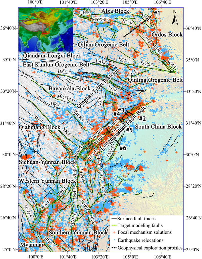
FIGURE 1. Tectonic setting and basic data distribution for fault modeling in the North–South Seismic Belt, China. ETOPO1 (Amante, 2009) is used as the topographic base map. The black solid lines represent the surface fault traces, (Xu et al., 2016), which contain 263 faults (segments): Y-B. F., Yingxiu-Beichuan Fault; G-A. F., Guanxian-Anxian Fault; W-W. F., Wenchuan-Wenmao Fault; XSH. F., Xianshuihe Fault; ZMH. F., Zemuhe Fault; ANH. F., Anninghe Fault; HH. F., Honghe Fault; DKL. F., Dongkunlun Fault; YK. F., Yuke Fault; JPS. F., Jinpingshan Fault; L-X. F., Lijiang-Xiaojinhe Fault; E-J. F., Ebian-Jinyang Fault; XJ. F., Xiaojiang Fault; DR. F., Dari Fault; HY. F., Haiyuan Fault; L-D. F., Lintan-Dangchang Fault; L-L. F., Lixian-Luojiabao Fault; LQS. F., Longquanshan Fault; MEK. F., Malkan Fault; MJ. F., Minjiang Fault; TZ. F., Tazang Fault; XQL. F., Xiqinling Fault. The green dashed lines represent the faults whose subsurface geometries are modeled in this study. The red crosses represent the positions of focal mechanism solutions (Zheng, 2019; Guo et al., 2022). The blue dots represent the relocated epicenters of earthquakes from the Sichuan Earthquake Administration. The black dotted lines represent geophysical exploration profiles: #1, an electrical structure profile across the Haiyuan Fault (Min, 2014); #2, a seismic profile across the Yingxiu-Beichuan Fault and Guanxian-Anxian Fault (Dong et al., 2010); #3, a seismic profile across the Yingxiu-Beichuan Fault (Wu et al., 2014); #4, a seismic profile across the Yingxiu-Beichuan Fault (Wu et al., 2014); #5, a seismic profile across the Yingxiu-Beichuan Fault and Guanxian-Anxian Fault (Dong et al., 2010); #6, a seismic profile across the Longquanshan Fault (Dong et al., 2010).

Seismological studies in the NSSB are of great significance, and three-dimensional models of ruptured seismogenic faults are the basis for several seismological studies. For example, fault geometric models can be used for the inversion of fault slip rates (Li et al., 2010; Wang et al., 2016; Liu et al., 2022), the analysis of seismogenic mechanisms (King, 1986; Barka and Kadinsky-Cade, 1988; Shi et al., 2019) and seismic triggering mechanisms (Lay et al., 2010; Mildon et al., 2019; Ross et al., 2019), the prediction and simulation of strong earthquakes (Silva and Vitor., 2016; Walker et al., 2019; Xin and Zhang, 2021), etc. At present, the geometries of ruptured seismogenic faults are imaged mainly by field geological surveys, active-source geophysical surveys, seismic tomography based on passive earthquake data, and earthquake parameter estimation.

However, subsurface fault shapes cannot be identified by surface geological surveys (Valoroso et al., 2014). Active-source geophysical surveys always have with low data coverage due to their high cost (Hubbard and Shaw, 2009; Dong et al., 2010; Li Y. et al., 2019). For seismic tomography, the resolution of data depends on the distribution of seismic rays (Dorbath et al., 1996; Dilla et al., 2018). Unevenly distributed hypocenters and limited seismic stations result in low-resolution seismic tomography (Liu et al., 2021; Zhao et al., 2021).

There are two independent methods for modeling ruptured seismogenic faults based on earthquake parameters. One method is based on hypocenters, and the other method is based on focal mechanism solutions. In the first method, the fault geometry is fitted by the distribution of hypocenters along a fault based on the relationship between the rupture area of the ruptured seismogenic fault and the magnitude of the earthquakes, as well as the attenuation of seismic wave energy (Wells and Coppersmith, 1994; Lin et al., 2007; Schaff and D., 2009). In subduction zones, the majority of earthquakes are located along the Benioff zone, so the plate boundary can be modeled based on hypocenter fitting. The slab surfaces at the main subduction zones on Earth have been obtained via this method (Hayes and Wald, 2009; Zhang et al., 2013). However, an initial or coarse model of fault geometry is necessary to select the earthquakes induced by the target fault when modeling the geometry of small-scale ruptured seismogenic faults because some earthquakes near the target fault may be triggered by the other faults (Schaff et al., 2002; Hayes and Wald, 2009). The 3D geometry of the Gualdo Tadino Fault in Italy was fitted based on aftershock relocations, which were selected based on the constraints of seismic reflection profiles (Ciaccio et al., 2005). A three-dimensional model of the Longmenshan Fault in China was built based on the surface ruptures and aftershock relocations due to the Wenchuan earthquake in 2008, and the hypocenters used in the fitting process were also selected under the constraints of a deep seismic-reflection profile and logging data (Li et al., 2010).

In the focal mechanism solution-based method, the fault geometry can be modeled by the dip variations estimated from focal mechanism solutions at different depths, according to the relationship between seismic wave propagation and the rupture process of ruptured seismogenic faults (Aki, 1966; Nolet, 1980; Sliver et al., 1982; Kuang et al., 2021). The variations in the dip of the rupture planes of a fault were mapped according to 24 focal mechanism solutions in the western Corinth Rift in Greece (Maxime et al., 2014). Frepoli et al. (2017) also inferred the dip angle of Apennine faults in central Italy based on focal mechanism solutions. Duan et al. (2018a) estimated the dip variations along the Dujiangyan Fault in the NSSB of China based on focal mechanism solutions. However, the number of focal mechanism solutions is always much lower than the amount of earthquake relocation data due to the limited number of seismic stations. Therefore, compared with a fault model based on earthquake relocations, a model based on focal mechanism solutions often has a lower resolution, which cannot reflect the detailed fault geometry (Ciaccio et al., 2005; Frepoli et al., 2017).

By integrating surface traces, focal mechanisms, earthquake relocations, logging data, and seismic reflection profiles, a three-dimensional fault model was developed for southern California in the United States (Plesch et al., 2007). Similarly, a three-dimensional fault model was built for the main ruptured seismogenic faults in the Sichuan–Yunnan region under the comprehensive constraints of fault traces, focal mechanism solutions, precise locations of small earthquakes, a crustal velocity model, seismic reflection profiles, and magnetotelluric data; this work was accomplished by the China Seismic Experimental Site project (http://www.cses.ac.cn/). However, this model does not cover the whole NSSB, and some major faults in this seismic belt, such as the Haiyuan Fault, Xiangshan-Tianjingshan Fault, and Weihe Fault (Lu et al., 2019), are not included. At present, a 3D fault geometric model that covers the whole NSSB is still lacking.

The coverage of active-source geophysical profiles in the NSSB, such as electrical, magnetic and seismic profiles, are very limited. Therefore, these geophysical interpretations cannot be taken as constraints for relocation data selection. In this study, the initial model of fault geometry is modeled based mainly on the focal mechanism solutions and partly on the available geological and geophysical data. The detailed shapes of the ruptured seismogenic faults are modeled by fitting the selected hypocenters according to the initial model. Finally, we evaluate the uncertainty of the fault model based on the six geophysical exploration profiles.

2 Data and methods

2.1 Input data

The necessary input data for 3D modeling of the main ruptured seismogenic faults in the NSSB include fault traces on the Earth’s surface, fault orientations, focal mechanism solutions, and relocated hypocenters. The fault orientations and focal mechanism solutions are used to construct the initial fault geometry model and choose relocated hypocenters related to the target fault. The selected relocated hypocenters are used to fit the fault geometry. In addition, geophysical interpretation profiles are also necessary to test the model uncertainty.

1) The surface trace of each fault (Figure 1) is extracted from the Seismotectonic Map of China and Adjacent Regions compiled by Xu et al. (2016), which is provided by the Data Exchange and Sharing Management Center of Active Fault Exploration in the Institute of Geology, China Earthquake Administration.

2) The fault orientations are derived from seismic, electrical and magnetic exploration. These data are compiled and provided by the Sichuan Earthquake Administration, China.

3) The focal mechanism solutions are from the National Earthquake Data Sharing Project by the China Earthquake Administration (Zheng, 2019) and the Focal Mechanism Data Set of the Chinese Mainland and Its Adjacent Areas (2009–2021), which was compiled by the Institute of Geophysics, China Earthquake Administration (Guo et al., 2022). There are 7,427 focal mechanism solutions within the NSSB in this study (Figure 1).

4) The earthquakes relocations are from the catalog of the China Seismic Experimental Site (http://www.cses.ac.cn/), including the relocated hypocenters of 127,009 earthquakes with magnitudes larger than ML 1.5 in the NSSB from January 2009 to March 2019 (Figure 1). These relocations are derived by the Sichuan Earthquake Administration using absolute and relative earthquake location methods based on the seismic phase observed by the seismic networks in the NSSB. The uncertainties of these relocated hypocenters are given as follows: the root mean square (RMS) of the travel times for 80% of the earthquakes is within 0.3 s, the horizontal error for 80% of the samples is limited to 2 km, and the vertical error for 80% of the samples is within 4 km, which are the statistics based on absolute earthquake locations.

5) Fault interpretation results along six geophysical profiles across different faults (Figure 1) are collected. The details of these profiles are listed in Table 1.

TABLE 1

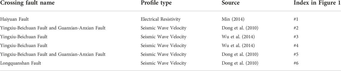
TABLE 1. Information on the six collected geophysical profiles in the NSSB.

2.2 Modeling method

The geometric and kinematic parameters of ruptured seismogenic faults can be indicated well by focal mechanism solutions (Ciaccio et al., 2005; Frepoli et al., 2017), and earthquakes are mainly concentrated on ruptured seismogenic faults (Schaff et al., 2002; Hayes and Wald, 2009). Therefore, the geometry of a ruptured seismogenic fault can be modeled based on focal mechanism solutions and earthquake relocations. Our modeling method includes three main steps (Figure 2). 1) First, an initial fault model with a coarse resolution is constructed along the fault strike based on the focal mechanism solution, surface fault trace the collected fault orientation. 2) The relocated hypocenters of earthquakes due to the specific ruptured seismogenic fault are selected under the constraint of the initial fault model. The fault geometries along different cross-sections (the solid black line in Figure 3C) that are perpendicular to the fault strike are fitted based on the relocation data. 3) A three-dimensional model of the fault geometry is built by compiling all the fault shapes along different fault-crossing profiles.

FIGURE 2

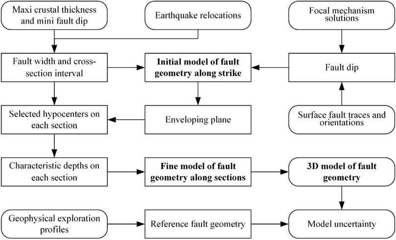
FIGURE 2. The workflow of 3D fault geometry modeling. The main stages are as follows: 1) the potential maximum fault width is derived from the maximum crustal thickness and minimum fault dip in the research region. The more precise fault width can be judged according to the distributions of the relocated hypocenters within the maximum fault width. The fault dip variations are gridded within the judged fault width based on the dips reflected by the nodal planes of focal mechanism solutions which are selected according to the surface fault traces and orientations. The low-resolution initial model of fault geometry along fault strike is constructed according to the fault dip variations. 2) The cross-section interval along each fault strike is evaluated by setting relocated hypocenter number is not less than 200 on each section within fault width. The hypocenters within the enveloping plane, which is with the highest hypocenter density, is used to calculate the characteristic depths on each section. The high-resolution fine fault geometry along each cross-section is modeled by fitting the characteristic depths. 3) The 3D fault geometry is modeled based on the fine geometries along different sections, and the uncertainty of the 3D model is estimated by taking the fault geometries from geophysical interpretation results as references.

FIGURE 3

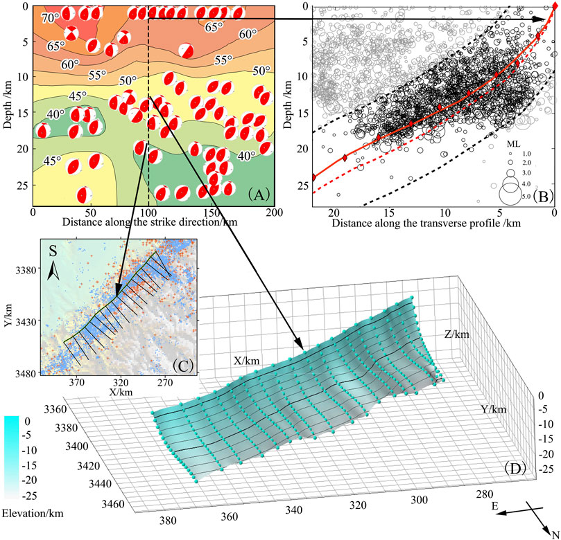
FIGURE 3. Three-dimensional modeling process for subsurface geometry taking the middle segment of the Yingxiu-Beichuan Fault as an example. (A) Fault dip variations according to the focal mechanism solutions; (B–C) Fine model of fault geometry along profile by fitting the selected and relocated hypocenters; (D) 3D model of the fault plane.

2.2.1 Initial model of fault geometry along strike

To construct the fault model, the width of the fault along each fault strike-orthogonal profile needs to be delineated to extract the focal mechanism solutions and the relocated hypocenters, which are the basis for fault geometry modeling. The width of the fault is estimated through the following two steps. 1) According to the maximum crustal thickness (70 km) of the NSSB (Chen et al., 2015; Wang et al., 2017) and the minimum dip (30°) of the modeled faults, the maximum width of the fault is set to 120 km based on the trigonometric function. In this way, all the potential seismicity data related to the target fault should be within this maximum fault model width. 2) Then, a bounding region that covers the target fault can be judged according to the intensity of the relocated hypocenter distribution because the seismicity decreases with distance from the target ruptured seismogenic fault. The approximate shape of the target fault can be inferred by combining the fault orientations and the dip angle reflected by the majority of the focal mechanism solutions. The abscissa spanning between the surface outcrop point and the other intersection point between the bounding region and the fault model is regarded as the width of the target fault, which can be modeled according to seismicity data. While ensuring that the width is not underestimated, this process also eliminates the need to introduce the seismicity data of adjacent faults because of setting an overly large width.

The focal mechanism solutions are extracted within this width. Based on the fault strike according to the surface traces, the proper nodal plane can be chosen from the focal mechanism solution. The focal mechanism solutions, which clearly differ from the main trend and are probably caused by the other adjacent ruptured seismogenic faults, are removed from the dataset. The percentages of the removed focal mechanism solutions at different profiles vary, ranging between 10% and 20%. The gridded fault dip variations along the fault plane are interpolated according to the dips based on the extracted focal mechanism solutions via the kriging interpolation method. The grid size ($c$) is estimated by the following equation (Hengl, 2006):

$c=0.25\sqrt{\frac{A}{N},}(1)$

where $A$ is the area of the fault plane and $N$ is the number of focal mechanism solutions. Finally, the initial model of the fault geometry can be derived based on the fault dip variations along the fault plane.

2.2.2 Fine model of fault geometry along cross-sections

Relative to the initial model in the former step, the fine model of the fault geometry is based on fitting the relocated hypocenters along different fault-strike-orthogonal profiles. These profiles have the same interval along the fault strike. A small cross-section interval means a high model resolution along strike, but it also means few earthquake relocations and a low vertical resolution for the fault geometry along each profile. Therefore, to obtain a fault model with enough details in both the horizontal and vertical directions based on the finite number of relocated hypocenters, we should balance the number of cross-sections and that of earthquake relocations on each profile. The profile length is determined by the horizontal width of the initial model of fault geometry. According to our multiple tests, one suitable choice is that the minimum number of earthquake relocations along each profile is 200. Based on this condition, the profile interval along strike and the profile number can be obtained when the minimum number of earthquake relocations along each profile is slightly larger than 200. When there are not more than 200 relocated hypocenters related to one fault, the fault geometry is fitted along only one profile at the fault center and orthogonal to the strike. Then, the three-dimensional fault model is derived by extending this along-profile geometry according to the surface trace.

To fit the detailed fault shape along one profile, the relocated earthquake hypocenters within the region surrounded by two neighboring profiles are extracted. Then, an enveloping plane (the black dashed lines in Figure 3B) is constructed by taking the initial model line as the symmetry axis (the red dashed line in Figure 3B). To obtain enough relocated hypocenters whose source earthquakes are related to the target fault and to exclude as many hypocenters not related to the target fault as possible, this envelope should have as high a hypocenter density and as large an area as possible. The density of the relocated hypocenters in the envelop region usually first increases and then decreases with increasing envelope width because the earthquakes caused by fault activity are located near the fault plane. Therefore, the envelope with the maximum relocated hypocenter density is the optimal one. In particular, when there are other active faults near the target fault, hypocenters associated with other faults should be artificially removed.

The depths of nodes with equal intervals along the initial model of fault geometry are fitted based on the selected hypocenters. The spacing of nodes is taken as 2.5 km (Zhang et al., 2013; Duan et al., 2018b). The characteristic depth of each node is estimated by the weighted average method (Zhang et al., 2013), which can be expressed as:

$Z_{\left(x\right)}={\displaystyle \sum }_{i=1}^{i=n}\left(\frac{{\Omega }_i{\mu }_i}{{\displaystyle \sum }_{i=1}^{i=n}{\Omega }_i}\right),(2)$

where $Z_{\left(x\right)}$ is the characteristic depth of the $x$-th node, $n$ is the number of earthquake relocation data on the profile, ${\mu }_i$ is the focal depth of the $i$-th earthquake, and ${\Omega }_i\left(M_i,x_i\right)$ is the weight of the $i$-th earthquake. According to the relationship between earthquake magnitude and the main rupture plane area of the fault (Wells and Coppersmith, 1994) and the attenuation law of seismic waves (Winkler and Nur, 1982), the weight ${\Omega }_i\left(M_i,x_i\right)$ can be estimated by the following equation (Zhang et al., 2013):

${\Omega }_i={10}^{M_i}\exp \left(-\frac{{\left(x-x_i\right)}^2}{2D}\right),(3)$

where $x$ is the abscissa of the target node, $x_i$ is the abscissa of the $i$-th earthquake relocation on the profile, $M_i$ is the magnitude of the earthquake, and $D$ is the interval of the cross-sections on the fault. The estimated final positions of nodes are shown as solid diamonds in Figure 3B. The use of 2-4 order polynomial fitting is suggested, and the cubic polynomial is the most widely adopted one in similar modeling research (Hayes et al., 2009; Zhang et al., 2013; Duan et al., 2018b). Therefore, we also apply a cubic polynomial to fit all the nodes along the profile to refine the model of fault geometry (the solid red line in Figure 3B), and reliability of it is establish by comparing the effect of 2-4 order polynomial fitting in the 3.2 uncertainty and discussion.

2.2.3 Three-dimensional model and its uncertainty of fault geometry

Some of the faults are composed of different segments according to the surface traces. In this case, the unit of the three-dimensional fault geometry modeling is the fault segment. Otherwise the unit is the whole fault. Then, the minimum curvature interpolation method (Briggs, 2012) is adopted to build the 3D model of the subsurface fault geometry according to the three-dimensional coordinates of nodes on all profiles of each fault/segment. The uncertainty of this 3D model is estimated by comparing the modeled fault geometry with the published fault geometry, where the latter is based on active-source geophysical explorations. The fault depth differences between our model and the reference result at the points along the profile with a constant horizontal interval are used to estimate the root mean square error (RMSE) of our model. The RMSE can be calculated as follows:

$\mathrm{R}\mathrm{M}\mathrm{S}\mathrm{E}=\sqrt{\frac{{\displaystyle \sum }_{i=1}^n{\left(y_i-y_i^{\prime }\right)}^2}{n}},(4)$

where $y_i$ and $y_i^{\prime }$ are the fault plane depth at the $i$-th point from our model and the reference result, respectively, and $n$ is the number of comparison points. A smaller RMSE means a smaller uncertainty in our fitted fault model.

3 Results and discussion

3.1 3D model of ruptured seismogenic faults in the NSSB

The middle segment of the Yingxiu-Beichuan Fault is taken as an example to illustrate the fault modeling steps and selection of some parameters. Previous studies suggest that the fault dip angle is between 50° and 70° here, and the strike ranges from 210° to 230° (Lei and Zhao, 2009; Li et al., 2013; Nie et al., 2013; Si et al., 2014; Wang et al., 2014; Li et al., 2016; Meng et al., 2020). According to these conditions, 67 focal mechanism solutions in total are selected for this fault section, as shown in Figure 3A. Finally, the along-strike initial geometric model of the middle section of the Yingxiu-Beichuan Fault is modeled by interpolation of these focal mechanism solutions (Figure 3A).

In total, 18transverse profiles perpendicular to the middle segment of the Yingxiu-Beichuan Fault are constructed with a 10-km interval (Figure 3C). On average, 425 hypocenters are distributed along each profile, with a maximum of 926 and a minimum of 237. The central profile (Figure 3B) is selected to show the modeling results. The envelope region is 9 km wide; in other words, the distance between the upper and bottom black dashed lines in Figure 3B is 9 km. There are nine calculation nodes with an interval of 2.5 km whose characteristic depths (the red solid diamonds in Figure 3B) are fitted by 926 relocated hypocenters (the black hollow circle in Figure 3B), and the maximum burial depth of this fine model (red solid line in Figure 3B) is 23.8 km. Finally, the three-dimensional fault plane model (Figure 3D) of the middle segment of the Yingxiu-Beichuan Fault is obtained based on the fine models of fault geometry along the 18 transverse profiles (the solid black line in Figure 3C).

To model the 3D geometries of the 263 main ruptured seismogenic faults (fault segments) in the NSSB, the fine fault shapes along a total of 1,573 transverse profiles are fitted. The final 3D model covers all the main ruptured seismogenic faults, such as the Yingxiu-Beichuan Fault, Xianshuihe Fault, and Haiyuan Fault (Figure 4). The fitted fault length at the Earth’s surface, the number of fitted cross-sections, the maximum depth of the fault model, and some other parameters of the main faults in the 3D model are listed in Table 2; the detailed statistics are reported in Supplementary Table A1.

FIGURE 4

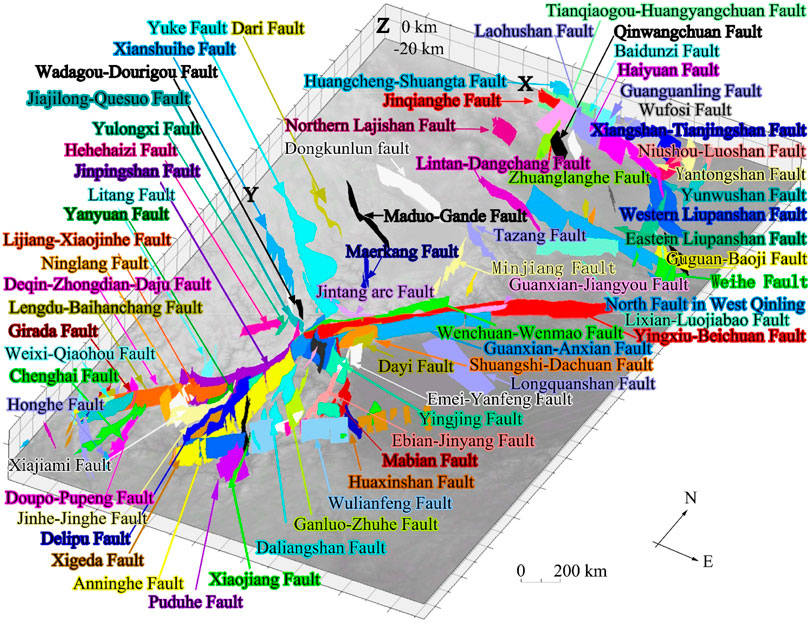
FIGURE 4. Oblique view of the 3D model of 263 ruptured seismogenic faults in the North–South Seismic Belt. ETOPO1 (Amante, 2009) is used as the base map and placed at a depth of 20 km, and the vertical exaggeration is 3X.

TABLE 2

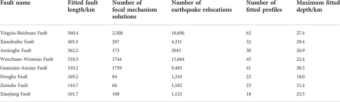
TABLE 2. Geometry modeling parameters for the main faults.

3.2 Uncertainty and discussion

Uncertainty is mainly caused by two aspects in our ruptured seismogenic fault geometry model, on the one hand, the uncertainty is determined by the order of polynomial used to fit the characteristic depth, on the other hand, is caused by the input data. For the former, the effect of 2-4 order polynomial fitting has been tested, the overall fitting error of them are 1.47 km, 0.98 km and 1.00 km respectively comparing geophysical interpretation results (Table 3). Comparatively, the 2 order polynomial is the worst, the 3 order is the best, and the fitting effects of the 3 order and 4 order polynomials are similar.

TABLE 3

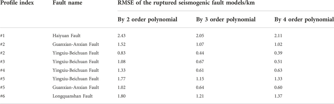
TABLE 3. The RMSE between the geophysical interpretation results and the fitting results based on 2−4 order polynomial by the method of this study.

As for the latter, there are different uncertainties such as the uncertainties in the focal mechanism solutions and the relocated hypocenters, and the number of hypocenters related to other faults used in the modeling. According to statistics, the focal mechanism solutions and relocated hypocenters used in this study decrease in number with increasing depth below a specific depth (Figure 3B). Fewer relocated hypocenters at the fault bottom means that the weight of the relocated hypocenters on the upper part becomes higher (Eq. 3), so the fitted node depth at the fault bottom will be shallower than that in reality. This process trends to yield listric fault models (Figures 5, 6). Therefore, the uncertainty at the bottom of the model tends to be larger than that of the shallow part (Figures 5, 6). The qualities of seismicity data also vary among different cross-sections or along different faults, so the model uncertainty also varies along strike or between different faults (Table 4). In addition, it is impossible to remove all the relocated hypocenters related to other faults based on the initial fault model, even though we attempt to do so. Therefore, this incomplete removal also introduces uncertainty to the fault geometry models.

FIGURE 5

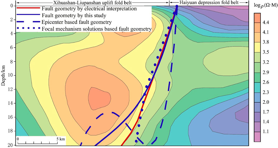
FIGURE 5. Comparison between the Haiyuan Fault geometry obtained from a geophysically interpreted profile (Min, 2014) and the three kinds of fitting results based on earthquake data. The electrical structure (Min, 2014) is taken as the base map.

FIGURE 6

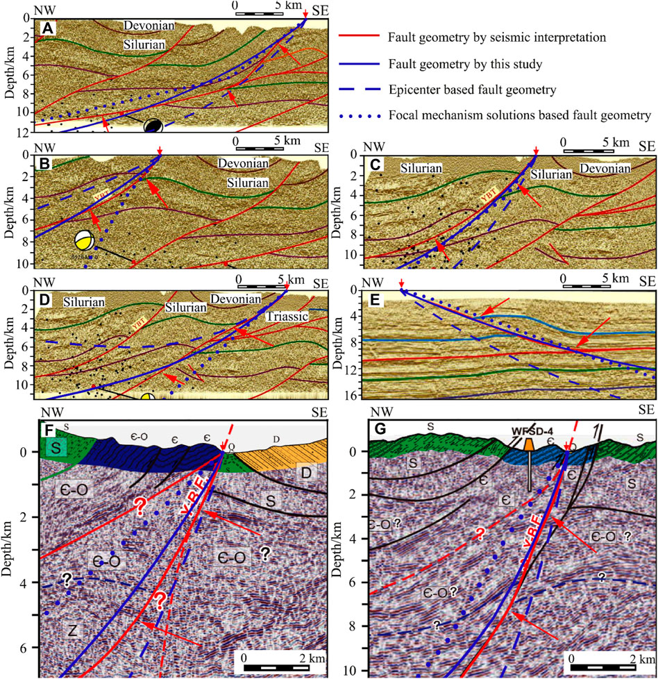
FIGURE 6. Comparison between the fault geometries obtained from seismic interpretation and the fitting results based on earthquake data. (A,B) are from Profile #2 (Dong et al., 2010); (C,D) are from Profile #5 (Dong et al., 2010); (E) is from Profile #6 (Dong et al., 2010); (F) is from Profile #4 (Wu et al., 2014); and (G) is from Profile #3 (Wu et al., 2014).

TABLE 4

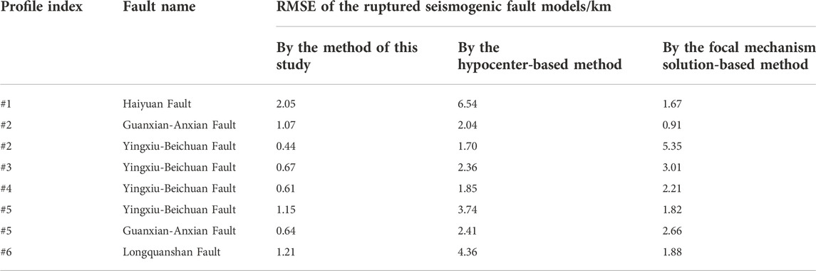
TABLE 4. The RMSE between the geophysical interpretation results and the fitting results based on different methods.

The uncertainty of the three-dimensional ruptured seismogenic fault model in the NSSB is estimated by taking the fault geometries from the six collected geophysical interpretation profiles as the reference. The RMSEs of the 3D model are shown in Table 4. Since the fault model can also be constructed based only on focal mechanisms, which is the same as our initial model of fault geometry, or only by fitting hypocenters along the profile without earthquake selection, Table 4 also provides the RMSEs of the fault model when using these two simplified methods. Among the three modeling methods, the approach designed in this study derives the smallest RMSE overall, which is 0.98 km. The fault geometries based on geophysical profile interpretations and the three different fitting methods are plotted on the geophysical profiles (Figures 5, 6). The comparison results suggest that the method of this study can best match the geophysical interpretation results among the three kinds of fitted results in most cases.

4 Conclusion

A new method for 3D modeling of ruptured seismogenic fault geometry based on seismicity is designed in this study. The focal mechanism solutions related to the target ruptured seismogenic fault are chosen by comparing their internal consistency or the consistency of each with the collected fault orientations, and the selected solutions are used to construct the initial model of fault geometry. The initial geometric model is further adopted to determine the earthquake relocation data related to the target fault. Subsequently, these earthquake relocations are employed to refine the fault model. This method can avoid the disadvantage of constructing only a low-resolution fault model when using focal mechanism solutions alone due to the limited amount of data. Moreover, it can also reduce the modeling uncertainty by removing the ambiguity of hypocenters with respect to other nearby fault or faults under the constraint of the initial geometric models.

Combining the surface traces of ruptured seismogenic faults in the NSSB, the initial geometric models of 263 faults (segments) are modeled based on the focal mechanism solutions under the constraints of prior data on fault orientations obtained from seismic, electrical and magnetic exploration. Moreover, detailed fault geometries along a total of 1,573 strike-perpendicular profiles are fitted based on the selected hypocenters. Finally, the minimum curvature interpolation method is adopted to build a three-dimensional model for the ruptured seismogenic faults in the NSSB. When taking six geophysical interpretation profiles as a reference, the average RMSE of this model is 0.98 km which is smaller than those of the other two traditional methods. The model uncertainty at the bottom is higher than that near the top because of the limited number of earthquakes, and the uncertainties for different sections of each fault may also differ because of the unevenly distributed earthquake data.

Data availability statement

The datasets presented in this study can be found in online repositories. The names of the repository/repositories and accession number(s) can be found in the article/Supplementary Material.

Author contributions

YR: Methodology, Validation, Modeling, Writing - Original Draft, Writing—Review Editing YB: Conceptualization, Methodology, Validation, Formal analysis, Writing—Original Draft, Writing—Review Editing MR: Modeling, Writing—Review Editing ML: Data providing, Writing—Review Editing ZW: Writing—Review Editing All authors contributed to manuscript revision, read, and approved the submitted version.

Funding

This study was supported by the National Key Research and Development Program of China (Grant No. 2019YFC1509204), the National Natural Science Foundation of China (No. 42176068), the Natural Science Foundation of Shandong, China (No. ZR2020MD065), the Open Fund of State Key Laboratory of Earthquake Dynamics (No. LED2019B01), and the National Program of Geological Survey (DD20191008).

Acknowledgments

The China Seismic Experimental Site provided earthquake relocation data, the National Earthquake Data Sharing Project of the China Earthquake Administration supplied focal mechanism solution data, and the Data Exchange and Sharing Management Center of Active Fault Exploration in the Institute of Geology from the China Earthquake Administration provided surface fault trace data. We would like to express our deepest gratitude to these agencies and projects.

Conflict of interest

The authors declare that the research was conducted in the absence of any commercial or financial relationships that could be construed as a potential conflict of interest.

Publisher’s note

All claims expressed in this article are solely those of the authors and do not necessarily represent those of their affiliated organizations, or those of the publisher, the editors and the reviewers. Any product that may be evaluated in this article, or claim that may be made by its manufacturer, is not guaranteed or endorsed by the publisher.

Supplementary material

The Supplementary Material for this article can be found online at: https://www.frontiersin.org/articles/10.3389/feart.2022.1023106/full#supplementary-material.

References

Aki, K. (1966). Generation and propagation of G waves from the Niigata earthquake of June 16, 1964. 2. Estimation of earthquake movement, released energy, and stress-strained drop from G wave spectrum. Bull. Earthq. Res. Inst. 44.

Google Scholar

Amante, C. (2009). ETOPO1 1 arc-minute global relief model : Procedures, data sources and analysis. http://www.ngdc.noaa.gov/mgg/global/global.html.

Google Scholar

Barka, A., and Kadinsky Cade, K. (1988). Strike slip fault geometry in Turkey and its influence on earthquake activity. Tectonics 7, 663–684. doi:10.1029/tc007i003p00663

CrossRef Full Text | Google Scholar

Briggs, I. C. (2012). Machine contouring using minimum curvature. Geophysics 39, 39–48. doi:10.1190/1.1440410

CrossRef Full Text | Google Scholar

Chen, S., Zheng, Q.-Y., and Xu, W.-M. (2015). Joint optimal inversion of gravity and seismic data to estimate crustal thickness of the southern section of the north-south seismic belt. Chin. J. Geophys. 58, 3941–3951.

Google Scholar

Ciaccio, M. G., Barchi, M. R., Chiarabba, C., Mirabella, F., and Stucchi, E. (2005). Seismological, geological and geophysical constraints for the Gualdo Tadino Fault, umbria–marche apennines (central Italy). Tectonophysics 406, 233–247. doi:10.1016/j.tecto.2005.05.027

CrossRef Full Text | Google Scholar

Dai, F., Xu, C., Yao, X., Xu, L., Tu, X., and Gong, Q. (2011). Spatial distribution of landslides triggered by the 2008 Ms 8.0 Wenchuan earthquake, China. J. Asian Earth Sci. 40, 883–895. doi:10.1016/j.jseaes.2010.04.010

CrossRef Full Text | Google Scholar

Dilla, D. A., Ade, A., Mochamad, N., Birger-Gottfried, L., and Wiwit, S. (2018). Velocity structure of the earthquake zone of the M6.3 Yogyakarta earthquake 2006 from a seismic tomography study. Geophys. J. Int. 216, 439–452. doi:10.1093/gji/ggy430

CrossRef Full Text | Google Scholar

Dong, J., Li, Y., Lin, A., Wang, M., Wei, C., Wu, X., et al. (2010). Structural model of 2008 Mw 7.9 Wenchuan earthquake in the rejuvenated Longmen Shan thrust belt, China. Tectonophysics 491, 174–184. doi:10.1016/j.tecto.2009.08.040

CrossRef Full Text | Google Scholar

Dorbath, C., Oppenheimer, D., Amelung, F., and King, G. (1996). Seismic tomography and deformation modeling of the junction of the San Andreas and Calaveras faults. J. Geophys. Res. 101, 27917–27941. doi:10.1029/96jb02092

CrossRef Full Text | Google Scholar

Duan, H., Chen, S., Li, R., and Yan, Q. (2018a). Fault geometrical model of Dujiangyan section in Longmenshan fault zone. Earthq. Sci. 31, 126–136. doi:10.29382/eqs-2018-0126-2

CrossRef Full Text | Google Scholar

Duan, H., Zhou, S., and Li, R. (2018b). Estimation of dip angle of Haiyuan faults based on seismic data. Chin. J. Geophys. (in Chinese) 61, 3713–3721.

Google Scholar

Frepoli, A., Cimini, G. B., Gori, P. D., Luca, G. D., Marchetti, A., Monna, S., et al. (2017). Seismic sequences and swarms in the Latium-Abruzzo-Molise Apennines (central Italy): New observations and analysis from a dense monitoring of the recent activity. Tectonophysics 712, 312–329. doi:10.1016/j.tecto.2017.05.026

CrossRef Full Text | Google Scholar

Guo, X., Jiang, C., Han, L., Yin, H., and Zhao, Z. (2022). Focal mechanism data set in Chinese mainland and its adjacent area(2009-2021. [EB/OL]. 10.12080/nedc.11.ds. 2022.0004 https://data.earthquake.cn ( or CSTR:12166.11.ds.2022.0004.

Google Scholar

Hayes, G. P., and Wald, D. J. (2009). Developing framework to constrain the geometry of the seismic rupture plane on subduction interfaces a priori– a probabilistic approach. Geophysical Journal International 176, 951–964. doi:10.1111/j.1365-246x.2008.04035.x

CrossRef Full Text | Google Scholar

Hayes, G. P., Wald, D. J., and Keranen, K. (2009). Advancing techniques to constrain the geometry of the seismic rupture plane on subduction interfaces a priori: Higher-order functional fits. Geochem. Geophys. Geosyst. 10. doi:10.1029/2009gc002633

CrossRef Full Text | Google Scholar

Hengl, T. (2006). Finding the right pixel size. Computers & Geosciences 32, 1283–1298. doi:10.1016/j.cageo.2005.11.008

CrossRef Full Text | Google Scholar

Hubbard, J., and Shaw, J. H. (2009). Uplift of the Longmen Shan and Tibetan plateau, and the 2008 Wenchuan (M = 7.9) earthquake, 458. Translated World Seismology, 194–197.

CrossRef Full Text | Google Scholar

King, G. (1986). Speculations on the geometry of the initiation and termination processes of earthquake rupture and its relation to morphology and geological structure. Pure and applied geophysics 124, 567–585. doi:10.1007/bf00877216

CrossRef Full Text | Google Scholar

Kuang, W., Yuan, C., and Zhang, J. (2021). Real-time determination of earthquake focal mechanism via deep learning. Nat. Commun. 12, 1432–1438. doi:10.1038/s41467-021-21670-x

PubMed Abstract | CrossRef Full Text | Google Scholar

Lay, T., Ammon, C. J., Kanamori, H., Rivera, L., Koper, K. D., and Hutko, A. R. (2010). The 2009 Samoa–Tonga great earthquake triggered doublet. Nature 466, 964–968. doi:10.1038/nature09214

PubMed Abstract | CrossRef Full Text | Google Scholar

Lei, J., and Zhao, D. (2009). Structural heterogeneity of the Longmenshan fault zone and the mechanism of the 2008 Wenchuan earthquake (Ms 8.0). Geochem. Geophys. Geosyst. 10. doi:10.1029/2009gc002590

CrossRef Full Text | Google Scholar

Li, H., Wang, H., Xu, Z., Si, J., Pei, J., Li, T., et al. (2013). Characteristics of The fault-related rocks, fault zones and the principal slip zone in the wenchuan earthquake fault scientific drilling project hole-1 (WFSD-1). Tectonophysics 584, 23–42. doi:10.1016/j.tecto.2012.08.021

CrossRef Full Text | Google Scholar

Li, H., Wang, H., Yang, G., Xu, Z., Li, T., Si, J., et al. (2016). Lithological and structural characterization of the longmen Shan Fault Belt from the 3rd hole of the wenchuan earthquake fault scientific drilling project (WFSD-3). Int. J. Earth Sci. 105, 2253–2272. doi:10.1007/s00531-015-1285-9

CrossRef Full Text | Google Scholar

Li, X., Hergert, T., Henk, A., Wang, D., and Zeng, Z. (2019a). Subsurface structure and spatial segmentation of the Longmen Shan fault zone at the eastern margin of Tibetan Plateau: Evidence from focal mechanism solutions and stress field inversion. Tectonophysics 757, 10–23. doi:10.1016/j.tecto.2019.03.006

CrossRef Full Text | Google Scholar

Li, Y., Dong, J., Shaw, J. H., Hubbard, J., Lin, A., Wang, M., et al. (2010). Structural interpretation of the coseismic faults of the Wenchuan earthquake: Three-dimensional modeling of the Longmen Shan fold-and-thrust belt. J. Geophys. Res. 115, B04317. doi:10.1029/2009jb006824

CrossRef Full Text | Google Scholar

Li, Y., Lu, R., He, D., Wang, X., Liu, Y., Xu, X., et al. (2019b). Transformation of coseismic faults in the northern Longmenshan tectonic belt, eastern Tibetan Plateau: Implications for potential earthquakes and seismic risks. Journal of Asian earth sciences 177, 66–75. doi:10.1016/j.jseaes.2019.03.013

CrossRef Full Text | Google Scholar

Lin, G., Shearer, P. M., and Hauksson, E. (2007). Applying a three-dimensional velocity model, waveform cross correlation, and cluster analysis to locate southern California seismicity from 1981 to 2005. J. Geophys. Res. 112, B12309. doi:10.1029/2007jb004986

CrossRef Full Text | Google Scholar

Liu, Y., Wen, Y., Li, Z., Peng, Y., and Xu, C. (2022). Coseismic fault model of the 2017 MW 6.5 Jiuzhaigou earthquake and implications for the regional fault slip pattern. Geodesy and Geodynamics 13, 104–113. doi:10.1016/j.geog.2021.09.009

CrossRef Full Text | Google Scholar

Liu, Y., Yao, H., Zhang, H., and Fang, H. (2021). The community velocity model V.1.0 of southwest China, constructed from joint body and surface wave travel time tomography. Seismological Research Letters 92, 2972–2987. doi:10.1785/0220200318

CrossRef Full Text | Google Scholar

Lu, R., Liu, Y., Xu, X., Tan, X., He, D., and Yu, G. (2019). Three-dimensional model of the lithospheric structure under the eastern Tibetan Plateau: Implications for the active tectonics and seismic hazards. Tectonics 38, 1292–1307. doi:10.1029/2018TC005239

CrossRef Full Text | Google Scholar

Maxime, G., Anne, D., Sophie, L., Hélène, L., Pascal, B., and Francesco, P. (2014). Focal mechanisms of earthquake multiplets in the Western part of the Corinth Rift (Greece): Influence of the velocity model and constraints on the geometry of the active faults. Geophysical Journal International 197, 1660–1680. doi:10.1093/gji/ggu059

CrossRef Full Text | Google Scholar

Meng, F., Zhang, G., Qi, Y., Zhou, Y., Zhao, X., and Ge, K. (2020). Application of combined electrical resistivity tomography and seismic reflection method to explore hidden active faults in Pingwu, Sichuan, China. Open Geosciences 12, 174–189. doi:10.1515/geo-2020-0040

CrossRef Full Text | Google Scholar

Mildon, Z., Roberts, G. P., Faure Walker, J., and Toda, S. (2019). Coulomb pre-stress and fault bends are ignored yet vital factors for earthquake triggering and hazard. Nat. Commun. 10, 2744–2749. doi:10.1038/s41467-019-10520-6

PubMed Abstract | CrossRef Full Text | Google Scholar

Min, G. (2014). The electrical structure of middle & upper crust of Ningxia Arc-shaped Structural belt and its tectonic implications. Chengdu University of Technology.Chengdu

Google Scholar

Nie, X., Zou, C., Pan, L., Huang, Z., and Liu, D. (2013). Fracture analysis and determination of in-situ stress direction from resistivity and acoustic image logs and core data in the Wenchuan Earthquake Fault Scientific Drilling Borehole-2 (50–1370 m). Tectonophysics 593, 161–171. doi:10.1016/j.tecto.2013.03.005

CrossRef Full Text | Google Scholar

Nolet, G. (1980). Quantitative seismology, theory and methods. Earth. Sci. Rev. 17, 296–297. doi:10.1016/0012-8252(81)90044-1

CrossRef Full Text | Google Scholar

Silver, P. G., and Jordan, T. H. (1982). Optimal estimation of scalar seismic moment. Geophys. J. Int. 70 (3), 755–787. doi:10.1111/j.1365-246x.1982.tb05982.x

CrossRef Full Text | Google Scholar

Plesch, A., Shaw, J. H., Benson, C., Bryant, W. A., Carena, S., Cooke, M., et al. (2007). Community fault model (CFM) for southern California. Bulletin of the Seismological Society of America 97, 1793–1802. doi:10.1785/0120050211

CrossRef Full Text | Google Scholar

Ross, Z. E., Trugman, D. T., Hauksson, E., and Shearer, P. M. (2019). Searching for hidden earthquakes in Southern California. Science 364, 767–771. doi:10.1126/science.aaw6888

PubMed Abstract | CrossRef Full Text | Google Scholar

Schaff, D., P. (2009). Waveform cross-correlation-based differential travel-time measurements at the northern California seismic network. Bulletin of the Seismological Society of America 95, 2446–2461. doi:10.1785/0120040221

CrossRef Full Text | Google Scholar

Schaff, D. P., Bokelmann, G. T. H. R., Beroza, G. C., Waldhauser, F., and Ellsworth, W. L. (2002). High-resolution image of calaveras fault seismicity. J. Geophys. Res. 107 (5-1), ESE 5-1–ESE 5-16. doi:10.1029/2001jb000633

CrossRef Full Text | Google Scholar

Shi, X., Tapponnier, P., Wang, T., Wei, S., Wang, Y., Wang, X., et al. (2019). Triple junction kinematics accounts for the 2016 Mw 7.8 Kaikoura earthquake rupture complexity. Proc. Natl. Acad. Sci. U. S. A. 116, 26367–26375. doi:10.1073/pnas.1916770116

PubMed Abstract | CrossRef Full Text | Google Scholar

Si, J., Li, H., Kuo, L., Pei, J., Song, S., and Wang, H. (2014). Clay mineral anomalies in the Yingxiu–Beichuan fault zone from the WFSD-1 drilling core and its implication for the faulting mechanism during the 2008 Wenchuan earthquake (Mw 7.9). Tectonophysics 619, 171–178. doi:10.1016/j.tecto.2013.09.022

CrossRef Full Text | Google Scholar

Silva, V. (2016). Critical issues in earthquake scenario loss modeling. Journal of Earthquake Engineering 20, 1322–1341. doi:10.1080/13632469.2016.1138172

CrossRef Full Text | Google Scholar

Valoroso, L., Chiaraluce, L., and Collettini, C. (2014). Earthquakes and fault zone structure. Geology 42, 343–346. doi:10.1130/g35071.1

CrossRef Full Text | Google Scholar

Walker, J., Visini, F., Roberts, G., Galasso, C., McCaffrey, K., and Mildon, Z. (2019). Variable fault geometry suggests detailed fault Slip Rate profiles and geometries are needed for fault-based probabilistic seismic hazard assessment (PSHA). Bulletin of the Seismological Society of America 109, 110–123. doi:10.1785/0120180137

CrossRef Full Text | Google Scholar

Wang, C., Ding, X., Li, Q., Shan, X., and Liu, P. (2016). Using an integer least squares estimator to connect isolated InSAR fringes in earthquake slip inversion. IEEE Trans. Geosci. Remote Sens. 54, 2899–2910. doi:10.1109/tgrs.2015.2507601

CrossRef Full Text | Google Scholar

Wang, H., Li, H., Si, J., Sun, Z., and Huang, Y. (2014). Internal structure of the Wenchuan earthquake fault zone, revealed by surface outcrop and WFSD-1 drilling core investigation. Tectonophysics 619, 101–114. doi:10.1016/j.tecto.2013.08.029

CrossRef Full Text | Google Scholar

Wang, S., Liu, B., Zhang, J., Liu, B., Duan, Y., Song, X., et al. (2015). Study on the velocity structure of the crust in southwest yunnan of the North-South Seismic belt—results from the menghai-gengma-lushui deep seismic sounding profile. Sci. China Earth Sci. 58, 2175–2187. doi:10.1007/s11430-015-5189-0

CrossRef Full Text | Google Scholar

Wang, X. C., Ding, Z. F., Wu, Y., and Zhu, L. P. (2017). Crustal thicknesses and Poisson's ratios beneath the northern section of the north-south seismic belt and surrounding areas in China. Chinese Journal of Geophysics 60, 2080–2090.

Google Scholar

Wells, D. L., and Coppersmith, K. J. (1994). New empirical relationships among magnitude, rupture length, rupture width, rupture area, and surface displacement. Bull.seism.soc.am 84, 974–1002.

Google Scholar

Winkler, K. W., and Nur, A. (1982). Seismic attenuation: Effects of pore fluids and frictional-sliding. Geophysics 47, 1–15. doi:10.1190/1.1441276

CrossRef Full Text | Google Scholar

Wu, C., Li, H., Leloup, P. H., Yu, C., Si, J., Liu, D., et al. (2014). High-angle fault responsible for the surface ruptures along the northern segment of the Wenchuan Earthquake Fault Zone: Evidence from the latest seismic reflection profiles. Tectonophysics 619, 159–170. doi:10.1016/j.tecto.2013.09.015

CrossRef Full Text | Google Scholar

Xin, D., and Zhang, Z. (2021). On the comparison of seismic ground motion simulated by physics-based dynamic rupture and predicted by empirical attenuation equations. Bulletin of the Seismological Society of America 111, 2595–2616. doi:10.1785/0120210077

CrossRef Full Text | Google Scholar

Xu, X. W., Han, Z. J., and Yang, X. P. (2016). Seismotectonic map in China and its adjacent regions. Beijing: Seismogical Press.

Google Scholar

Yang, T., Li, B., Fang, L., Su, Y., Zhong, Y., Yang, J., et al. (2022). Relocation of the foreshocks and aftershocks of the 2021 Ms 6.4 Yangbi earthquake sequence, Yunnan, China. J. Earth Sci. 33, 892–900. doi:10.1007/s12583-021-1527-7

CrossRef Full Text | Google Scholar

Zhang, L., Shao, Z., Ma, H., Wang, X., and Li, Z. (2013). The plate contact geometry investigation based on earthquake source parameters at the Burma arc subduction zone. Sci. China Earth Sci. 56, 806–817. doi:10.1007/s11430-012-4578-x

CrossRef Full Text | Google Scholar

Zhang, P. (2013). A review on active tectonics and deep crustal processes of the Western Sichuan region, eastern margin of the Tibetan Plateau. Tectonophysics 584, 7–22. doi:10.1016/j.tecto.2012.02.021

CrossRef Full Text | Google Scholar

Zhang, S., Wu, Z., and Jiang, C. (2015). The central China North–South seismic belt: Seismicity, ergodicity, and five-year pi forecast in testing. Pure Appl. Geophys. 173, 245–254. doi:10.1007/s00024-015-1123-9

CrossRef Full Text | Google Scholar

Zhao, P., Chen, J., Li, Y., Liu, Q., Yin, X., Guo, B., et al. (2021). Growth of the northeastern Tibetan plateau driven by crustal channel flow: Evidence From High-Resolution Ambient Noise Imaginga, e2021GL093387.48 doi:10.1029/2021gl093387

CrossRef Full Text | Google Scholar

Zheng, S. Y. (2019). China earthquake focal mechanism solution database construction. China Earthquake Administration: Institute of seismology.

Google Scholar

Zhou, S., Fang, L., and Liu, B. (2015). Slope unit-based distribution analysis of landslides triggered by the April 20, 2013, Ms 7.0 Lushan earthquake. Arab. J. Geosci. 8, 7855–7868. doi:10.1007/s12517-015-1835-2

CrossRef Full Text | Google Scholar