The improvement of sparsity gravity inversion using an adaptive lanczos bidiagonalization method

Inversion of gravity data is one the important steps in the interpretation of practical data. The detection of sharp boundaries between anomalous bodies and host rocks is an interesting point in the geological frameworks. The gravity inversion with sparsity constraint is a useful method to recover block subsurface density distribution, which is efficiently used for the quantitative interpretation of gravity data. The reweighted regularized method is a useful method to solve the inverse problem. However, in this type, we must face the updating gravity forward matrix and large matrix operation. The application of Lanczos bidiagonalization method can reduce the size of data and matrix in the inversion to resolve the large scale inversion problem. However, a very important problem is not resolved, which is update of reweighted forward matrix and new Lanczos bidiagonalization matrix. Here, an adaptive Lanczos bidiagonalization method is studied to select the Lanczos bidiagonalization factor. And a new projected method with adaptive Lanczos bidiagonalization method is study to avoid the updating sparsity reweighted function. We calculate the reweighted forward matrix and Lanczos bidiagonalization matrix only one time, which can essentially reduce the computational complexity. The inversion results of synthetic data show that the new improved method is faster and better than common reweight regularized Lanczos bidiagonalization method to produce an acceptable solution for focusing inverse problem. The improvement of adaptive Lanczos bidiagonalization in sparsity gravity inversion is also tested on gravity data collected over the Mobrun massive sulfide ore body in Noranda, Quebec, Canada. The inversion results indicate a remarkable correlation with true structure of the ore body that is achieved from drilling data.

Introduction

Gravity prospecting is a most popular geophysical method used in resource exploration and investigation in geoscience (Oldenburg and Pratt, 2007; Camacho et al., 2009; Uieda and Valéria, 2017). Gravity data inversion is a very important quantitative interpretation step for the practical gravity application. With the application of forward modeling and inversion algorithm, the unknown sub-surface distribution of density is recovered by a set of observed gravity data. Due to the Gauss’s theorem, gravity data inversion must suffer from the non-uniqueness and instabilities. The same observed gravity data can be obtained by different sub-surface density distributions (Blakely, 1996; Rezaie et al., 2017). Therefore, many effective methods with addition constraint on density model are studied to obtain a reasonable and accuracy solution (Boulanger and Chouteau, 2001; Silva and Barbosa, 2006; Commer, 2011; Vatankhah et al., 2017; Vatankhah et al., 2018; Vatankhah et al., 2019).

Different inversion methods based on different principles are study to satisfy different practical purpose geophysical and geological application. A Tikhonov regularization method is applied to recover the suitable density distribution. In this inversion type, many model constraints are studied, such as smooth inversion method (Li and Oldenburg, 1998), the compact inversion method (Last and Kubik, 1983), the constraints inversion method (Boulanger and Chouteau, 2001), the focusing inversion method (Zhdanov, 2002; Zhdanov, 2009), the total variation or L1 norm inversion (Bertete-Aguirre et al., 2002; Loke et al., 2003; Farquharson, 2008; Vatankhah et al., 2017; 2018), the stochastic inversion method based on co-kriging (Shamsipour et al., 2011), the Cauchy norm inversion (Pilkington, 2009), and the L0 norm inversion (Meng, 2015, 2016, 2018). In these inversion methods, an iteratively reweighted algorithm is applied to get accurate solutions. In this paper, we mainly resolve the inversion efficiency of sparsity inversion, which updates the gravity forward matrix in each iteration. Because the updating reweighted forward matrix will consume much inversion time and computer storage space, especially for large scale data.

In this study, the principle of sparsity gravity inversion is L0 norm. A singular-value decomposition (SVD) with regularization algorithm is applied, which provides an accurate solution for gravity data in a computationally convenient form (Chasseriau and Chouteau 2003; Chung et al., 2008). However this algorithm is not computationally feasible, due to the large amount of calculating time and memory, which it needs to solve large-scale problems. Therefore, a series of compression methods are introduced to reduce the dimension of large scale gravity, which resolves the application of SVD algorithm in large scale data inversion. The efficient methods have been studied, such as the frequency domain conversion (Li and Oldenburg, 2003), the symmetry of gravity forward model (Boulanger and Chouteau 2001), and the Lanczos bidiagonalization compression (Chan et al., 2005; Chung et al., 2008; Abedi et al., 2013; Toushmalani and Saibi, 2015; Voronin et al., 2015; Meng et al., 2016). Here, Lanczos bidiagonalization compression is an efficient algorithm, which has been studied and applied in many researches. The application of Lanczos bidiagonalization can project the full calculated space into a subspace. The applied data can be reduced significantly. However, in the sparsity inversion, the application of Lanczos bidiagonalization also must face the updating gravity forward matrix. Therefore, we must recalculate the subspace forward matrix and gravity data in each iteration, which increase the computational complexity and time. And the SVD of corresponding updating forward matrix should be calculated. These calculations will obviously increase computational complexity and computational risk. To solve this problem and improve the inversion efficiency, a projected space algorithm is studied, which is the improvement of adaptive Lanczos bidiagonalization in sparsity inversion. Comparing with general Lanczos bidiagonalization method, the novel study can improve the inversion efficiency and reduce the inversion risk.

Theory

Inversion methodology

Generally, gravity inversion is an under-determined linear system (Blakely, 1996). The gravity inversion equation should be obtained by discretization. The subsurface space is discretized into many cells whose sizes are fixed and densities are constant. In the gravity inversion, the forward gravity is the basic (Boulanger and Chouteau, 2001). The relation between gravity data and density distribution is defined by

$\begin{array}{ccc}\mathbf{d}=\mathbf{G}\mathbf{m},& \mathbf{G}\in R^{N\times M},& N\ll M\end{array}(1)$

where d∈R^N×1 is the observed gravity data vector, which contains the noise; $\mathbf{m}\in {\mathrm{R}}^{M\times 1}$ are unknown model parameters, which correspond to the density of each cell; $\mathbf{G}\in {\mathrm{R}}^{N\times M}$ corresponds to the sensitivity matrix, which results from the discretization of the forward operator which maps from the model space to the data space. Obtaining the sub-surface density distribution from observed gravity data is the core of gravity inversion. The data obtained by experiments are generally contaminated by noise. Since the number of data points is lower than the number of model parameters, the inverse problem is an under-determined problem. Therefore, the inversion results are non-unique and unstable. A reasonable solution can be obtained by using the regularization method, which is based on the following expression:

$P^{\alpha }\left(\mathbf{m}\right)={\Vert {\mathbf{W}}_{\mathbf{d}}\left(\mathbf{G}\mathbf{m}-\mathbf{d}\right)\Vert }_2^2+\lambda {\Vert {\mathbf{W}}_{\mathbf{z}}\left(\mathbf{m}-{\mathbf{m}}_{\mathit{a}\mathit{p}\mathit{r}}\right)\Vert }_2^2.(2)$

The first part of Eq. 2 represents the data misfit function, whereas the second part contains the stabilizing regularization function; ${\mathbf{W}}_{\mathbf{d}}=\mathrm{d}\mathrm{i}\mathrm{a}\mathrm{g}\left(1/{\sigma }_i\right)$ is the data weighting function and the parameter ${\sigma }_i$ is the standard deviation of the noise of the ith data point; $\lambda$ is a regularization parameter, which balances the data misfit function and the stabilizing regularization function, ${\mathbf{m}}_{\mathrm{a}\mathrm{p}\mathrm{r}}$ is the initial density distribution which is determined either by the prior geological or geophysical information or it is set equal to the zero vector (Pilkington, 2008). ${\mathbf{W}}_{\mathrm{z}}$ is the depth weighting function, which is used to balance the natural decay upon the increasing of the depth. Moreover, this parameter avoids the concentration of the inversion density near the surface (Li and Oldenburg, 1998; Boulanger and Chouteau, 2001). The mathematical expression of ${\mathbf{W}}_{\mathrm{z}}$ is

${\mathbf{W}}_{\mathbf{z}}=\frac{1}{{\left(z_j+z_0+\xi \right)}^{\beta }}(3)$

Here, z_j is the mean depth of each cell of the sub-surface, $z_0$ is the observation height, and $\xi$ is a very small positive parameter, which avoids the generation of singularities (Li and Oldenburg, 1998; Boulanger and Chouteau, 2001). The parameter of $\beta$ sets a different weight value for each cell along different depth levels. Other alternative choices to describe the depth weighting function were provided by Zhdanov (2002), and Cella and Fedi (2012). Moreover, Pilkington (2008) has analyzed these depth weighting functions, as well. To enable a direct comparison between these results using an identical formulation except than for the system solution, the depth weighting function 3) was used in this study. The sparsity inversion results could not be obtained by using only these constrains. To satisfy the “sparsity” requirement, the density model constraints have to be identical to the minimization model with L0 norm. With the introduction of the L0 norm constraint (Wang et al., 2013; Meng, 2018), the inversion target function 2) becomes:

$\begin{array}{cc}{\Vert \mathbf{m}-{\mathbf{m}}_{apr}\Vert }_{l0}\to \min & s.t.\end{array}{P}^{\alpha }\left(\mathbf{m}\right)={\Vert {\mathbf{W}}_{\mathbf{d}}\left(\mathbf{G}\mathbf{m}-\mathbf{d}\right)\Vert }_2^2+\lambda {\Vert {\mathbf{W}}_{\mathbf{z}}\left(\mathbf{m}-{\mathbf{m}}_{apr}\right)\Vert }_2^2\to \min (4)$

where the parameter σ controls the approximate degree between the function Equation (5) and the L0 norm of m. The effects of the choice of the parameter σ on the characteristics of the reconstructed signal have been investigated by many researchers (Mohimani et al., 2009; Meng, 2018). A small value of σ leads to sub-surface density models with a high contrast value, whereas large values of σ yield to density models which are over-smoothed and which show a reduced noise. According to these characteristics, the use of the parameter δ (0 < δ < 1) can ensure that the value of σ decrease during the inversion process. This method not only reduces the influence of the noise on the inversion but also generates sparsity inversion results. By performing such modifications, the Equation (4) can be transformed into:

$\begin{array}{cc}{f}_{\sigma }\left(\mathbf{m}\right)=\frac{e^{\frac{m_i^2}{2{\sigma }^2}}-e^{-\frac{m_i^2}{2{\sigma }^2}}}{e^{\frac{m_i^2}{2{\sigma }^2}}+e^{-\frac{m_i^2}{2{\sigma }^2}}},& i=1\cdots M\end{array}(5)$

where the parameter σ controlling the approximate degree between function Eq. 5 and L0 norm of m. The effects of the choice of parameter σ on the characteristics of the reconstructed signal have been investigated by many researchers (Mohimani et al., 2009; Meng, 2018). Small value of σ lead to sub-surface density models with high contrast value and large values yield density models that are over-smoothed. High value σ can reduce the influence of noise. According to these characteristics, a parameter δ (0<δ<1) can ensure that the value of σ will be decreasing during the inversion. This method not only reduces noise influence in the inversion but also obtains a sparsity inversion result. Then, the Eq. 4 will become

$\begin{array}{cc}{F}_{\sigma }\left(\mathbf{m}-{\mathbf{m}}_{apr}\right)\to \min & s.t.\end{array}{P}^{\alpha }\left(\mathbf{m}\right)={\Vert {\mathbf{W}}_{\mathbf{d}}\left(\mathbf{G}\mathbf{m}-\mathbf{d}\right)\Vert }_2^2+\lambda {\Vert {\mathbf{W}}_{\mathbf{z}}\left(\mathbf{m}-{\mathbf{m}}_{apr}\right)\Vert }_2^2\to \min (6)$

Where G^w = W_dGW_z⁻¹, d^w = W_dd, and m^w = W_zm. During the inversion, the prior density model is defined as a 0 vector, which leads to the Eq. 7:

$\begin{array}{cc}{\mathrm{F}}_{\sigma }\left(\mathbf{m}-{\mathbf{m}}_{apr}\right)\to \min & s.t.\end{array}{P}^{\alpha }\left({\mathbf{m}}^w\right)={\Vert {\mathbf{G}}^w{\mathbf{m}}^w-{\mathbf{d}}^w\Vert }_2^2+\lambda {\Vert {\mathbf{m}}^w\Vert }_2^2\to \min (7)$

The second part of Eq. 7 can be resolved by applying the iteratively reweighted SVD method, while the first part provides a new constrain on the inversion results via the modified Newton method. At this point, the SVD of ${\mathbf{G}}^{\mathrm{w}}$ as ${\mathbf{G}}^{\mathrm{w}}=\mathbf{U}\mathbf{S}{\mathbf{V}}^{\mathbf{T}}$ is introduced: the columns ${\mathbf{u}}_{\mathrm{i}}$ of $\mathbf{U}$ and ${\mathbf{v}}_{\mathrm{i}}$ of V contain the left and right singular vectors of ${\mathbf{G}}^{\mathrm{w}}$. Moreover, S = diag (ρ₁, ρ₂, …ρ_n) is a diagonal matrix containing the singular value of ${\mathbf{G}}^{\mathrm{w}}$, with ρ₁≥ρ₂≥ …≥ρ_n≥0. When the Tikhonov regularization parameter is introduced into the SVD, the solution of the inversion is:

$\begin{array}{cc}{\mathbf{m}}^w={\displaystyle \sum }_{i=1}^M{\varphi }_i\frac{{\mathbf{u}}_i^T{\mathbf{r}}^w}{{\rho }_i}{\mathbf{v}}_i& {\mathbf{r}}^w={\mathbf{W}}_{\mathbf{d}}\left({\mathbf{G}}^w{\mathbf{m}}^w-{\mathbf{d}}^w\right)\end{array}.(8)$

where ${{\varphi }_i=}_{{\rho }_{\mathit{1}}^{\mathit{2}}+{\lambda }^{\mathit{2}}}^{{\rho }_{\mathit{1}}^{\mathit{2}}}\in \left(\mathrm{0,1}\right)$ corresponds to the Tikhonov filter factors (Hansen, 2005; Chung et al., 2008). While the second part of Eq. 7 can be solved via the iterative SVD method, the L0 norm constraint can be used on the first part of Eq. 7 to obtain a sparsity solution. By analyzing the characteristics of the target function, it appears that the modified Newton method is appropriate (Nocedal and Wright, 2006) to solve this problem. The Newton direction of the hyperbolic tangent function, which was reported in Eq. 5, is calculated by using the first and second derivatives of F_σ(m)

$\mathbf{D}=-{\nabla }^2{F}_{\sigma }{\left(\mathbf{m}\right)}^{-1}\nabla F_{\sigma }\left(\mathbf{m}\right)(9)$

in which

$\nabla F_{\sigma }\left(\mathbf{m}\right)={\left[\frac{\partial f_{\sigma }\left(m_1\right)}{\partial m_1},...,\frac{\partial f_{\sigma }\left(m_M\right)}{\partial m_M}\right]}^T={[\frac{\frac{4m_1}{{\sigma }^2}}{{\left(e^{\frac{m_1^2}{2{\sigma }^2}}+e^{-\frac{m_1^2}{2{\sigma }^2}}\right)}^2},...,\frac{\frac{4m_M}{{\sigma }^2}}{{\left(e^{\frac{m_M^2}{2{\sigma }^2}}+e^{-\frac{m_M^2}{2{\sigma }^2}}\right)}^2}]}^T(10)$

${\nabla }^2\left(F_{\sigma }\left(\mathbf{m}\right)\right)=\left(\begin{array}{cccc}\frac{{\partial }^2{f}_{\sigma }\left(m_1\right)}{\partial m_1^2}& 0& \cdots & 0\\ 0& \frac{{\partial }^2{f}_{\sigma }\left(m_2\right)}{\partial m_2^2}& \cdots & 0\\ ⋮& ⋮& \ddots & ⋮\\ 0& 0& \cdots & \frac{{\partial }^2{f}_{\sigma }\left(m_M\right)}{\partial m_M^2}\end{array}\right)(11)$

$\frac{{\partial }^2{f}_{\sigma }\left(m_k\right)}{\partial m_k^2}=\frac{\frac{4}{{\sigma }^2}\left[\left(1+\frac{2m_k^2}{{\sigma }^2}\right)e^{-\frac{m_k^2}{2{\sigma }^2}}+\left(1-\frac{2m_k^2}{{\sigma }^2}\right)e^{\frac{m_k^2}{2{\sigma }^2}}\right]}{{\left(e^{-\frac{m_k^2}{2{\sigma }^2}}+e^{\frac{m_k^2}{2{\sigma }^2}}\right)}^3}.(12)$

To ensure the positive characteristic of Eq. 11, a modified factor is introduced in this part. Moreover, the second derivative of F_σ(m) has been modified as follows:

${\nabla }^2(F_{\sigma }(\mathbf{m}){)}^{new}={\nabla }^2(F_{\sigma }(\mathbf{m}))+{\epsilon }_k\mathbf{I},(13)$

where, ε_k is a modified coefficient, and I is the unit matrix.

${\epsilon }_k^{(1)}=\frac{\frac{4}{{\sigma }^2}\left(\frac{4m_k^2}{{\sigma }^2}{e}^{\frac{m_k^2}{2{\sigma }^2}}\right)}{{\left(e^{-\frac{m_k^2}{2{\sigma }^2}}+e^{\frac{m_k^2}{2{\sigma }^2}}\right)}^3}(14)$

At this point the modified direction becomes:

$\mathbf{D}=-{\left({\nabla }^2(F_{\sigma }(\mathbf{m}){)}^{new}\right)}^{-1}\nabla \left(F_{\sigma }\left(\mathbf{m}\right)\right)={\left[-\frac{{\sigma }^2{m}_1}{{\sigma }^2+m_1^2},\cdots ,-\frac{{\sigma }^2{m}_k}{{\sigma }^2+m_k^2},\cdots ,-\frac{{\sigma }^2{m}_M}{{\sigma }^2+m_M^2}\right]}^T(15)$

This implies that the iterative inversion results, m_k, are constrained by:

${\mathbf{m}}_{\mathrm{k}}={\mathbf{m}}_{k-1}+\mathbf{D}(16)$

In this expression, k is an iterative index. During each step of the inversion iteration, any cell density contrast value which falls outside the range defined by a lower and upper threshold, [m_max, m_min], is projected back onto the nearest contrast value. This constraint forces the inverse densities to be geophysical and geological meaningful. The iteration process of the inversion method proposed in this paper ends when either the solution satisfies the noise level (Boulanger and Chouteau 2001; Meng, 2018) or the number of iterations reaches the maximum number of iterations allowed. The inversion process is presented in Table 1.

TABLE 1

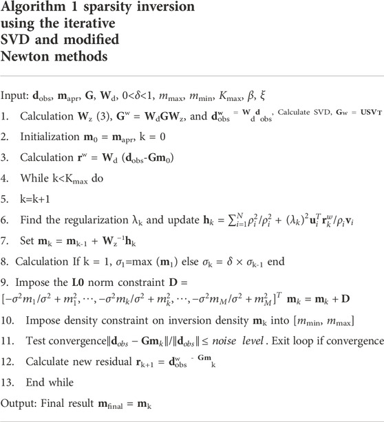
TABLE 1. Sparsity gravity inversion.

Inversion method using lanczos bidiagonalization compress algorithm

As the gravity data volume grows, the forward modeling matrix G becomes large. The large scale gravity data inversion increases its time and computer storage consumption and a strategy to handle such a massive amount of data is necessary Therefore, the inversion efficiency and the calculation storage should become a the focus of new investigations.

The minimization of the second part of Eq. 7 requires the calculation of the SVD of the forward modeling matrix, G^w. However, this process is not feasible for such large-scale matrices. For this reason, the Lanczos bidiagonalization compression algorithm, which project the gravity inversion problem onto a sub-space of small dimension, was adopted in this study. This algorithm allows one to solve large-scale and ill-posed gravity inversion problems efficiently.

By using the forward matrix, G^w, and the observed gravity data, d_obs, the Lanczos bidiagonalization compression scheme allows one to calculate the decomposition of B:

${{\mathbf{X}}^{\left(\mathrm{t}+1\right)}}^T{\mathbf{G}}^w{\mathbf{Y}}^t={\mathbf{B}}^t(17)$

where X^(t+1)∈R^(t+1)×N and Y^t∈R^t×M are orthonormal matrices, whereas B^t∈R^(t+1)×t is a lower bidiagonalization matrix. By using the Lanczos bidiagonalization process, a calculation based on t steps can be applied to the matrix G^w (Calvetti et al., 1999; 2000a; 2000b). Such computation process is presented in Appendix A. The bidiagonalization matrices B^t, X^t+1, and Y^t with orthonormal columns are generated such that:

$\begin{array}{cc}{\mathbf{G}}^w{\mathbf{Y}}^{\mathrm{t}}={\mathbf{X}}^{t+1}{\mathbf{B}}^t,& {\mathbf{X}}^{t+1}{e}^{t+1}\end{array}=\frac{{\mathbf{r}}^w}{{\Vert {\mathbf{r}}^w\Vert }_2}(18)$

where e^t+1∈R^(t+1)×1 represents a vector with a one in the first entry and 0 in the other entry. The columns of Y_t span the Krylov sub-space, κ_t, which can be expressed as:

${\kappa }_t\left({{\mathbf{G}}^w}^T{\mathbf{G}}^w,{{\mathbf{G}}^w}^T{\mathbf{r}}^w\right)=\mathrm{s}\mathrm{p}\mathrm{a}\mathrm{n}\left\{{{\mathbf{G}}^w}^T{\mathbf{r}}^w,\left({{\mathbf{G}}^w}^T{\mathbf{G}}^w\right){{\mathbf{G}}^w}^T{\mathbf{r}}^w,...,{\left({{\mathbf{G}}^w}^T{\mathbf{G}}^w\right)}^{t-1}{{\mathbf{G}}^w}^T{\mathbf{r}}^w\right\}(19)$

An approximate solution, h^t_(k), which lies in such Krylov sub-space has the form h^t_(k) = Y^tz^t_(k), z^t_(k)∈R^t×1 (Chung et al., 2008; Gazzola and Novati, 2013; Renaut et al., 2017). The second part of the original Eq. 7 becomes:

$P^{\alpha }\left({\mathbf{z}}_t\right)={\Vert {\mathbf{B}}_t{\mathbf{z}}_t-{\Vert {\mathbf{r}}^w\Vert }_2{\mathbf{e}}_{t+1}\Vert }_2^2+\alpha {\Vert {\mathbf{z}}_t\Vert }_2^2\to \min (20)$

where α is a new regularization factor for the new sub-space problem, which is determined via the W-GCV method. By comparing with full space forward matrix, G^w, with the new forward matrix, B^t, it appears that the latter one is smaller, t <<M. The projected space problem can be much more efficiency solved by using the SVD algorithm than the full space problem. The new inversion technique yields to a new update vector m_(k) = m_(k-1) + W_z⁻¹Y^tz_(k)^t. By comparing the forward matrix, G^w, of the full space and the matrix, B^t, of the projected space, one notices that the largest and lowest singular values of both matrixes are only an approximation (Golub et al., 1981). The flow of the new inversion method based on the Lanczos bidiagonalization compression algorithm is presented in Table 2. The choice of compression matrices t is determined by the characteristic of gravity forward matrix G^w.

TABLE 2

TABLE 2. Sparsity gravity inversion based on the Lanczos bidiagonalization compression algorithm.

In the gravity inversion, the forward matrix, G^w, and its inverse consume al a large amount of computational memory and time when compared to other matrices. By analyzing thee compression of the G^w matrix it appears that the memory storage is required only for the Ο(M) during the inversion calculation. By considering the difference in the computational power needed for the original G^w matrix and the compress matrix B^t, it appears that the SVD method plays the most important role. The computation of the full algorithm requires the SVD for a matrix of size N × M, the generation of the update h_k, via the SVD, and then the estimate of the regularization parameter, via the W-GCV algorithm. By applying the SVD method in the inversion, the memory consumption used during the regularization parameter calculation is negligible in the large scale inversion problem when compared to the other calculations. In a large scale inversion problem (N << M) the largest amount of computational power is required by the calculation of the Ο(M²N) terms to define the SVD (Van Loan and Golub, 1996; Line 5 of table, p. 254). However, after the Lanczos bidiagonalization of the original forward matrix, G^w, is achieved, the SVD step for B_t is mostly dominated by the calculation of the Ο(t³) terms. Moreover, the update vector z_k^t is a matrix vector, which multiplies the Ο(Nt) matrix and generates the Ο(MNt) term (Paige and Saunders, 1982). Due to the condition t << M, the calculation of the Ο(MNt) element is actually Ο(MN) with a scale number t, and this method has been proven to be more efficient when compared to the calculation of Ο(M²N). Based on these results, we the forward matrix compression improves the inversion calculated efficiency and reduces the computational power and memory storage.

Choice of the regularization parameter

The regulation parameter affects the accuracy of the solution. Moreover, it is a very important for the studies in the inversion research field (Engl et al., 1996). The GCV algorithm is a classical algorithm, which is used to define a regularization parameter. However, many studies show that the regularization parameters determined via this method are occasionally to small and the solutions are under-smooth in several practical applications (Friedman and Silverman, 1989; Cummins et al., 2001; Vogel, 2002; Kim and Gu, 2004; Vio et al., 2004). To overcome this disadvantage, a weighted parameter was introduced to modify the GCV algorithm (W-GCV), which it has been shown to predict the missing values of the data fairly well. Moreover, it is a predictive statistics-based method that does not require a priori estimates of the error norm. The advantages of the W-GCV method have been investigated in many domains (Golub and Wahba, 1979; Golub and Von Matt, 1997; Hansen, 2005; Chung et al., 2008; Gholami and Siahkoohi, 2010; Meng et al., 2016). Here, each data point value, r^w, is—in turn–removed from the calculation to find the a value, which minimizes the prediction errors. The expression of such W-GCV function is the following:

$WGC{V}_{{\mathbf{G}}^w,{\mathbf{r}}^w}\left(\lambda \right)=\frac{\mathrm{N}{\Vert \left(\mathbf{I}-{\mathbf{G}}^w{{\mathbf{G}}^w}_{\lambda }^{*}\right){\mathbf{d}}^w\Vert }_2^2}{{\left(trace\left(\mathbf{I}-\omega {\mathbf{G}}^w{{\mathbf{G}}^w}_{\lambda }^{*}\right)\right)}^2}(21)$

where ${{\mathbf{G}}^w}_{\lambda }^{*}={\left(G^{wT}{G}^w+{\lambda }^{2}I\right)}^{-1}{G^w}^T$. In this way, an optimal regularization factor, λ, is obtained. Upon the application of the SVD, Eq. 9 is transformed into:

$WGC{V}_{{\mathbf{G}}^w,{\mathbf{r}}^w}\left(\lambda \right)=\frac{\mathrm{N}\left({\displaystyle \sum }_{i=1}^N{\left(\frac{{\lambda }^2{\mathbf{u}}_i^T{\mathbf{r}}^w}{{\rho }_i^2+{\lambda }^2}\right)}^2+{\displaystyle \sum }_{i=N+1}^M{\left({\mathbf{u}}_i^T{\mathbf{r}}^w\right)}^2\right)}{\left(\left(M-N\right)+{\displaystyle \sum }_{i=1}^N\frac{\left(1-\omega \right){\rho }_i^2+{\lambda }^2}{{\rho }_i^2+{\lambda }^2}\right)}(22)$

This is a computationally convenient technique to evaluate the W-CGV function, which can be easily applied to standard minimization algorithms. It must be noticed that the function depends now on a new parameter, ω, which appears in the denominator trace term. The choice of ω is necessary for the regularization parameter. The smoothest solution is obtained when ω < 1, whereas a less smooth solution can be obtained when ω > 1. Therefore, the choice of ω is pivotal for the inversion. In several applications, the value of ω is determined by experience (Kim and Gu, 2010). To increase its practical application, an adaptive approach for the determination of ω was investigated and it is discussed in Appendix A.

Here, the W-GCV of the Tikhonov regularization on the full system of gravity inversion is discussed. The projected subspace, B_t, can be obtained by using the Lanczos bidiagonalization compression algorithm. In this case, the expression of the projected subspace W-GCV can be expressed as:

$\begin{array}{l}WGC{V}_{B_t,{\Vert {\mathbf{r}}^w\Vert }_2{\mathbf{e}}^{t+1}}\left(\omega ,\lambda \right)=\frac{t{\Vert \left(I-B_t{B}_t^{*}\right){\Vert {\mathbf{r}}^w\Vert }_2{\mathbf{e}}^{t+1}\Vert }_2^2}{{\left(trace\left(I-\omega B_t{B}_t^{*}\right)\right)}^2}\\ =\frac{t{\left({\Vert {\mathbf{r}}^w\Vert }_2\right)}^2\left({{\displaystyle \sum }_{i=1}^t{\left(\frac{{\alpha }^2}{{\delta }_i^2+{\alpha }^2}{\left[P_t^T{e}^{t+1}\right]}_i\right)}^2+\left({\left[P_t^T{e}^{t+1}\right]}_{t+1}\right)}^2\right)}{{\left(1+{\displaystyle \sum }_{i=1}^t\frac{\left(1-\omega \right){\delta }_i^2+{\alpha }^2}{{\delta }_i^2+{\alpha }^2}\right)}^2}\end{array}(23)$

where, P_t is an orthogonal matrix calculated via the SVD of sparse B_t and δ represents a singular value of B_t.

${\mathbf{B}}_k={\mathbf{P}}_k\left[\begin{array}{c}{\mathbf{\Delta }}_k\\ {\mathbf{0}}^T\end{array}\right]{\mathbf{Q}}_k^T(24)$

An optimal regularization parameter α can be used in a fixed projected problem of size t such that the resulting solution appropriately regularizes the full problem. This means that α_opt ≈ λ_opt, where α_opt and λ_opt are the optimal regularization parameters for the projected and full problems, respectively.

Adaptive lanczos bidiagonalization compression algorithm

To calculate the memory requirements for large scale data, the Lanczos bidiagonalization compression algorithm can be applied. In this case, the compression rate, t, is very important for the calculated efficiency and the accuracy of the inversion. A large value of t does not improve the calculated efficiency of the gravity inversion, contrarily to a small value of t. In several studies, the value of t is determined by experience. However, this method cannot be applied in the practical gravity data applications. Defining a method to calculate t according to the inversion parameters is then very important. Therefore, an adaptive Lanczos bidiagonalization compression algorithm is used in this study. The W-GCV algorithm is also applied to determine the compression factor t. By using Eq. 23, t is regard as a solver parameter and Eq. 23 becomes:

$\begin{array}{l}{W}_{B_t}\left(t\right)=\frac{t{\Vert \left(I-B_t{B}_t^{*}\right){\Vert {\mathbf{r}}^w\Vert }_2{\mathbf{e}}^{t+1}\Vert }_2^2}{{\left(trace\left(I-\omega B_t{B}_t^{*}\right)\right)}^2}\\ =\frac{t{\left({\Vert {\mathbf{r}}^w\Vert }_2\right)}^2\left({{\displaystyle \sum }_{i=1}^t{\left(\frac{{\alpha }^2}{{\delta }_i^2+{\alpha }^2}{\left[P_t^T{e}^{t+1}\right]}_i\right)}^2+\left({\left[P_t^T{e}^{t+1}\right]}_{t+1}\right)}^2\right)}{{\left(1+{\displaystyle \sum }_{i=1}^t\frac{\left(1-\omega \right){\delta }_i^2+{\alpha }^2}{{\delta }_i^2+{\alpha }^2}\right)}^2}\end{array}(25)$

In this case W_Bt(t) is used to determine the compression factor t in the implementation. Moreover, its value converges. Therefore, the iteration process terminates when the value change are very small:

$\left|\frac{W_{B_t}\left(t+1\right)-W_{B_t}\left(t+1\right)}{W_{B_t}\left(1\right)}\right|<tol(26)$

where, tol is a chosen value for the tolerance. The compression factor t can be then selected effectively and automatically.

Synthetic examples

A complex synthetic example is used to analyze the advantages of the inversion method proposed in this paper. The goals of this test are three: 1) estimate the accuracy of sparsity gravity inversion results, which are solved by combining the regularization SVD algorithm and the modified Newton algorithm. Due to the comparison between the sparsity inversion and smooth inversion results, an approximate inversion method can be obtained; 2) compare the influences of different values of ω by using different regularization parameters; and 3) estimate the accuracy of the inversion method via the Lanczos bidiagonalization method and compare it to the full sparsity gravity inversion technique. By using this synthetic example, the accuracy and the efficiency of the inversion can be easily estimated. The whole calculation was performed on a desktop computer with Intel Core i7-7700 HQ and 8.00 GB RAM.

Figure 1B) shows the gravity data calculated for different anomalous bodies (in Figure 1A)). Detailed information about the anomalous bodies can be found in Table 3. The research region was distributed over a 4,000 × 4,000 m² area with sample spacing of 100 m. A total of 40 × 40 = 1,600 observed gravity data points were used during the inversion and 3% of noise has been added in the gravity data. The depth was 2000 m. According to this information, 40 × 40 × 20 = 32,000 discrete prisms of 100 m size can be defined. A resulting kernel matrix, G, of size 1,600 × 32000 was applied to the full space data inversion. Via the Lanczos bidiagonalization compression algorithm the sub-space inversion was obtained. In the whole inversion, the depth weighting factor β = 1 was use. The descending factor δ = 0.9 was instead selected to ensure that the sparsity parameter would decrease during the inversion iterations and to ensure that the global optimum solution would be obtained. The corresponding upper and lower density contrast density threshold are m_max = 1.0 g/cm³ and m_min = 0.0 g/cm³. The inversion iterations terminates when the error of the data is smaller than the noise level or the maximum number of iterations is reached. The observed gravity data error is a key point for the evaluation of inversion results.

FIGURE 1

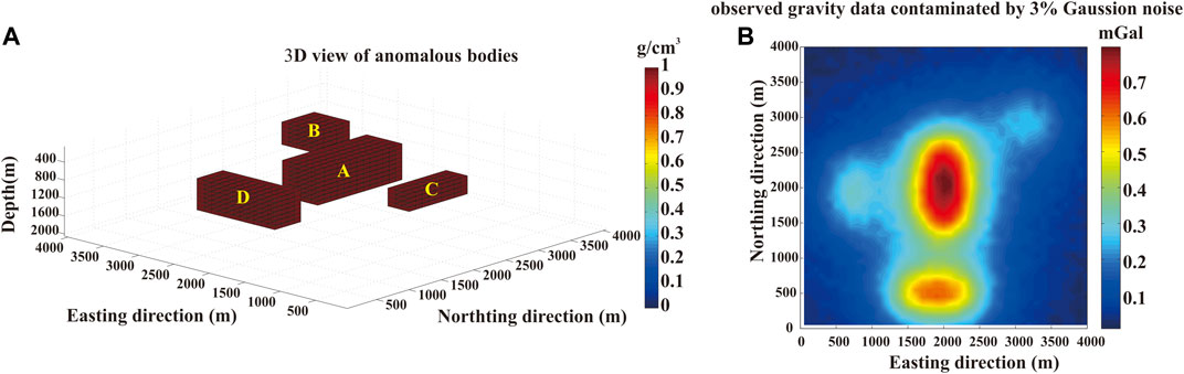
FIGURE 1. (A) 3D view of the anomalous body density distributions; (B) observed gravity data contaminated by noise within the 3% of the maximum value of the gravity data.

TABLE 3

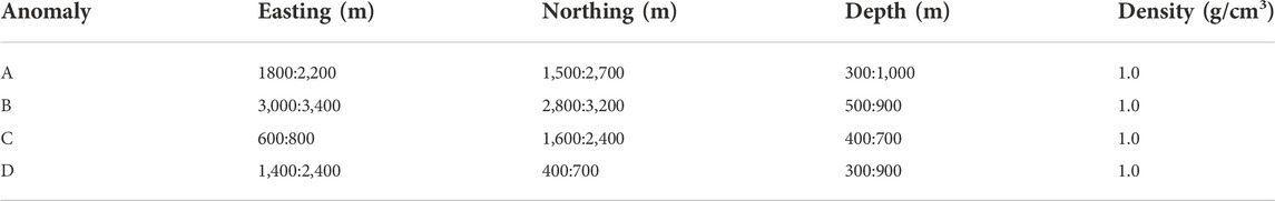
TABLE 3. Parameters of the sub-surface anomalous bodies.

In the simulation test, the density value and the distribution of the anomalous bodies were known. Therefore, the model error was used to evaluate the accuracy of the inversion results. The relative error of the reconstructed model is expressed by:

$Er{r}_{model}=\frac{{\Vert {\mathbf{m}}_0-{\mathbf{m}}_{\mathit{final}}\Vert }_2}{{\Vert {\mathbf{m}}_0\Vert }_2}(27)$

where m₀ is the true value of the simulation model density and m_final is the final inversion result.

Here, a comparison between the inversion results obtained via the classical smooth inversion method and the sparsity inversion method (Figure 2 and Figure 3, respectively) shows the advantages of the latter one proposed in this paper. The trend of the data misfit ($\frac{\parallel d_{obs}-{Gm}_k\parallel }{\parallel d_{obs}\parallel }$), the model misfit (Err), and the regularization parameters of the results of the two inversion methods are shown in Figure 4.

FIGURE 2

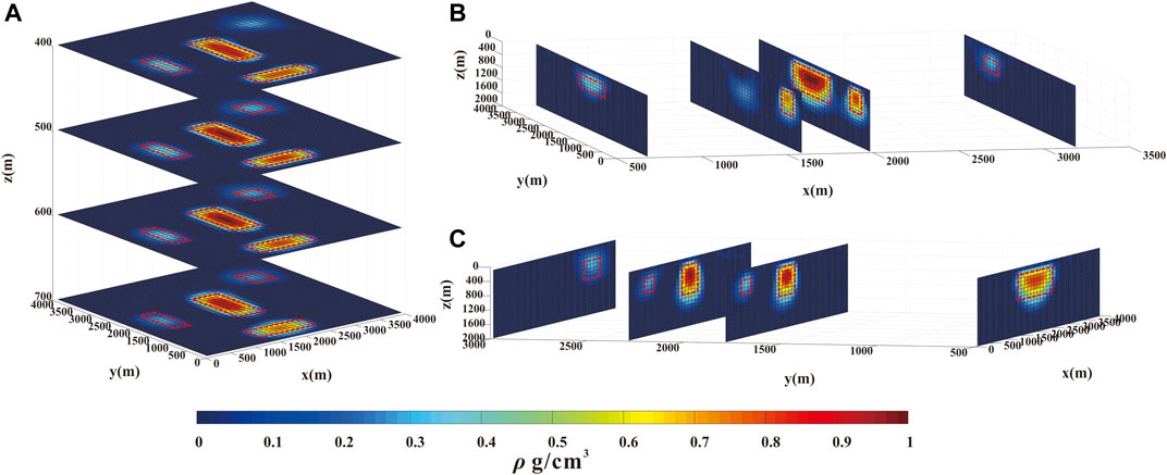
FIGURE 2. (A) the plan section of the recovered density model obtained by the inversion of the gravity anomaly at z = -400 m, -500 m, -600 m, and -700 m (B) X-direction section of the recovered density model at x = 700 m, 1,600 m, 2000 m and 3,200 m. (C) Y-direction section of the recovered density model at y = 500 m, 1800 m, 2,300 m, and 3,000 m.

FIGURE 3

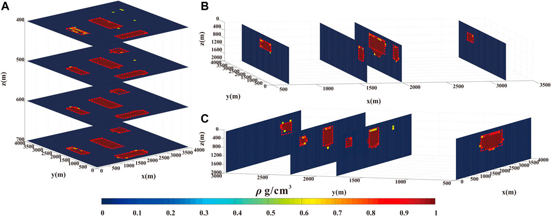
FIGURE 3. (A) the plan section of the recovered density model obtained via the inversion of the gravity anomaly at z = -400 m, -500 m, -600 m, and -700 m (B) X-direction section of the recovered density model at x = 700 m, 1,600 m, 2000 m, and 3,200 m. (C) Y-direction section of the recovered density model at y = 500 m, 1800 m, 2,300 m, and 3,000 m.

FIGURE 4

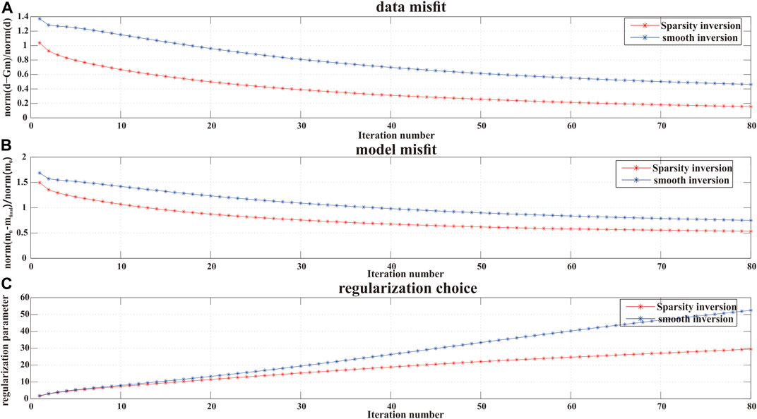
FIGURE 4. Comparison between the sparsity inversion and the smooth inversion. (A) Progression of the data misfit: sparsity inversion in red -* and smooth inversion in blue -*; (B) Model misfit; (C) Regularization choice of each iteration.

The pink dotted lines shown in Figures 2, 3 show the positions of the true distribution of the anomalous bodies. The different depth slices and the horizontal slices of inversion results are shown for the sake of clarity. Initially, the inversion density contrasts are both equal to zero. By the analysis of the depth of the slices, the horizontal distribution of the anomalous bodies can be easily estimated. The results of the classical smooth inversion are shown in Figure 2A): the inversion density distribution is larger than the true model. Moreover, the density boundary is blurred and the density value is smaller than the true value. The vertical slices of the smooth inversion results are reported in Figure 2B,C. The inversion results show some leakage of the anomalous bodies. The smooth inversion method provides a relatively accurate inversion result despite the densities of the inversion small bodies are much lower than true density. The sparsity inversion results are shown in Figure 3. Due to the principle of the sparsity inversion method, the block inversion results can be obtained, and they are close to the true anomalous bodies. The blocker results can be obtained via the sparsity inversion technique and they are more precise, as shown in Figure 4. Experimental methods need a comprehensive theory for a deep and quantitative understanding of the results. The data misfit and the model misfit are used to show the accuracy of the inversion results. The differences between the observed gravity data and the calculated gravity data are shown in Figure 4A. In the inversion, initially the data misfit function is large and then, it decays quickly during the inversion iterations. As the inversion results become close to the true solution, the value of the data misfit function decreases. Figure 4A shows that the convergence degree of the sparsity gravity inversion provides a higher performance than the smooth inversion. The difference between the inversion density value distribution and the true density value distribution is shown in Figure 4B. The model misfit is only applied in the case of the synthetic test: the accuracy of the inversion results by using different inversion method has been tested and in this simulation, the sparsity inversion results are more similar to true values when compared to the smooth inversion results. Figure 4C shows the change in the regularization parameters during the inversion process.

In this section the influence on the inversion results upon using the W-GCV method with different values of ω is analyzed. The sparsity inversion technique is applied to show the advantage of the W-GCV algorithm. Figure 5 shows the data convergence of the sparsity inversion method by using the both W-GCV with different ω and the GCV algorithm. The best inversion results are obtained with the W-GCV algorithm. Moreover, the influence of regularization parameters on the results could be easily captured by this comparison: the choice of a suitable value of ω is fundamental, as well as the adaptive W-GCV method.

FIGURE 5

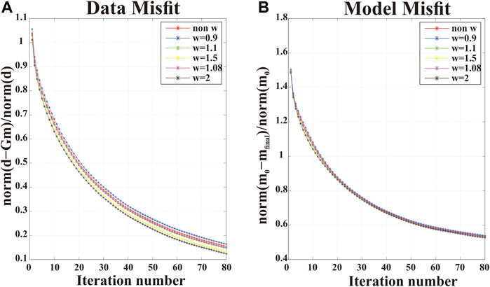
FIGURE 5. Curve of the data and model misfit with different values of ω. (A) The plot shows that the different values of ω have an impact on the inversion data convergence and (B) on the accuracy of the inversion.

To show the compression effect, the inversion results obtained by using the algorithm one described in Table 1 and the algorithm 2 described in Table 2 are compared. The corresponding inversion results are shown in Figure 6. The compress factor, which has a value between 30 and 11, is shown in Figure 7. The small dimension of the new replaced matrix reduces the inversion time and the computational power required to perform the calculation. The comparison between Figures 4, 6 shows that the compress algorithm does not affect the inversion accuracy. Both algorithms are able to recover the accurate density distribution of the sub-surface, as shown in Figure 8. Moreover, both the data misfit and the model misfit are consistent. Therefore, the sparsity gravity inversion based on the Lanczos bidiagonalization compress algorithm not only provides an accurate inversion result, but also increases the inversion efficiency. Moreover, the adaptive compress algorithm achieves an optimal value for the compression factor, t.

FIGURE 6

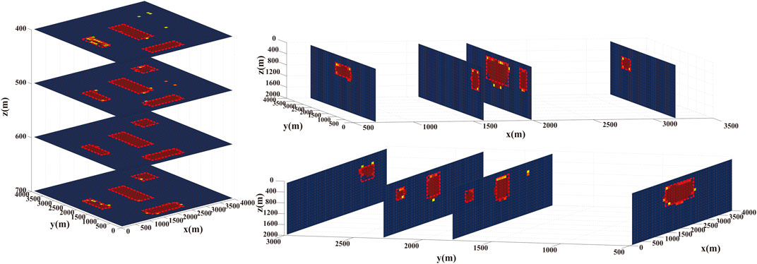
FIGURE 6. Similarly to Figures 2, 3 but in this case the inversion results were obtained by using the sparsity inversion method based on the Lanczos bidiagonalization compression algorithm.

FIGURE 7

FIGURE 7. Choice of the compress factor for each iteration number using the adaptive Lanczos bidiagonalization method.

FIGURE 8

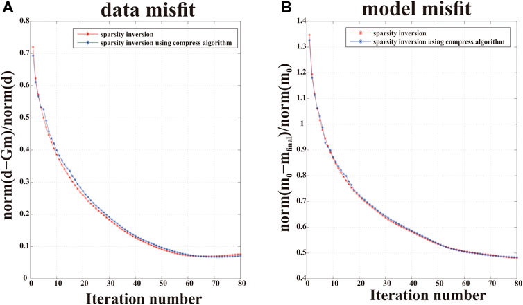
FIGURE 8. Comparison between the sparsity inversion and the sparsity inversion based on the Lanczos bidiagonalization compress algorithm; (A)trend of the data misfit; (B) model misfit generated by the difference between the two methods.

Real data application

To show the practical implications of the inversion method proposed in this paper, a well-known Mobrun ore body research, situated in the North-East of Noranda, Quebec was used. The residual gravity data is shown in Figure 9. The anomaly pattern can be associated to a massive body consisting of a base metal sulphide (mainly pyrite) embedded in volcanic rocks of the middle Precambrian age (Grant and West, 1965). The original gravity pattern of the sample is shown in Figure 10.1 in the paper of Grant and West (1965). In the current application, the data was carefully digitized and input into a regular grid of 30 × 30 = 900 data points, which are spaced 20 m × 20 m over the East and North directions, respectively. Moreover, the average density of the core samples of the ore bodies measured 4.6 g/cm³ whereas the density of the host rocks was 2.7 g/cm³. Thus, the density contrast of the sulfide ore body measured 1.9 g/cm³ (Grant and West, 1965). To apply the inversion method presented in this manuscript into this aforementioned region, the sub-surface space was discretized into 30 × 30 × 15 = 13,500 cells along the East, North, and depth directions, respectively. The side of each cell measures 20 m. The noise distribution used in this application was σ_i = (0.03 (g_obs)_i + 0.004|| g_obs ||₂). The density contrast constraint of the sulfide ore body has a value between 0 g/cm³ and 1.9 g/cm³.

FIGURE 9

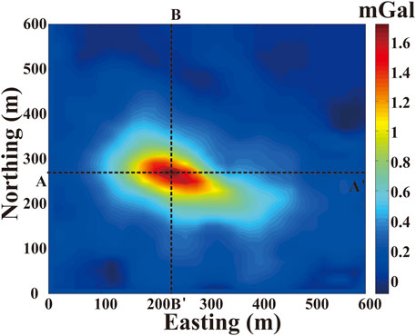
FIGURE 9. Residual bouguer anomaly map of the Mobrun ore body, northeast of Noranda, Quebec.

The distribution of the ore body was obtained by applying the method discussed in this paper. The different depth slices (at z = -20 m, z = -100, and z = -180) of the ore body density distribution are shown in Figure 10. From this figure, the strike of the sulfide body can be clearly observed and it elongates from NW to SE. Two vertical slices (A-A′ at north direction = 260 m and B-B’ east direction = 240 m) are present and illustrated in Figure 11, which shows the vertical distributions of the recovered density body. The 3D view of the ore body density distribution, which was obtained by considering a density cut off 0.8 g/cm³, is shown in Figure 12.

FIGURE 10

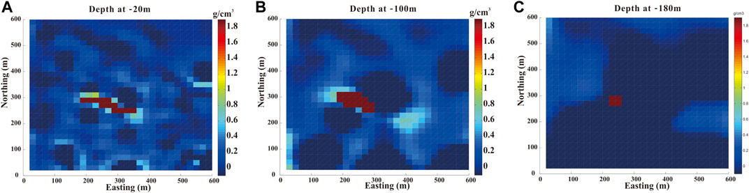
FIGURE 10. Depth slice measured at z = -20 m via the recovered density distribution obtained by using the inversion method proposed in this paper (A); Depth slice at z = -100 m (B); Depth slice at z = -180 m (C).

FIGURE 11

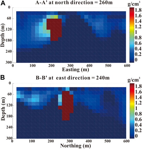
FIGURE 11. Cross sections along the North direction = 260 m (A) and along the East direction = 240 m (B) of the inversion density distribution obtained by using the inversion method discussed in this paper.

FIGURE 12

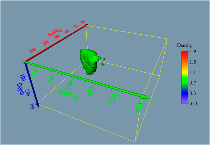
FIGURE 12. 3D view of the inversion density of the Mobrun ore body for a cut off density of 0.8 g/cm³.

According to density distribution of the inversion results, the top and bottom depth of the ore body measure about 20 and 180 m, respectively. The inversion results effectively show the position of the ore body in this region. The true information of the sulfide body and the mineralized zone can be obtained by using the information available for several boreholes. According to the drilling data presented in Figure 13, the density distribution and the value of the ore body measures about 17 m and it extends to 187 m (Figure 13) (Grant and West 1965). Therefore, the inversion results obtained by using the inversion method proposed in this paper agree with the results available from the drilling experiments and the data obtained by Aghajani et al. (2009).

FIGURE 13

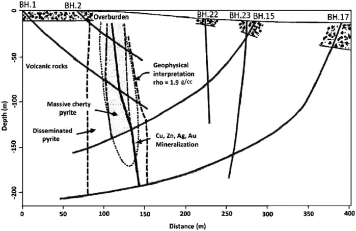
FIGURE 13. Drilling information and geological section of the Mobrun sulfide body with its geophysical interpretation (Grant and West 1965).

Conclusion

A new fast sparsity inversion method based on the regularization of the SVD algorithm is examined in this paper. The addition of the approximate L0 norm improves the sparseness of the inversion model characteristics. A W-GCV method is applied to choose a suitable regularization parameter. In the W-GCV method, the parameter ω, which is determined via an adaptive and automatic algorithm, is used. To solve the inversion efficiency of the large-scale gravity data, a Lanczos bidiagonalization compression algorithm is introduced to reduce the dimension of the original gravity forward matrix. Moreover, to obtain an optimal compression factor, an adaptive choice method was investigated. By using the inversion method proposed in this paper, not only a sparsity inversion with a block density distribution can be obtained, but also the inversion efficiency can be improved. Synthetic data contaminated by noise was used to test such inversion method. The inversion results obtained via the full space sparsity and the project sub-space inversion methods using a compression algorithm produce very similar results. In this way, the sub-surface density distribution of the anomalous bodies could be obtained precisely. Finally, a real gravity data set from the Mobrun sulfide body was used to test the ability of the method in a real-world application. The inversion results are in good agreement with the data provided by the drilling information and the geological data. This new inversion method shows to have a huge potential in the data inversion field.

Data availability statement

The original contributions presented in the study are included in the article/supplementary material, further inquiries can be directed to the corresponding author.

Author contributions

MZ and WY contributed to the application of methods and manucsript preparation. LJ, LF and ZZ contributed to the article writing and to its scientific development.

Funding

In part by the Research on Detection and Positioning Technology of Underground Concealed Military Engineering Based on Gravity under Grant 6142414200815.

Conflict of interest

The authors declare that the research was conducted in the absence of any commercial or financial relationships that could be construed as a potential conflict of interest.

Publisher’s note

All claims expressed in this article are solely those of the authors and do not necessarily represent those of their affiliated organizations, or those of the publisher, the editors and the reviewers. Any product that may be evaluated in this article, or claim that may be made by its manufacturer, is not guaranteed or endorsed by the publisher.

References

Abedi, M., Gholami, A., Norouzi, G. H., and Fathianpour, N. (2013). Fast inversion of magnetic data using lanczos bidiagonalization method. J. Appl. Geophys. 90 (90), 126–137. doi:10.1016/j.jappgeo.2013.01.008

CrossRef Full Text | Google Scholar

Aghajani, H., Moradzadeh, A., and Zeng, H. (2009). Normalized full gradient of gravity anomaly method and its application to the Mobrun sulfide body, Canada. World Appl. Sci. J. 6 (3), 393–400.

Google Scholar

Bertete-Aguirre, H., Cherkaev, E., and Oristaglio, M. (2002). Non-smooth gravity problem with total variation penalization functional. Geophysical Journal International 149 (2), 499–507.

CrossRef Full Text | Google Scholar

Blakely, R. J. (1996). Potential theory in gravity and magnetic applications. Cambridge University Press.Chennai

Google Scholar

Boulanger, O., and Chouteau, M. (2001). Constraints in 3D gravity inversion. Geophys. Prospect. 49 (2), 265–280. doi:10.1046/j.1365-2478.2001.00254.x

CrossRef Full Text | Google Scholar

Calvetti, D., Golub, G. H., and Reichel, L. (1999). Estimation of the L-curve via Lanczos bidiagonalization. BIT Numerical Mathematics 39 (4), 603–619.

CrossRef Full Text | Google Scholar

Camacho, A. G., Fernández, J., González, P. J., Rundle, J. B., Prieto, J. F., and Arjona, A. (2009). Structural results for La Palma island using 3-D gravity inversion. J. Geophys. Res. 114 (B5), B05411. doi:10.1029/2008jb005628

CrossRef Full Text | Google Scholar

Cella, F., and Fedi, M. (2012). Inversion of potential field data using the structural index as weighting function rate decay. Geophysical Prospecting 60 (2), 313–336

CrossRef Full Text | Google Scholar

Chan, R. H., Ho, C. W., Leung, C. Y., and Nikolova, M. (September 2005). Minimization of detail-preserving regularization functional by Newton's method with continuation. Proceedings of the IEEE Int. Conf. Image.Genova, Italy, doi:10.1109/ICIP.2005.1529703

CrossRef Full Text | Google Scholar

Chasseriau, P., and Chouteau, M. (2003). 3D gravity inversion using a model of parameter covariance. J. Appl. Geophys. 52 (1), 59–74. doi:10.1016/s0926-9851(02)00240-9

CrossRef Full Text | Google Scholar

Chung, J., Nagy, J., and O’Leary, D. P. (2008). A weighted GCV method for Lanczos hybrid regularization. Electron. Trans. Numer. Analysis 28, 149–167.

Google Scholar

Commer, M. (2011). Three-dimensional gravity modelling and focusing inversion using rectangular meshes. Geophys. Prospect. 59 (5), 966–979. doi:10.1111/j.1365-2478.2011.00969.x

CrossRef Full Text | Google Scholar

Cummins, D. J., Filloon, T. G., and Nychka, D. (2001). Confidence intervals for nonparametric curve estimates: Toward more uniform pointwise coverage. J. Am. Stat. Assoc. 96, 233–246. doi:10.1198/016214501750332811

CrossRef Full Text | Google Scholar

Engl, H. W., Hanke, M., and Neubauer, A. (1996). Regularization of inverse problems, 375. Springer Science & Business Media.

CrossRef Full Text | Google Scholar

Farquharson, C. G., and Silverman, B. W. (2008). Constructing piecewise-constant models in multidimensional minimum-structure inversions. Geophysics 73 (1), K1–K9

CrossRef Full Text | Google Scholar

Friedman, J. H., and Silverman, B. W. (1989). [Flexible parsimonious smoothing and additive modeling]: Response. Technometrics 31 (1), 35–21. doi:10.2307/1270362

CrossRef Full Text | Google Scholar

Gazzola, S., and Novati, P. (2013). Multi-parameter Arnoldi-Tikhonov methods. Electron. Trans. Numer. Anal. 40, 452–475.

Google Scholar

Gholami, A., and Siahkoohi, H. R. (2010). Regularization of linear and non-linear geophysical ill-posed problems with joint sparsity constraints. Geophys. J. Int. 180 (2), 871–882. doi:10.1111/j.1365-246x.2009.04453.x

CrossRef Full Text | Google Scholar

Golub, G. H., Luk, F. T., and Overton, M. L. (1981). A block Lanczos method for computing the singular values and corresponding singular vectors of a matrix. ACM Trans. Math. Softw. 7, 149–169. doi:10.1145/355945.355946

CrossRef Full Text | Google Scholar

Golub, G. H., and Von Matt, U. (1997). Generalized cross-validation for large-scale problems. J. Comput. Graph. Statistics 6 (1), 1–34. doi:10.2307/1390722

CrossRef Full Text | Google Scholar

Golub, G. H., and Wahba, H. G. (1979). Generalized cross-validation as a method for choosing a good ridge parameter. Technometrics 21 (2), 215–223. doi:10.1080/00401706.1979.10489751

CrossRef Full Text | Google Scholar

Grant, F. S., and West, G. F. (1965). Interpretation theory in applied geophysics. New York: McGraw-Hill.

Google Scholar

Hansen, P. C. (2005). Rank-deficient and discrete ill-posed problems: numerical aspects of linear inversion, 4. Siam.

Google Scholar

Kahoo, A. R., Kalateh, A. N., and Salajegheh, F. (2015). Interpretation of gravity data using 2-D continuous wavelet transformation and 3-D inverse modeling. J. Appl. Geophys. 121, 54–62. doi:10.1016/j.jappgeo.2015.07.008

CrossRef Full Text | Google Scholar

Kim, Y. J., and Gu, C. (2004). Smoothing spline Gaussian regression: More scalable computation via efficient approximation. J. R. Stat. Soc. B, 337–356. doi:10.1046/j.1369-7412.2003.05316.x

CrossRef Full Text | Google Scholar

Kim, Y. J., and Gu, C. (2010). Smoothing spline Gaussian regression: More scalable computation via efficient approximation. J. R. Stat. Soc. B 66 (2), 337–356. doi:10.1046/j.1369-7412.2003.05316.x

CrossRef Full Text | Google Scholar

Last, B. J., and Kubik, K. (1983). Compact gravity inversion. Geophysics 48 (6), 713–721.

CrossRef Full Text | Google Scholar

Li, Y., and Oldenburg, D. W. (1998). 3-D inversion of gravity data. Geophysics 63 (1), 109–119. doi:10.1190/1.1444302

CrossRef Full Text | Google Scholar

Li, Y., and Oldenburg, D. W. (2003). Fast inversion of large-scale magnetic data using wavelet transforms and a logarithmic barrier method. Geophysical Journal International 152 (2), 251–265.

CrossRef Full Text | Google Scholar

Loke, M. H., Acworth, I., and Dahlin, T. (2003). A comparison of smooth and blocky inversion methods in 2D electrical imaging surveys. Exploration Geophysics 34 (3), 182–187.

CrossRef Full Text | Google Scholar

Meng, Z. (2015). “3 D gravity inversion based on sparse recovery,” in International workshop and gravity, electrical & magnetic methods and their applications (China: Chenghu), 19–22.

CrossRef Full Text | Google Scholar

Meng, Z. (2016). 3D inversion of full gravity gradient tensor data using SL0 sparse recovery. J. Appl. Geophys. 127, 112–128. doi:10.1016/j.jappgeo.2016.02.010

CrossRef Full Text | Google Scholar

Meng, Z., Li, F., Zhang, D., Xu, X., and Huang, D. (2016). Fast 3D inversion of airborne gravity-gradiometry data using Lanczos bidiagonalization method. J. Appl. Geophys. 132, 211–228. doi:10.1016/j.jappgeo.2016.07.013

CrossRef Full Text | Google Scholar

Meng, Z. (2018). Three-dimensional potential field data inversion with L0 quasinorm sparse constraints. Geophys. Prospect. 66 (3), 626–646. doi:10.1111/1365-2478.12591

CrossRef Full Text | Google Scholar

Mohimani, H., Babaie-Zadeh, M., and Jutten, C. (2009). A fast approach for overcomplete sparse decomposition based on smoothed $\ell ^{0}$ norm. IEEE Trans. Signal Process. 57 (1), 289–301. doi:10.1109/tsp.2008.2007606

CrossRef Full Text | Google Scholar

Nocedal, J., and Wright, S. J. (2006). Numerical optimization 2nd edition.

Google Scholar

Oldenburg, D. W., and Pratt, D. A. (2007). Geophysical inversion for mineral exploration: A decade of progress in theory and practice. Proc. Explor. 7 (5), 61–95.

Google Scholar

Paige, C. C., and Saunders, M. A. (1982). LSQR: An algorithm for sparse linear equations and sparse least squares. ACM Transactions on Mathematical Software (TOMS) 8 (1), 43–71.

CrossRef Full Text | Google Scholar

Pilkington, M. (2008). 3D magnetic data-space inversion with sparseness constraints. Geophysics 74 (1), L7–L15. doi:10.1190/1.3026538

CrossRef Full Text | Google Scholar

Pilkington, M. (2009). 3D magnetic data-space inversion with sparseness constraints. Geophysics 74 (1), L7–L15.

CrossRef Full Text | Google Scholar

Rezaie, M., Moradzadeh, A., and Nejati Kalate, A. (2017). 3D gravity data-space inversion with sparseness and bound constraints. J. Min. Environ. 8 (2), 227–235.

Google Scholar

Shamsipour, P., Chouteau, M., and Marcotte, D. (2011). 3D stochastic inversion of magnetic data. J. Appl. Geophys. 73 (4), 336–347. doi:10.1016/j.jappgeo.2011.02.005

CrossRef Full Text | Google Scholar

Silva, J. B., and Barbosa, V. C. (2006). Interactive gravity inversion interactive gravity inversion. Geophysics 71 (1), J1–J9.

CrossRef Full Text | Google Scholar

Toushmalani, R., and Saibi, H. (2015). Fast 3D inversion of gravity data using Lanczos bidiagonalization method. Arabian J. Geosciences 8 (7), 4969–4981.doi:10.1007/s12517-014-1534-4

CrossRef Full Text | Google Scholar

Uieda, L., and Barbosa, Valéria C. F. (2017). Fast nonlinear gravity inversion in spherical coordinates with application to the south American moho. Geophys. J. Int. 208 (1), 162–176. doi:10.1093/gji/ggw390

CrossRef Full Text | Google Scholar

Van Loan, C. F., and Golub, G. (1996). Matrix computations (Johns Hopkins studies in mathematical sciences). Matrix Computations

Google Scholar

Vatankhah, S., Anne Renaut, R., and Ardestani, V. E. (2018). A fast algorithm for regularized focused 3D inversion of gravity data using randomized singular-value decomposition. Geophysics 83 (4), G25–G34. doi:10.1190/geo2017-0386.1

CrossRef Full Text | Google Scholar

Vatankhah, S., Ardestani, V. E., Niri, S. S., Renaut, R. A., and Kabirzadeh, H. (2019). Igug: A matlab package for 3D inversion of gravity data using graph theory. Comput. Geosciences 128, 19–29. doi:10.1016/j.cageo.2019.03.008

CrossRef Full Text | Google Scholar

Vatankhah, S., Renaut, R. A., and Ardestani, V. E. (2017). 3-D Projected L 1 inversion of gravity data using truncated unbiased predictive risk estimator for regularization parameter estimation. Geophys. J. Int. 210 (3), 1872–1887. doi:10.1093/gji/ggx274

CrossRef Full Text | Google Scholar

Vio, R., Ma, P., Zhong, W., Nagy, J., Tenorio, L., and Wamsteker, W. (2004). Estimation of regularization parameters in multiple-image deblurring. Astron. Astrophys. 423 (3), 1179–1186. doi:10.1051/0004-6361:20047113

CrossRef Full Text | Google Scholar

Vogel, C. R. (2002). Computational methods for inverse problems, 23. Siam.

Voronin, S., Mikesell, D., and Nolet, G. (2015). Compression approaches for the regularized solutions of linear systems from large-scale inverse problems. GEM-International J. Geomathematics, 6(2), Wang, Y., Liu, P., Li, Z., et al. (2013). Data regularization using Gaussian beams decomposition and sparse norms. J. Inverse Ill-Posed Problems, 21(1), 1–23, doi:10.1515/jip-2012-0030

CrossRef Full Text | Google Scholar

Wang, Y., Liu, P., Li, Z., Sun, T., Yang, C., and Zheng, Q. (2013). Data regularization using Gaussian beams decomposition and sparse norms. Journal of Inverse and Ill-Posed Problems 21 (1), 1–23.

CrossRef Full Text | Google Scholar

Zhdanov, M. S. (2002). Geophysical inverse theory and regularization problems 36. Elsevier

Appendix A: Lanczos bidiagonalization compression algorithm

The Lanczos bidiagonalization compression algorithm is based on the full space forward matrix, G^w, and on its corresponding observed data, d^w. The calculated process is presented in Table A1. The quantities σ and ρ are applied to ensure that the corresponding vectors, μ and ν, are normalized.

TABLE A1

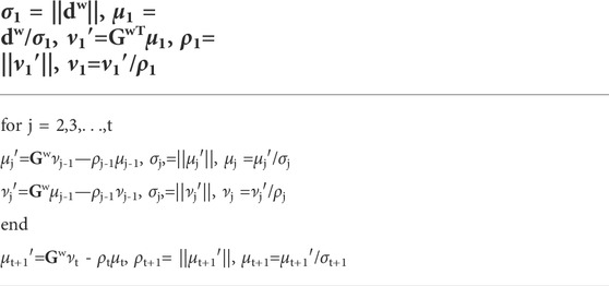
TABLE A1. Calculation algorithm of the Lanczos bidiagonalization.

With the suitable compression factor, t, this algorithm produces two matrices U_t = [μ₁, μ₂,…, μ_t]∈ℜ^M×t and V_t=[ν₁, ν₂,…, ν_t+1] ∈ℜ^N×(t+1) with orthonormal columns and a lower bidiagonal matrix B_t∈ℜ ^(t+1)×t which is define as follows:

${\mathbf{B}}_t=\left[\begin{array}{ccccc}{\rho }_1& & & & \\ {\sigma }_2& {\rho }_2& & & \\ & \ddots & \ddots & & \\ & & {\sigma }_{t-1}& {\rho }_{t-1}& \\ & & & {\sigma }_t& {\rho }_t\\ & & & & {\sigma }_{t+1}\end{array}\right](28)$

The aforementioned matrices are related to each other via the expression:

$\begin{array}{cc}{\mathbf{G}}^w{U}_t=V_{t+1}{\mathbf{B}}_t,& V_{t+1}{\mathbf{e}}_{t+1}=\frac{{\mathbf{d}}^w}{{\Vert {\mathbf{d}}^w\Vert }_2}\end{array}(29)$

where e_t+1∈ℜ^(t+1)×1 is the unit vector with first column equal to 1.

Adaptive Choice of ω

In the early iteration of the gravity inversion, the solution is not captured by the ill-conditioning. Therefore, a regularization parameter, λ, must be introduced. This parameter must satisfy:

$0\le \lambda \le {\sigma }_{\min }\left(\mathrm{A}\right)(30)$

where σ_min is the smallest singular value of A, which corresponds to G or B_t. If the value of the regularization parameter, λ_k, is known in the iteration k, the value of ω is obtained via the minimization of the GCV function with respect to w. The function has the following mathematical expression:

$\frac{\partial }{\partial \lambda }{\left(GCV\left(\omega ,\lambda \right)\right)|}_{\lambda ={\lambda }_k}=0(31)$

In the calculation, the optimal regularization parameter is not known. Therefore, the value of ω is calculated via λ_k = σ_min(A). In later iterations, the ill-conditioning of A appears and one cannot use the value of σ_min(A) to replace λ. A better approach is to adaptively consider

${\omega }_k=\mathit{mean}\left(\begin{array}{cccc}{\omega }_1& {\omega }_2& \dots & {\omega }_{k-1}\end{array}\right)(32)$

In the iteration, by using the average value of the previous value of ω. In this way, the earlier well-conditioned values can balance the effects of false condition number in the A matrix.