Instability simulation of the submerged anti-dip slope based on the CFD-DEM coupling method

More and more underwater-related geotechnical problems have arisen, but there is little research about the instability process of submerged anti-dip slopes. This study built the CFD–DEM coupling method based on the CFD solver OpenFOAM and the DEM solver PFC. The Ergun test was selected as the benchmark test to verify the accuracy of the coupling method, and the pressure drop predicted from the coupling method agreed well with the analytic solution. Then, we built a numerically submerged anti-dip slope model, and a special effort was made to study its instability characteristic. The flow of water will weaken the slope stability, and the birth of cracks will be accelerated. The drag force will restrain the toppling deformation, resulting in a deeper fracture surface. Then, we changed the joint thickness and joint angle to study its effect on slope stability. The collapse load increases with the joint thickness, and the form of toppling deformation changes from flexural failure to block failure. The collapse load increases with the decreasing joint dip, and the position of the damaged area becomes higher; the angle between the bottom fracture surface and the vertical line to joints becomes smaller with the decreasing joint dip.

1 Introduction

A considerable number of engineering constructions are observed along the river, along the coast, or even under the sea. These engineering constructions will make evident disturbances to the stratum structure and have a significant impact on the stability of water-related slopes, like 1) the Three Gorges Reservoir, 2) the exploitation of oil and gas resources in the Yellow River Delta, and 3) the exploitation of combustible ice. The instability of these slopes not only poses a great threat to people’s lives and artificial facilities but also leads to some catastrophic disasters (like tsunami and earthquake), which are also thought to be associated with these slopes (Ten Brink et al., 2009; Goff and Terry, 2016; Yavari-Ramshe and Ataie-Ashtiani, 2017; Tappin, 2021). The seepage can carry away different kinds of particles in the soil, causing gradual destabilization of the submerged soil structure (Bai et al., 2021a; Bai et al., 2021b). At present, research about the instability characteristics of water-related slopes is at its early stage.

According to the existing research, 33% of slope deformation is toppling deformation, and most huge and severe slope deformation failure occurs in anti-dip slopes (Huang, 2007). The obvious features of toppling deformation are as follows: 1) the formation of the flexural fracture surface usually takes quite a long time and 2) catastrophic failure will usually happen when this kind of slope is unstable. If toppling deformation occurs in submerged slopes, the swells from the rock mass will pose a major threat to passing ships. We must analyze the instability process of the submerged anti-dip slope.

The discrete element method (DEM) is capable of simulating large deformation of rock and soil mass, and the computational fluid dynamics (CFD) method is suitable for simulating the motion of the fluid. Many scholars have introduced CFD to calculate the mechanical action of water on rock and soil (Thallak et al., 1991; Bruno, 1994; Han et al., 2018; Dong et al., 2021; Zhang et al., 2021). The CFD–DEM coupling simulation will be an appropriate method to study water-related geotechnical problems.

Some researchers carried out this kind of research in particle flow code (PFC) through Cundall’s method (Han and Cundall, 2011, 2013). Wang et al. (2014) and Zhou et al. (2016) have utilized PFC2D to simulate the evolution process of hydraulic fracturing and systematically study the initiation, size, and the number of fractures. Crosta et al. (2015) combined PFC2D and a three-dimensional CFD program and studied the destruction of steep submarine slopes caused by the thermal decomposition of methane hydrate. Although the CFD grid is three-dimensional, the boundary conditions in the Y-direction of the grid are fixed to achieve two-dimensional CFD calculations. Mingjing et al. (2018) then considered the Magnus effect to further optimize the coupling method and studied submarine landslide in the methane hydrate enrichment area under the action of the seismic load. Gu et al. (2019) wrote a CFD solver through Python and realized the simulation of erosion caused by seepage in cohesive sand in PFC3D. Xiong et al. (2021) proposed a new fluid–solid coupling method in combination with the CFD software application OpenFOAM and the DEM software application LIGGGHTS-PUBLIC. After verifying the accuracy of the method, they studied the diffusion characteristics and mechanical behavior of seepage in discontinuous graded granular soil. Bai et al. (2022) utilized the smoothed particle hydrodynamics (SPH) method to simulate the heat transfer process in porous media at the pore scale, and a concise method was proposed to produce unsaturated media by simulating the wetting process in dry media.

Moreover, research about the CFD–DEM simulation of water-related geotechnical problems is fruitful, but there is little research about the submerged anti-dip slope. In this study, the CFD solver OpenFOAM will be introduced to cooperate with the DEM solver PFC, and the verification of the coupling method will be conducted through the Ergun test. Then, we will utilize the coupling method to study the instability process of the submerged anti-dip slope. The classical centrifuge test (Adhikary and Dyskin, 2007) will be built by the DEM software application PFC to verify the accuracy of the DEM model. Then, the coupling method will be utilized to set the DEM model in a fluid mesh to simulate the instability process of the submerged anti-dip slope.

2 CFD–DEM coupling method

2.1 Governing equation of the DEM

In the PFC3D, the motion of these rigid particles obeys Newton’s law of motion, and the time-step iteration of its motion equation adopts an explicit central difference format, without the need to establish a large stiffness matrix (Inc, 2016). The equations of translation and rotation are as follows:

$\begin{array}{c}\frac{\mathrm{d}{\overrightarrow{u}}_{\text{pi}}}{\mathrm{d}t}=\frac{{\overrightarrow{f}}_{\text{mech}}+{\overrightarrow{f}}_{\text{fluid}}}{m}+g,\\ \frac{\mathrm{d}{\overrightarrow{\omega }}_{\text{pi}}}{\mathrm{d}t}=\frac{\overrightarrow{M}}{I},\end{array}(1)$

where ${\overrightarrow{u}}_{pi}$ presents the velocity vector of particle i; t is the time; ${\overrightarrow{f}}_{\text{mech}}$ is the resultant force of the contact force and gravity; ${\overrightarrow{f}}_{\text{fluid}}$ is the fluid force applied on the particle i; $m$ is the mass of the particle i; $g$ is the acceleration of gravity; ${\overrightarrow{\omega }}_{\text{pi}}$ is the angular velocity vector of the particle i; $\overrightarrow{M}$ is the moment; and I is the moment of inertia.

2.2 Governing equation of CFD

In this study, the continuous fluid domain is discretized into cells, and the motion of the incompressible fluid with a constant density can be expressed by the locally averaged Navier–Stokes continuity equation:

$\begin{array}{c}\frac{\partial \left({\phi }_{\mathrm{f}}{\rho }_{\mathrm{f}}\right)}{\partial t}+\mathit{\nabla }\cdot \left({\phi }_{\mathrm{f}}{\rho }_{\mathrm{f}}{v}_{\mathrm{f}}\right)=0,\\ \frac{\partial \left({\phi }_{\mathrm{f}}{\rho }_{\mathrm{f}}{v}_{\mathrm{f}}\right)}{\partial t}+\mathit{\nabla }\cdot \left({\phi }_{\mathrm{f}}{\rho }_{\mathrm{f}}{v}_{\mathrm{f}}{v}_{\mathrm{f}}\right)=-\mathit{\nabla }p+F_b+{\phi }_{\mathrm{f}}{\rho }_{\mathrm{f}}g+{\phi }_{\mathrm{f}}\mathit{\nabla }\left(\mu \mathit{\nabla }{v}_{\mathrm{f}}\right),\end{array}(2)$

where ${\phi }_{\mathrm{f}}$ denotes the porosity of the fluid; $v_{\mathrm{f}}$ is the fluid velocity vector; ${\rho }_{\mathrm{f}}$ is the density of the fluid; $\mathit{\nabla }p$ is the fluid pressure gradient; and $g$ is the gravitational acceleration.

$F_b$ is the per unit body force of the fluid cell applied by particles in a fluid cell, which can be expressed as Eq. 3, where ${\overrightarrow{f}}_{\mathrm{d}\mathrm{r}\mathrm{a}\mathrm{g}}$ is the drag force and $V_{cell}$ is the volume of the fluid cell

$F_b=\frac{{\sum }_{i=1}^N{\overrightarrow{f}}_{\mathrm{d}\mathrm{r}\mathrm{a}\mathrm{g}}^i}{V_{cell}}.(3)$

2.3 Particle–fluid interaction

The ${\overrightarrow{f}}_{\text{fluid}}$ is the fluid–particle interaction force, which is made up of the drag force ${\overrightarrow{f}}_{\text{drag}}$ and another part from the fluid pressure. The part from the fluid pressure consists of the buoyancy force ${\overrightarrow{f}}_{\mathrm{b}}$ and the pressure gradient force ${\overrightarrow{f}}_{\nabla p}$ . Therefore, the ${\overrightarrow{f}}_{\text{fluid}}$ can be defined as follows:

${\overrightarrow{f}}_{\text{fluid}}={{\overrightarrow{f}}_{\mathrm{d}\mathrm{r}\mathrm{a}\mathrm{g}}+\overrightarrow{f}}_{\mathrm{b}}+{\overrightarrow{f}}_{\mathit{\nabla }p}.(4)$

As a particle may intersect more than one fluid element, the drag forces that the fluid exerts on the particles are distributed based on the fractional overlap between the particle and the fluid element. It should be noted that the fluid forces act on the centroid of particles, and the rotational moment will not be applied to the particles. The drag force ${\overrightarrow{f}}_{\mathrm{d}\mathrm{r}\mathrm{a}\mathrm{g}}$ is related to the porosity of the fluid element ${\phi }_{\mathrm{f}}$ :

${\overrightarrow{f}}_{\mathrm{d}\mathrm{r}\mathrm{a}\mathrm{g}}={{\overrightarrow{f}}_0{\phi }_{\mathrm{f}}}^{-\chi },(5)$

where ${\overrightarrow{f}}_0$ is the single particle drag force; $\chi$ is the empirical correction coefficient to expand the application scope of Eq. 5 in both high- and low-porosity fluid elements and a large range of Reynolds numbers (Di Felice, 1994; Xu and Yu, 1997).

Here, ${\overrightarrow{f}}_0$ is defined as follows:

${\overrightarrow{f}}_0=\frac{1}{2}{C}_{\mathrm{d}}{\rho }_{\mathrm{f}}\pi r^2\left|\overrightarrow{u}-\overrightarrow{v}\right|\left(\overrightarrow{u}-\overrightarrow{v}\right),(6)$

where $C_{\mathrm{d}}$ presents the drag coefficient and r is the radius of the particle.

$C_{\mathrm{d}}$ is defined as follows (Di Felice, 1994):

$C_{\mathrm{d}}={\left(0.63+\frac{4.8}{\sqrt{R{e}_{\mathrm{p}}}}\right)}^2,(7)$

where $R{e}_{\mathrm{p}}$ denotes the Reynolds number.

$\chi$ is expressed as follows (Xu and Yu, 1997):

$\chi =3.7-0.65\cdot \exp \left(-\frac{{\left(1.5-{\log }_{10}^{R{e}_p}\right)}^2}{2}\right).(8)$

The Reynolds number $R{e}_{\mathrm{p}}$ is presented as follows (Xu and Yu, 1997):

$R{e}_{\mathrm{p}}=\frac{2{\rho }_{\mathrm{f}}r\left|\overrightarrow{u}-\overrightarrow{v}\right|}{\mu }.(9)$

The buoyance force ${\overrightarrow{f}}_{\mathrm{b}}$ is defined as follows:

${\overrightarrow{f}}_{\mathrm{b}}=-\frac{4}{3}\pi r^3{\rho }_{\mathrm{f}}g.(10)$

The pressure gradient force ${\overrightarrow{f}}_{\mathit{\nabla }p}$ is defined as follows:

${\overrightarrow{f}}_{\mathit{\nabla }p}=\frac{4}{3}\pi r^3\mathit{\nabla }p.(11)$

The fluid–particle interaction force ${\overrightarrow{f}}_{\mathrm{f}\mathrm{l}\mathrm{u}\mathrm{i}\mathrm{d}}$ can also be expressed as follows:

${\overrightarrow{f}}_{\mathrm{f}\mathrm{l}\mathrm{u}\mathrm{i}\mathrm{d}}={{\overrightarrow{f}}_{\mathrm{d}\mathrm{r}\mathrm{a}\mathrm{g}}+\overrightarrow{f}}_{\mathrm{b}}+{\overrightarrow{f}}_{\mathit{\nabla }p}={\overrightarrow{f}}_{\mathrm{d}\mathrm{r}\mathrm{a}\mathrm{g}}+\frac{4}{3}\pi r^3\left(\mathit{\nabla }p-{\rho }_{\mathrm{f}}g\right).(12)$

2.4 Coupling procedure

The CFD–DEM coupling method is built based on the DEM solver Particle Flow Code 3D (version 6.0021) and the open source CFD package OpenFOAM (version 3.0). The CFD–DEM coupling flowchart is shown in Figure 1. The PFC3D contains the CFD module but does not have the CFD solver; the OpenFOAM package serves as the CFD solver for the fluid mesh built in PFC3D. The $t_{target}$ is the CFD–DEM integration frequency. Each time the PFC3D runs for $t_{target}$ physical time, the particle information is transferred to OpenFOAM via Python, and OpenFOAM is allowed to run for the same length of physical time, after which the fluid information in OpenFOAM is given to the PFC3D’s mesh.

FIGURE 1

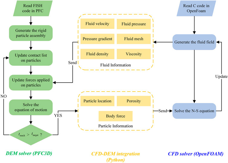
FIGURE 1. Coupling flowchart of the CFD–DEM method.

2.5 Benchmarking

A convincing CFD–DEM coupling method must pass the verification with the actual test (Pianet et al., 2007; Chen et al., 2011; Kloss et al., 2012; Zhao and Shan, 2013; Shan and Zhao, 2014; Li and Zhao, 2018). In this study, the Ergun test (Ergun, 1952) is selected as the benchmark test. In the Ergun test, the fluid flow through the granular column and the pressure drop ( $\Delta p$ ) across the granular bed are related to the superficial velocity $v_s$ . This relation is called the Ergun equation:

$\Delta p=\frac{150\mu H{\left(1-e\right)}^2}{d^2{e}^3}{v}_s+\frac{1.75Hp\left(1-e\right)}{d{e}^3}{v}_s\left|v_s\right|,(13)$

where H represents the height of the granular bed, d is the equivalent spherical diameter of the granular assembly, ρ is the fluid density, μ is the dynamic viscosity of the fluid, and e is the void fraction of the granular assembly.

As shown in Figure 2, the Ergun test model will be utilized to verify the accuracy of the CFD–DEM coupling method. The bottom (Figure 2B) is the inlet boundary of the Ergun test model, and Figure 2C is the velocity vector of the fluid mesh. The detailed parameters of the numerical Ergun Test is shown in Table 1.

FIGURE 2

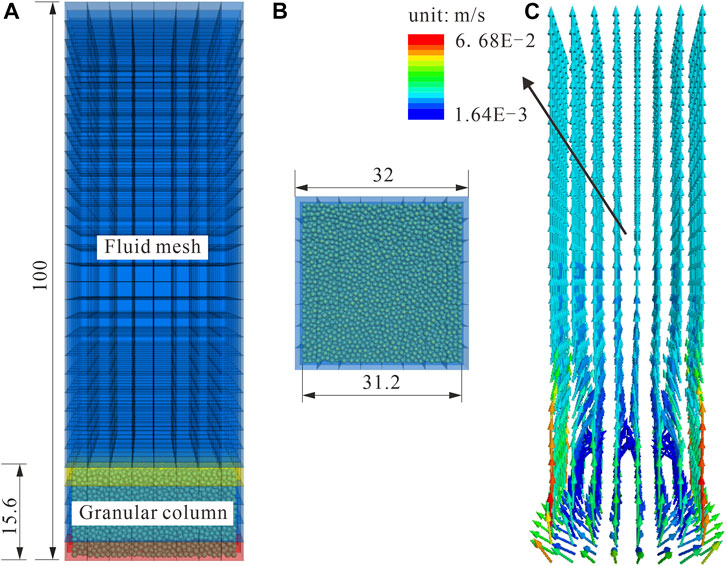
FIGURE 2. Ergun test model (unit: mm): (A) front view; (B) bottom view; and (C) fluid velocity vector.

TABLE 1

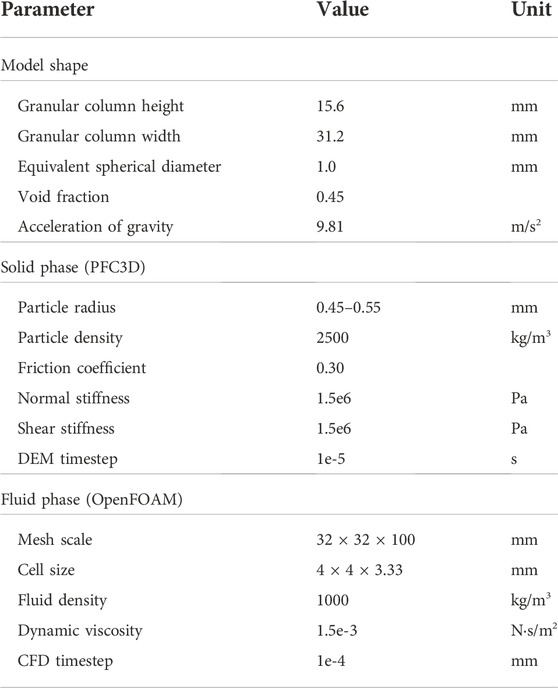
TABLE 1. Detailed parameters adopted in the numerical Ergun test.

2.6 Modeling procedure

i. A 31.2 × 31.2 × 15.6-mm cubic shape granular column was created whose void fraction was 0.45, and the particle radius was uniformly distributed in the range of 0.45–0.55 mm;

ii. A 32 × 32 × 100-mm cubic shape fluid mesh was generated, and the granular column was allowed to stand still in the fluid phase for 1 s;

iii. Superficial velocity was set in the bottom boundary of the fluid mesh, and the pressure drop was measured from the orange mesh to the yellow mesh (Figure 2A).

As shown in Figure 3, the pressure drop predicted from the CFD–DEM coupling method agrees well with the analytic solution (Ergun, 1952). Also, the accuracy of the coupling method is proven through this validation case. It should be noted that there will be no fluidization in this simulation as the granular bed is fixed.

FIGURE 3

FIGURE 3. Pressure drop contrast with the analytical solution (Ergun equation).

3 Submarine toppling simulation

3.1 Toppling simulation without water

In this part, a classic centrifuge test will be reproduced in the PFC3D to show DEM’s capability of accurately simulating toppling deformation and for a better comparison with the further submarine type.

3.1.1 Model description

This model is built based on the actual centrifuge test (Adhikary and Dyskin, 2007); its geometry and strength details are presented in Figure 4 and Table 2, respectively.

FIGURE 4

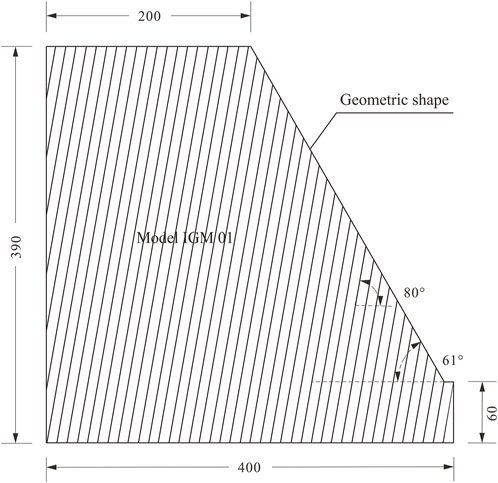
FIGURE 4. Geometrical details of Model IGM 01 (unit: mm).

TABLE 2

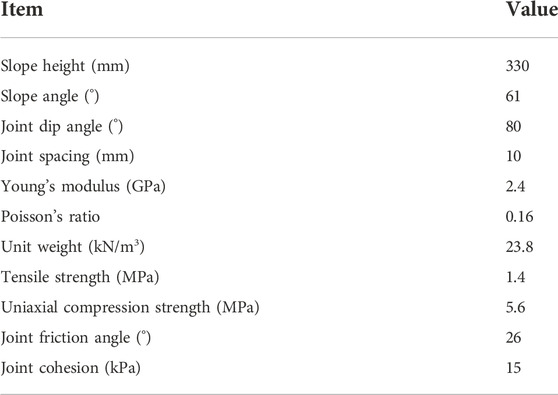
TABLE 2. Geometrical and strength parameters of IGM 01.

3.1.2 Micro parameter determination

The numerical model in the PFC is an assembly of bonded particles, and all inputted parameters are related to the physical characteristics of these microparticles or the contact model. However, we usually can get only the macro parameters (like Young’s modulus, Poisson’s ratio, and compression or tensile strength) through the laboratory test. These macro parameters cannot be inputted to PFC models directly. Through the numerical laboratory test, we can get the numerical macro physical characteristics and compare it with the actual characteristics to ensure the micro parameters. Before simulating toppling deformation in PFC3D, micro parameter calibration is an indispensable step. In order to reduce the length of the article, the details of the calibration part will not be shown in this study.

Numerical macro parameters can be obtained through the stress–strain curve (Figure 5); the comparison between the numerical and actual macro parameters is listed in Table 3. The difference between the numerical and actual macro parameters is acceptable, and the micro parameters (Table 4) are determined.

FIGURE 5

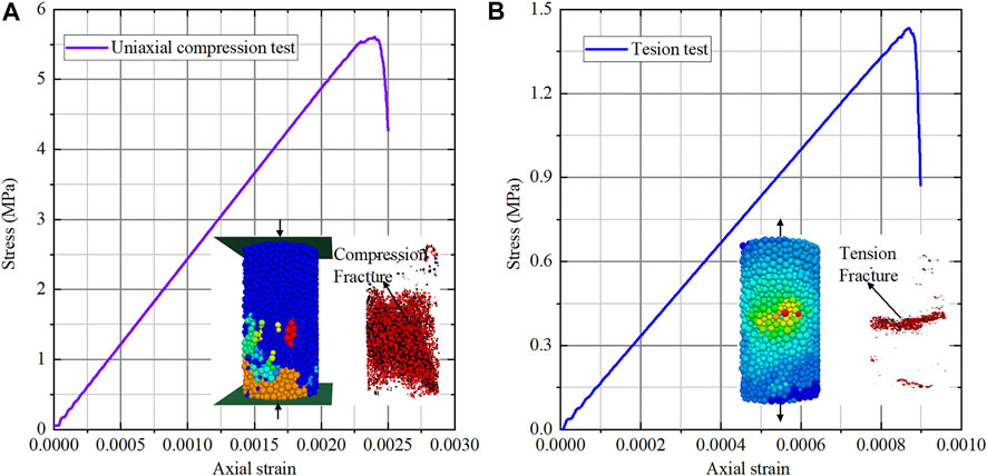
FIGURE 5. Simulated PFC3D failure in (A) UCS and (B) tension test.

TABLE 3

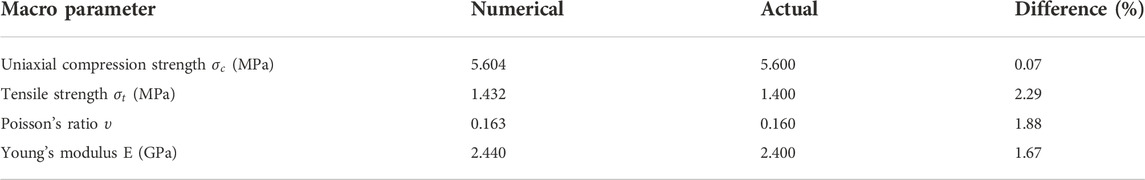
TABLE 3. Comparison of macro parameters from numerical and actual simulation.

TABLE 4

TABLE 4. Determined micro parameters.

3.1.3 Model setup

Because of the required high accuracy and low computing resource, many researchers have reproduced this centrifuge test in 2D cases (Alzo’ubi et al., 2010; Lian et al., 2018; Zheng et al., 2018). However, the coupling method in this study only supports 3D cases, and the 3D DEM simulation is quite computationally expansive. To save the computing resources, we decide to build this anti-dip slope in the pseudo 3D method. The slope model (Figure 6) is still built in 3D space, but the model length in the Y-direction is limited to the thickness of 2–3 particles, and two smooth walls are fixed in the model front and back to restrain displacement in the Y-direction. Although the pseudo-3D method is hard to show the change of the structure in the Y-direction, but the result of our referred physical test is also basically in the X- and Z-directions. The model is composed of 25,555 particles.

FIGURE 6

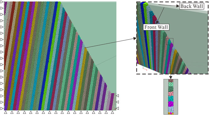
FIGURE 6. DEM model of the centrifuge test.

The gravity loading procedure is as follows.

(1) The anti-dip slope model is made to reach equilibrium at gravity 1 g.

(2) The model is allowed to run for a fixed amount of cycle steps (set to 5,000 in this model).

a) If no crack is generated, the gravity load is increased by 1 g and returns to step (2).

b) If a new crack is generated, the count of cycle steps in this stage returns to 0.

i. If no crack is generated in the subsequent cycle steps, the gravity load is increased by 1 g and returns to step (2).

ii. If a new crack is generated, it returns to (b).

(3) If the model is unable to jump out of step (2)-b)-ii, the gravity load at this point after the 2,000,000 cycle steps is the collapse load.

3.1.4 Verification

The simulation result is compared with the actual test and another numerical method in three aspects to prove the accuracy of DEM simulation:

(1) Angle of the failure surface: the failure surface in the actual centrifuge test was found to emanate from the slope toe and orient at an angle between 12° and 20°. The simulated failure surface is oriented at an angle of about 12.95°;

(2) Collapse load: the collapse load predicted from PFC3D is 92 g, and it is near to that in the original centrifuge test result (80–85 g);

(3) Horizontal displacement: as shown in Figure 7, the horizontal displacement–gravity load curve is compared with Adhikary’s test and the UDEC-TM method (Zheng et al., 2018). The horizontal displacement difference of points A and B between PFC3D simulation and Adhikary’s test is small, and the significant increase of horizontal displacement when gravity is about 35 is also captured. The accuracy is better than that of UDEC-TM. However, the accuracy of the DEM model is confirmed.

FIGURE 7

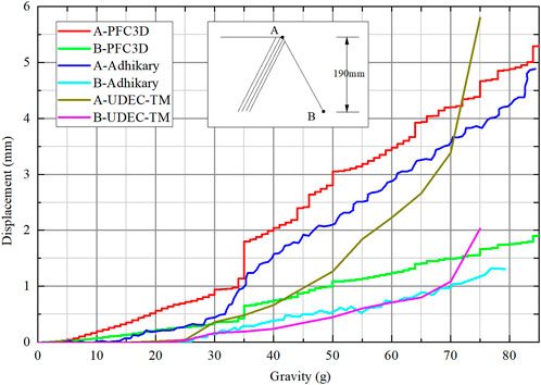
FIGURE 7. Displacement contrast with Adhikary’s test and the UDEC-TM method.

3.2 Instability simulation of the submerged anti-dip slope

As the accuracy of the coupling method and capability of simulating toppling deformation in the pseudo 3D method are confirmed, simulation of the instability process of the submerged anti-dip slope will be possible. Aiming to get a better comparison between the submerged type and natural land type, the slope model mentioned in section 3.1 will be set in static water (Figure 8) and simulated in the coupling method. The loading process is the same as that in section 3.1.

FIGURE 8

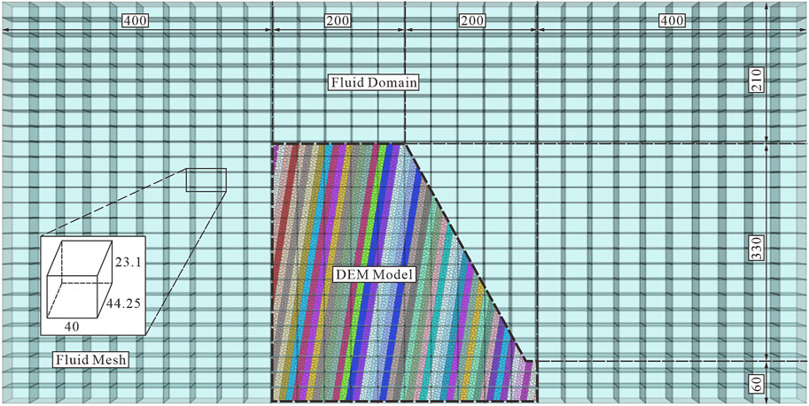
FIGURE 8. Schematic diagram of the submerged anti-dip slope (units: mm).

As the slope is set in water, the softening coefficient should be considered to achieve the deterioration of water on rock and soil materials. In this model, we select the softening coefficient as 0.49, and all macro parameters shown in Table 3 are multiplied by the softening coefficient. The new set of DEM and CFD parameters is listed in Table 5. It should be noted that the fluid mesh is of 3D type, but the fluid velocity boundary and fluid pressure boundary in the Y direction are set to 0.

TABLE 5

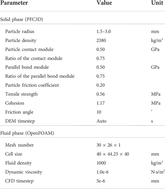
TABLE 5. Detailed parameters adopted in the submerged anti-dip slope model.

The post-failure result (rock fragments generated during the simulation) is shown in Figure 9; this model has run about 2,000,000 cycle steps, and the collapse load in the static water case is 72 g.

FIGURE 9

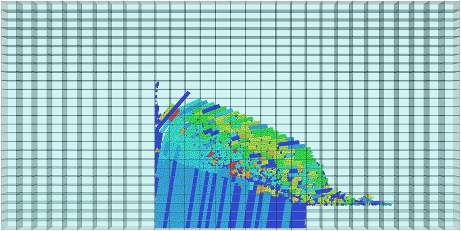
FIGURE 9. Post failure results in static water.

The energy evolution characteristics are shown in Figure 10:

FIGURE 10

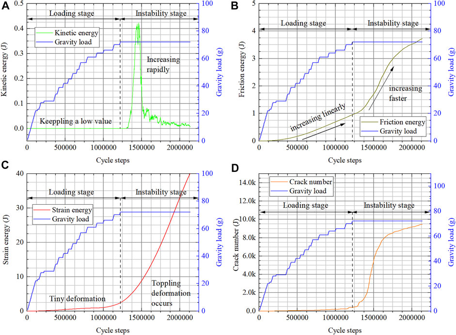
FIGURE 10. Energy evolution characteristics in the case of static water.

In Figure 10A, the kinetic energy is kept at a low value in the loading stage, and it increases rapidly after the gravity load reaches the collapse load. The friction energy (Figure 10B) increases linearly in the loading stage. As there is more interlayer friction motion when toppling deformation occurs, the friction energy increases faster when the gravity load reaches the collapse load. Large deformation will result in more strain energy. The strain energy (Figure 10C) increases quite slow when the slope is stable and increases quite fast when the slope is unstable. When the strain energy exceeds the tolerance of the rock mass, cracks will appear in the rock mass. Comparing Figure 10C,D , it is easy to find that the crack number is highly related to the strain energy.

4 Toppling stability analysis considering the water flow

The underwater environment is usually not as simple as the static water environment, and the flow of water also affects the stability of the slope. Considering the fluid flow in the instability simulation is necessary. In this section, we will set the hydraulic boundary to 1) v=0.5 m/s and 2) v=1 m/s to analyze the changes in toppling stability. It should be noted that the water flow direction is from left to right.

4.1 Instability process of the submerged anti-slope considering the water flow

To investigate the effects of the water flow on toppling deformation, four types of anti-dip slope models are selected for comparison, including 1) no water condition (shown in section 3.1), 2) static water condition (shown in section 3.2), 3) water flow velocity v=0.5 m/s, and 4) v=1.0 m/s.

The gravity loading process is shown in Figure 11A, and it is easy to see that the flow of water will decrease the stability of the slope. More details are shown in Figure 11B; the birth of cracks in the slope back is accelerated, and the increasing speed of the crack number in the loading process is faster. The flow direction of water may be from the back of the slope to the front, and the fluid force makes the slope more unstable. Thus, the horizontal displacement of points A and B (Figure 11C,D) increases faster.

FIGURE 11

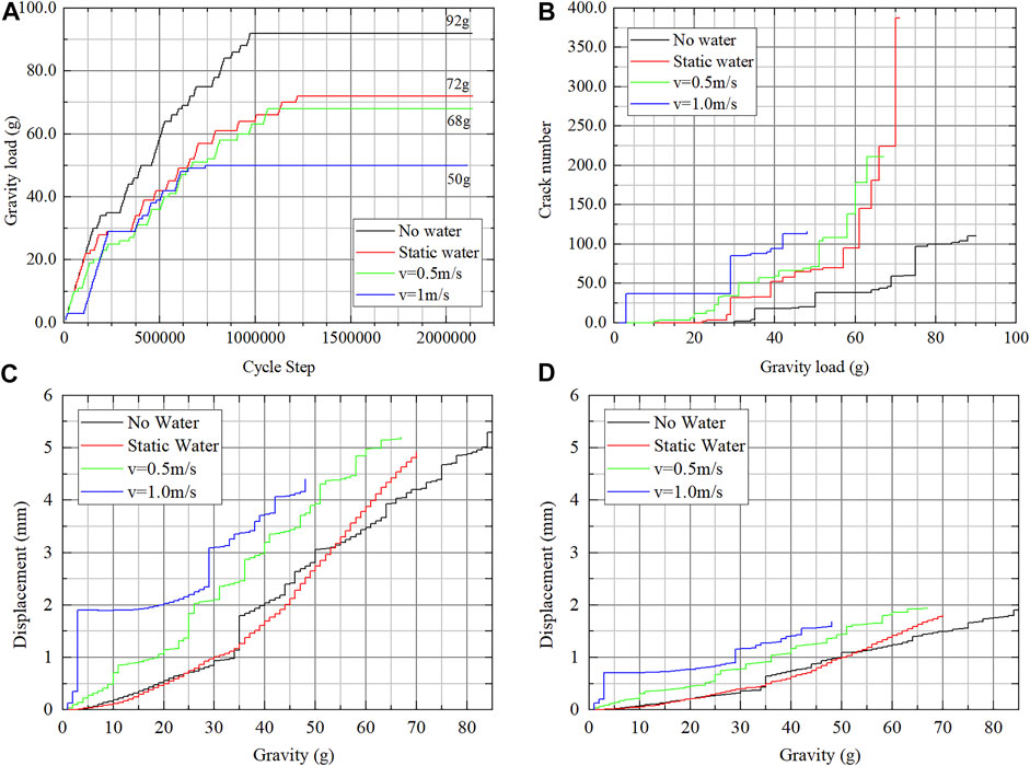
FIGURE 11. Contrast of the instability process: (A) collapse load; (B) crack number; (C) horizontal displacement of point A; and (D) horizontal displacement of point B.

The crack distribution of four types of models is shown in Figure 12. Measuring the angle between the vertical line of joints and the bottom fracture surface, we found that the angle becomes small after we set the model in water and that the water flow velocity has no obvious effect on this angle. The drag force from the fluid will restrain the toppling deformation, and every rock column should be fractured in a deeper position to get more gravity to overcome the drag force from the fluid.

FIGURE 12

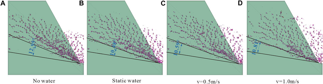
FIGURE 12. Crack distribution in every condition.

4.2 Effect of joint thickness on slope stability

In this section, we set the hydraulic boundary to v=0.75 m/s and change the joint thickness to study its effect on slope stability.

As shown in Figure 13A, the collapse load increases with the joint thickness, but the warning signs of slope failure have become less obvious. Not only does the growth rate of cracks decrease with the increasing joint thickness but also the number of peak cracks also decreases (Figure 13B).

FIGURE 13

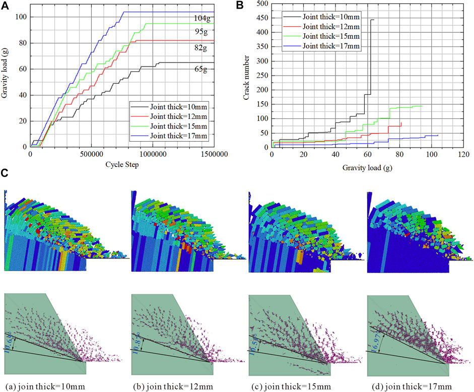
FIGURE 13. Effect of joint thickness on slope stability: (A) collapse load; (B) crack number; and (C) post-failure configuration.

It can be seen from Figure 13C that the form of toppling deformation has changed from flexural failure to block failure. Measuring the angle between the vertical line of joints and the bottom fracture surface, we found that the angle increases with the joint thickness. The reason may be that the mass of the rock column increases with the joint thickness, and the rock column can be fractured at a higher position.

4.3 Effect of the joint dip on slope stability

The hydraulic boundary is still set to v=0.75 m/s, and the joint dip is changed to study its effect on slope stability.

The relationship of the anti-dip slope stability between the joint dip is nonlinear (Xie et al., 2021). The water flow makes this relationship more complicated. Thus, in Figure 14A, there is no clear relationship between the collapse load and the joint dip. The initial growth rate of cracks decreases significantly after the joint dip is reduced, and the increasing crack stage is more concentrated when the gravity load is approaching the collapse load (Figure 14B).

FIGURE 14

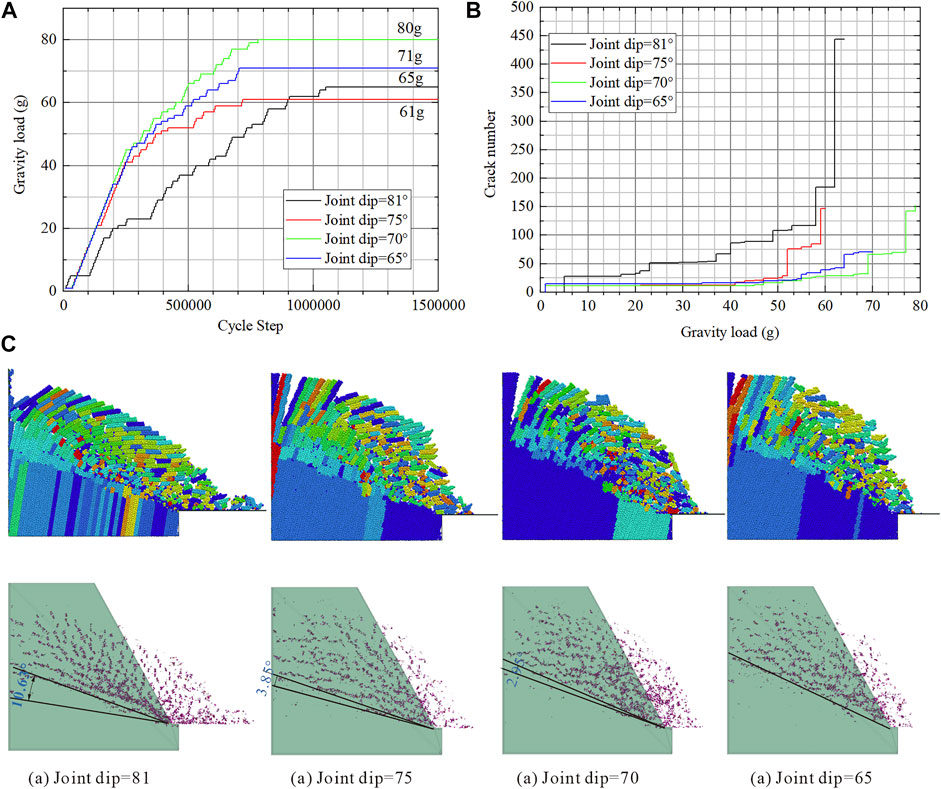
FIGURE 14. Effect of the joint dip on slope stability: (A) collapse load; (B) crack number; and (C) post-failure configuration.

As shown in Figure 14C, the position of the damaged area becomes higher with the decreasing joint dip. Measuring the angle between the vertical line of joints and the bottom fracture surface, the angle decreases evidently with the decrease of the joint dip and finally even perpendicular to the joint. From the point of view of the plane perpendicular to the joint, the position of the damaged area has become deeper. This may be because the smaller joint dip angle inherently increases the stability of the slope, coupled with the restrained effect from drag force, making rock columns need to be fractured in a deeper place.

5 Conclusion

This study combined the DEM software application PFC and the open source CFD package OpenFOAM to study the instability characteristics of the submerged anti-dip slope. The conclusions are as follows:

(1) The CFD–DEM coupling method is reliable. The pressure drop predicted from the coupling method agrees well with the analytic solution.

(2) The flow of water will reduce the slope stability. The specific manifestation is that the birth of cracks in the loading process is accelerated. The existence of water will apply the drag force to rock columns to restrain toppling deformation, and the rock columns will be fractured in a deeper position to get more gravity to overcome the resistance force.

(3) The collapse load increases with the joint thickness, and the failure type changed from flexural failure to block failure. The angle between the vertical line of joints and the bottom fracture surface gets larger with the joint thickness.

(4) The growth rate of cracks decreases significantly after the joint dip is reduced. The position of the damaged area becomes deeper with the decreasing joint dip. The relationship between the collapse load and joint dip is still nonlinear.

Data availability statement

The original contributions presented in the study are included in the article/Supplementary material. Further inquiries can be directed to the corresponding author.

Author contributions

All listed authors have made substantial, direct, and intellectual contributions to this work and have approved it for publication.

Funding

This research was funded by the National Natural Science Foundation of China (grant number: 51908482), the National Natural Science Foundation of China (grant number: 52068066), the Natural Science Foundation of Xinjiang Province (grant number: 2021D01C073), and the Graduate Innovation Project of Xinjiang Province (grant number: XJ2021G071).

Conflict of interest

LX was employed by the Xinjiang Research Institute of Building Science (Co., Ltd.).

The remaining authors declare that the research was conducted in the absence of any commercial or financial relationships that could be construed as a potential conflict of interest.

Publisher’s note

All claims expressed in this article are solely those of the authors and do not necessarily represent those of their affiliated organizations, or those of the publisher, the editors, and the reviewers. Any product that may be evaluated in this article, or claim that may be made by its manufacturer, is not guaranteed or endorsed by the publisher.

References

Adhikary, D. P., and Dyskin, A. V. (2007). Modelling of progressive and instantaneous failures of foliated rock slopes. Rock Mech. Rock Eng. 40 (4), 349–362. doi:10.1007/s00603-006-0085-8

CrossRef Full Text | Google Scholar

Alzo’ubi, A. K., Martin, C. D., and Cruden, D. M. (2010). Influence of tensile strength on toppling failure in centrifuge tests. Int. J. Rock Mech. Min. Sci. 47 (6), 974–982. doi:10.1016/j.ijrmms.2010.05.011

CrossRef Full Text | Google Scholar

Bai, B., Jiang, S., Liu, L., Li, X., and Wu, H. (2021a). The transport of silica powders and lead ions under unsteady flow and variable injection concentrations. Powder Technol. 387, 22–30. doi:10.1016/j.powtec.2021.04.014

CrossRef Full Text | Google Scholar

Bai, B., Nie, Q., Zhang, Y., Wang, X., and Hu, W. (2021b). Cotransport of heavy metals and SiO2 particles at different temperatures by seepage. J. Hydrology 597, 125771. doi:10.1016/j.jhydrol.2020.125771

CrossRef Full Text | Google Scholar

Bai, B., Wang, Y., Rao, D., and Bai, F. (2022). The effective thermal conductivity of unsaturated porous media deduced by pore-scale SPH simulation. Front. Earth Sci. (Lausanne). 10, 943853. doi:10.3389/feart.2022.943853

CrossRef Full Text | Google Scholar

Bruno, M. S. (1994). Micromechanics of stress-induced permeability anisotropy and damage in sedimentary rock. Mech. Mater. 18 (1), 31–48. doi:10.1016/0167-6636(94)90004-3

CrossRef Full Text | Google Scholar

Chen, F., Drumm, E. C., and Guiochon, G. (2011). Coupled discrete element and finite volume solution of two classical soil mechanics problems. Comput. Geotechnics 38 (5), 638–647. doi:10.1016/j.compgeo.2011.03.009

CrossRef Full Text | Google Scholar

Crosta, B., Sun, C., and Zhang, W. (2015). A study of submarine steep slope failures triggered by thermal dissociation of methane hydrates using a coupled CFD-DEM approach. Eng. Geol. 190, 1–16. doi:10.1016/j.enggeo.2015.02.007

CrossRef Full Text | Google Scholar

Di Felice, R. (1994). The voidage function for fluid-particle interaction systems. Int. J. Multiph. Flow 20 (1), 153–159. doi:10.1016/0301-9322(94)90011-6

CrossRef Full Text | Google Scholar

Dong, D. A., Ao, A., Wx, B., and Peng, D. C. (2021). CFD/DEM coupled approach for the stability of caisson-type breakwater subjected to violent wave impact. Ocean. Eng. 223, 108651. doi:10.1016/j.oceaneng.2021.108651

CrossRef Full Text | Google Scholar

Ergun, S. (1952). Fluid flow through packed columns. J. Mater. Sci. Chem. Eng. 48 (2), 89–94. doi:10.1016/0009-2509(53)80048-5

CrossRef Full Text | Google Scholar

Goff, J., and Terry, J. P. (2016). Tsunamigenic slope failures: The pacific islands ‘blind spot. Landslides 13 (6), 1535–1543. doi:10.1007/s10346-015-0649-3

CrossRef Full Text | Google Scholar

Gu, D. M., Huang, D., Liu, H. L., Zhang, W. G., and Gao, X. C. (2019). A DEM-based approach for modeling the evolution process of seepage-induced erosion in clayey sand. Acta Geotech. 14 (6), 1629–1641. doi:10.1007/s11440-019-00848-0

CrossRef Full Text | Google Scholar

Han, Y., and Cundall, P. A. (2011). Lattice Boltzmann modeling of pore-scale fluid flow through idealized porous media. Int. J. Numer. Methods Fluids 67 (11), 1720–1734. doi:10.1002/fld.2443

CrossRef Full Text | Google Scholar

Han, Y., and Cundall, P. A. (2013). LBM–DEM modeling of fluid–solid interaction in porous media. Int. J. Numer. Anal. Methods Geomech. 37 (10), 1391–1407. doi:10.1002/nag.2096

CrossRef Full Text | Google Scholar

Han, Z., Zhou, J., and Zhang, L. (2018). Influence of grain size heterogeneity and in-situ stress on the hydraulic fracturing process by PFC2D modeling. Energies 11 (6), 1413. doi:10.3390/en11061413

CrossRef Full Text | Google Scholar

Huang, R. (2007). Large-scale landslides and their sliding mechanisms in China since the 20th century. Chin. J. Rock Mech. Eng. 26 (3), 433

Google Scholar

Inc, I. C. G. (2016). PFC help document. Minneapolis, MN, USA: Itasca Consulting Group Inc.

Google Scholar

Kloss, C., Goniva, C., Hager, A., Amberger, S., and Pirker, S. (2012). Models, algorithms and validation for opensource DEM and CFD–DEM. Prog. Comput. Fluid Dyn. Int. J. 12 (2-3), 140–152. doi:10.1504/PCFD.2012.047457

CrossRef Full Text | Google Scholar

Li, X., and Zhao, J. (2018). Dam-break of mixtures consisting of non-Newtonian liquids and granular particles. Powder Technol. 338, 493–505. doi:10.1016/j.powtec.2018.07.021

CrossRef Full Text | Google Scholar

Lian, J.-J., Li, Q., Deng, X.-F., Zhao, G.-F., and Chen, Z.-Y. (2018). A numerical study on toppling failure of a jointed rock slope by using the distinct lattice spring model. Rock Mech. Rock Eng. 51 (2), 513–530. doi:10.1007/s00603-017-1323-y

CrossRef Full Text | Google Scholar

Mingjing, J., Zhifu, S., and Di, W. (2018). CFD-DEM simulation of submarine landslide triggered by seismic loading in methane hydrate rich zone. Landslides 15, 2227–2241. doi:10.1007/s10346-018-1035-8

CrossRef Full Text | Google Scholar

Pianet, G., Ten Cate, A., Derksen, J. J., and Arquis, E. (2007). Assessment of the 1-fluid method for DNS of particulate flows: Sedimentation of a single sphere at moderate to high Reynolds numbers. Comput. Fluids 36 (2), 359–375. doi:10.1016/j.compfluid.2005.12.001

CrossRef Full Text | Google Scholar

Shan, T., and Zhao, J. (2014). A coupled CFD-DEM analysis of granular flow impacting on a water reservoir. Acta Mech. 225 (8), 2449–2470. doi:10.1007/s00707-014-1119-z

CrossRef Full Text | Google Scholar

Tappin, D., R. (2021). Submarine landslides and their tsunami hazard. Annu. Rev. Earth Planet. Sci. 49, 551–578. doi:10.1146/annurev-earth-063016-015810

CrossRef Full Text | Google Scholar

Ten Brink, U. S., Lee, H. J., Geist, E. L., and Twichell, D. (2009). Assessment of tsunami hazard to the U.S. East Coast using relationships between submarine landslides and earthquakes. Mar. Geol. 264 (1), 65–73. doi:10.1016/j.margeo.2008.05.011

CrossRef Full Text | Google Scholar

Thallak, S., Rothenburg, L., and Dusseault, M. (1991). “Simulation of multiple hydraulic fractures in a discrete element system,” in The 32nd U.S. Symposium on rock mechanics (USRMS): OnePetro)

Google Scholar

Wang, T., Zhou, W., Chen, J., Xiao, X., Li, Y., and Zhao, X. (2014). Simulation of hydraulic fracturing using particle flow method and application in a coal mine. Int. J. Coal Geol. 121, 1–13. doi:10.1016/j.coal.2013.10.012

CrossRef Full Text | Google Scholar

Xie, L., Ge, Y., Zhang, J., Tan, S., Wang, B., Yan, E., et al. (2021). Geometric model for toppling-prone deformation of layered reverse-dip slope. Nat. Hazards (Dordr). 106 (3), 1879–1894. doi:10.1007/s11069-021-04516-z

CrossRef Full Text | Google Scholar

Xiong, H., Yin, Z. Y., Zhao, J., and Yang, Y. (2021). Investigating the effect of flow direction on suffusion and its impacts on gap-graded granular soils. Acta Geotech. 16 (3), 399–419. doi:10.1007/s11440-020-01012-9

CrossRef Full Text | Google Scholar

Xu, B. H., and Yu, A. B. (1997). Numerical simulation of the gas-solid flow in a fluidized bed by combining discrete particle method with computational fluid dynamics. Chem. Eng. Sci. 52 (16), 2785–2809. doi:10.1016/S0009-2509(97)00081-X

CrossRef Full Text | Google Scholar

Yavari-Ramshe, S., and Ataie-Ashtiani, B. (2017). A rigorous finite volume model to simulate subaerial and submarine landslide-generated waves. Landslides 14 (1), 203–221. doi:10.1007/s10346-015-0662-6

CrossRef Full Text | Google Scholar

Zhang, H., Zhang, B., Feng, H., Wu, C., and Chen, K. (2021). Macro and micro analysis on coal-bearing soil slopes instability based on CFD-DEM coupling method. PLoS ONE 16 (9), e0257362. doi:10.1371/journal.pone.0257362

PubMed Abstract | CrossRef Full Text | Google Scholar

Zhao, J., and Shan, T. (2013). Coupled CFD–DEM simulation of fluid–particle interaction in geomechanics. Powder Technol. 239, 248–258. doi:10.1016/j.powtec.2013.02.003

CrossRef Full Text | Google Scholar

Zheng, Y., Chen, C., Liu, T., Zhang, H., Xia, K., and Liu, F. (2018). Study on the mechanisms of flexural toppling failure in anti-inclined rock slopes using numerical and limit equilibrium models. Eng. Geol. 237, 116–128. doi:10.1016/j.enggeo.2018.02.006

CrossRef Full Text | Google Scholar

Zhou, J., Zhang, L., Braun, A., and Han, Z. (2016). Numerical modeling and investigation of fluid-driven fracture propagation in reservoirs based on a modified fluid-mechanically coupled model in two-dimensional particle flow Code. Energies 9 (9), 699. doi:10.3390/en9090699

CrossRef Full Text | Google Scholar