 Hao Li
 Shensen Hu*
 Shuo Ma
- College of Meteorology and Oceanology, National University of Defense Technology, Changsha, China
The day/night band channel on the JPSS series of satellites can detect the light and dark fringes of oceanic internal waves due to the reflectivity difference caused by the roughness of the sea surface under moon flare conditions. After optical imaging of oceanic internal waves, three image processing algorithms, i.e., the two-dimensional S transform, windowed Fourier transform, and wavelet packet transform methods, can be used to extract the parameter features of horizontal wavelength and propagation direction. The wave domain with known parameters is established through data simulation, and both image quality and image resolution are analyzed to assess algorithm performance in terms of relative errors. Finally, the experimental conclusions are verified in two examples of satellite observations in the South China Sea in 2020. We found that the windowed Fourier transform and wavelet packet transform methods exhibit better noise immunity, and the two-dimensional S transform method exhibits less calculation error and is more applicable to cases with small wavelengths. For large wavelengths, the windowed Fourier transform method is more suitable for calculating the horizontal wavelength, and the wavelet packet transform method is more suitable for calculating the propagation direction. By evaluating the applicability of these algorithms, this study provides a theoretical basis to support the analysis and processing of internal wave characteristics in future.
Introduction
Oceanic internal waves are fluctuations that are generated and propagated inside seawater due to seawater density stratification and disturbances to the seawater stratification. Internal oceanic waves exist in seasonal and permanent thermocline regions, and they cause changes in ocean temperature, salinity, and currents. They also have important impacts on turbulent mixing, underwater nutrient transport, and submarine navigation (Villamaña et al., 2017; Huarong et al., 2020). Internal waves can easily occur in continental shelves, straits, and marginal seas; thus, they are common in the Andaman Sea, South China Sea, White Sea, and Arabian Sea (Liu and D’Sa, 2019). In a layered ocean with internal waves, the density difference between the upper and lower layers is approximately three orders of magnitude less than that of the air-sea interface; thus, the horizontal scale and frequency of internal waves are frequently greater than those of surface waves, and the occurrence of these internal waves has many uncertainties, while satellite remote sensing can make continuous observations over a large area and a long period of time, and is often able to capture useful information about internal waves, so satellite remote sensing has been an important tool for observing oceanic internal waves (Liu et al., 2014).
Currently, the primary remote sensing instruments for internal wave observation are active microwave synthetic aperture radar (SAR) and the passive visible band radiometer. SAR interacts with the sea surface by emitting an electromagnetic pulse. It then uses the received backscattered energy to generate image. Internal waves change the microscale wave distribution on the sea surface through the flow field and form irradiated and scattered areas, which results changes in the roughness of the sea surface, which is manifested as bands of light and dark stripes in SAR images (Bao et al., 2020). SAR has the advantages of all-weather, all-day time and high spatial resolution, so SAR is often used in the research of internal wave observation (Liu, 2014). Similar to the SAR imaging mechanism, visible remote sensing is also imaged using sunlight reflected from the sea surface. Internal waves change the roughness of the sea surface, which affects the reflected light energy received by the satellite sensor; thus, the visible remote sensing is also expressed in a visible image as a set of alternating light and dark stripes (Jackson, 2007; Zhang et al., 2020; Ma et al., 2021). Visible band radiometers have high temporal resolution and wide spatial coverage, and can frequently observe internal wave phenomena in visible images. However, internal wave phenomena observed using traditional visible light remote sensing must be observed in the solar flare region. The solar flare area is an area where a satellite can receive the specular reflection of sunlight, which depends on the relative geometry of the Sun and the satellite, as well as several conditions, e.g., sea surface wind and waves (Christopher et al., 2010). Similar to solar flares, with the increasing sensitivity of satellite sensors, oceanic internal waves under moon flare conditions can able be observed (Miller et al., 2013; Hu, 2021; Meetei et al., 2020). Miller et al. used the day/night band (DNB) sensor of the Visible/Infrared Imaging Radiometer Suite (VIIRS) on the Suomi National Polar-orbiting Partnership (Suomi-NPP) to observe nighttime internal wave phenomena in the Celebes Sea region, and they demonstrated the potential application of DNB images to observe nighttime internal wave phenomenon (Miller et al., 2013).
Satellite remote sensing images can present the horizontal two-dimensional spatial distribution characteristics of the oceanic internal wave field; however, the dynamic parameters of oceanic internal waves, e.g., wavelength, amplitude, and propagation direction, cannot be obtained directly. Thus, it is necessary to extract the internal wave characteristic parameters from satellite images using algorithmic inversion (Gan et al., 2007; Chen et al., 2014; Chen et al., 2018; Hu et al., 2019; Zhang et al., 2021). Algorithms for inversion of internal wave parameters from satellite images mainly include Fourier transform, wavelet analysis, empirical mode decomposition (EMD), two-dimensional Stockwell transform (two-dimensional S transform), etc. The Fourier transform is a good reflection of the main wave information of internal wave, while the wavelet transform can obtain the information of internal wave waveform, but it is necessary to choose a suitable wavelet base function (Zhang et al., 2021). The EMD algorithm decomposes the signal into multiple eigenmode function components, and uses the maximum normalized variance to represent the characteristics of the internal wave signal (Chen et al., 2018). The two-dimensional S transform is a widely used spectral analysis technique capable of providing range-wavenumber localization of spatial profiles. This capability is well suited for texture feature analysis of various geophysical data (F. Gao et al., 2016; Hindley et al., 2016). Gan et al. used the fast Fourier spectral analysis method to extract the internal wave wavelength in the Bashi Channel region from the ERS-1 SAR image. The results show that the method has good consistency with the EMD and wavelet analysis methods (Gan et al., 2007). Chen et al. proposed a fully automatic extraction method of internal wave parameters in SAR images by using two-dimensional continuous wavelet transform, which can well locate the image areas where the internal waves are located, and automatically extract the internal wave parameters in these areas (Chen et al., 2014). Hu et al. used the two-dimensional S transform method to measure the internal wave wavelength and propagation direction in the DNB image. The horizontal wavelengths measured by the three observation experiments were concentrated at 3–15 km, and the propagation direction was 110°–170° counterclockwise. These results are generally consistent with the estimation result from the spacing pixel number (Hu et al., 2019). However, while these algorithms can invert the characteristic parameters of oceanic internal waves and achieve good results, different algorithms may affect the calculation results for the same internal wave phenomenon observed from different satellite images. Thus, a systematic analysis of the applicability of different algorithms in different cases is expected to effectively reduce the inversion errors caused by such algorithms.
The purpose of this research is to find suitable algorithms for satellite images of different qualities, and expect to more accurately extract the characteristic parameters of internal wave streaks in the images. The experiment focuses on both satellite image quality and spatial resolution to analyse the effects on the two-dimensional S transform, windowed Fourier transform, and wavelet packet transform methods. The wave domain with known parameters is established through data simulation, and the relative error is employed to characterize algorithm performance. The results of the simulation experiments are verified relative to known internal oceanic wave events, and the applicability of the three algorithms in different situations is identified, so that a good algorithm can be selected to reduce the calculation error which we expect to facilitate quantitative monitoring of oceanic internal waves in the future. The data used and the region where the experimentally selected internal wave events are located was described in Introduction, the characteristics of the three algorithms for calculating the internal wave parameters was described (Introduction), simulation experiments and DNB observation validation experiments were conducted in Introduction, respectively, and finally concluded with a summary of conclusions (Introduction).
Dataset and study area
As the first test satellite of the JPSS series satellite systems of polar-orbiting meteorological and environment, the NPP satellite carries a VIIRS/DNB channel that can provide relatively accurate nighttime radiance data through on-orbit radiometric calibration. The spectral response range of DNB is 0.5–0.9 μm, the dynamic range of the detected radiation reaches 107 orders of magnitude, the lowest detectable radiation intensity is approximately 0.02 nWcm−2·sr−1, and it has a swath width of approximately 3,000 km and spatial resolution of 742 m. Since its launch in 2011, the NPP satellite has demonstrated strong day and night observation capabilities. Up to 2017, the JPSS-1 operated, which serves as the official satellite of the NPP satellite and carried the same performance VIIRS/DNB channel. A number of studies have used DNB images to observe oceanic internal waves (Miller et al., 2013; Yang et al., 2014; Tensubam et al., 2021). The experimental data of nighttime observation of internal waves comes from the VIIRS/SDR data products publicly released by the Comprehensive Large Array-data Stewardship System (CLASS) under NOAA, using the NPP satellite version of the DNB channel data, which are respectively the Sensor Data SVDNB product and Geographic Information GDNBO product. They consist of 3,072×4064 pixels, and the SVDNB product provides the pupil irradiance and its quality mark information after operational radiometric calibration, and the GDNBO product provides the corresponding geometric information, e.g., latitude, longitude, lunar phase angle, and satellite zenith angle.
Oceanic internal waves occur frequently in the South China Sea region (Bai et al., 2014). This region exhibits vertical stratification of seawater with seasonal variation and has an underwater topography with obvious seabed undulation, thereby providing many observational events to study the generation and propagation of large amplitude internal waves (Farmer et al., 2011; Zhao et al., 2014). Internal waves in the South China Sea primarily occur in the area between the Luzon Strait and the South China continental shelf. These internal waves are stimulated by the interactions among tides and the terrain near the Luzon Strait, and then they propagate northwestward to the South China continental shelf (Liu and Hsu, 2004). In this study, we collected observation data from the NPP and JPSS-1 satellites transiting in the northern South China Sea in 2020, and we selected the nighttime DNB descending orbit data for March 9 and April 7 as experimental observation events, as shown in Figure 1. The extraction of internal wave characteristic parameters by the algorithm is essentially an application of image processing technology to internal wave research. It is assumed that the two internal wave events used in the experiments, as long as the internal wave streak features are clearly presented on the satellite images and all three algorithms are able to extract the internal wave parameters accurately for the original images, it means that the internal wave events do not affect the performance of the algorithms and have no impact on the experimental conclusions.
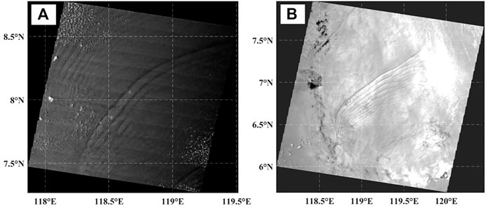
FIGURE 1. Nighttime DNB images of oceanic waves occurring in the South China Sea acquired by (A) the NPP satellite on 7 April 2020 at 17:23 UTC and (B) the JPSS-1 satellite on 9 March 2020 at 17:18 UTC.
Oceanic internal wave algorithms
Two-dimensional S transform
The two-dimensional S transform algorithm has been widely used in medical image analysis and mechanical exploration since its introduction in 1996. In 2016, Hindley et al. introduced the two-dimensional S transform algorithm to atmospheric and oceanic sciences by processing bright temperature images to analyze atmospheric gravity wave features (Hindley et al., 2016). The two-dimensional S transform algorithm has a strong ability to process and analyze two-dimensional digital image signals. For a two-dimensional spatial image
Here,
From Eqs 1, 2, the horizontal wavelength and propagation direction of the oceanic internal waves can be obtained as follows.
Here,
Windowed fourier transform
The two-dimensional discrete windowed Fourier transform method is a two-dimensional form of short-time Fourier transform. The short-time Fourier transform is one of the most commonly used methods for time-frequency analysis because it makes up for the lack of time domain information in the basic Fourier transform method by including a time window to obtain the frequency characteristics at a certain time (Li et al., 2019). The two-dimensional discrete windowed Fourier transform is an extension of the one-dimensional time domain into the two-dimensional discrete space domain. This extension allows us to obtain information in both the spatial and wave number domains, e.g., we can find the wave number information in a particular space. The two-dimensional discrete windowed Fourier transform final expression is given as follows.
Here, the corresponding form of the rectangular window is expressed as follows.
The windowed Fourier transform method in the wave number domain can achieve greater computational efficiency. As
Wavelet packet transform
A wavelet is a function defined in finite time with an average value of zero amplitude, finite duration, and abrupt frequency and amplitude. Wavelet transform can decompose a signal into a series of wavelet functions through the translation and scaling of the parent wavelet; thus, it can characterize the local characteristics of the signal in both the time and frequency domains (Wu et al., 2012). Let the two-dimensional image be
Here, the function
However, the wavelet transform algorithm continuously decomposes the low-frequency components of the signal and does not decompose the high-frequency components. To decompose the complete spectrum of the signal and obtain a particular frequency component from the signal, the high-frequency components of the signal must be decomposed further, which introduces the concept of wavelet packet transform (Xu et al., 2021). Based on the wavelet transform, the wavelet packet transform allows for multi-level decomposition of both the low-frequency and high-frequency components of the signal, which allows for finer frequency resolution in the high-frequency part.
Simulation experiments
The spatial resolution and imaging quality of remote sensing instruments are not the same; thus, the images obtained by different satellite sensors to observe the same internal wave phenomenon may also differ. In addition, the actual satellite observation of internal waves requires spatial geometric correction of the satellite image, from which partial images containing oceanic internal wave streak features are intercepted. After resampling, the resolution of the local image differs from that of the original image, and the change in spatial resolution also causes changes to the spatial wavelength of the oceanic internal wave in the image. Thus, it is necessary to evaluate algorithm performance on different satellite images for oceanic internal wave features in order to determine whether there is any impact on the results of the internal wave calculations.
The truth value of internal wave characteristics of satellite images cannot be obtained in large quantities to analyze the general rule, and there are many factors affecting the algorithm to extract internal wave parameters. Thus, this study draws on the analysis method of gravitational waves by Hindley et al., in 2016, using the simulation wave domain for analysis (Hindley et al., 2016). The analysis factor is used as the only independent variable through the control variable method and the remaining factors that may influence it are set as uniform parameters. Simulation experiments were conducted to analyze the effect of the independent variables on the performance of the algorithm by gradually adjusting the parameters of the independent variables for a known wave domain, without changing the other parameter settings. The experiment mainly focuses on image quality and image resolution as independent variables for two research analyses, where image quality is achieved by adding random noise to the image. Since image resolution affects the spatial wavelength of the internal wave, the spatial wavelength of the internal wave (represented by the number of image pixel intervals) is characterized as the image resolution for simulation experiments. The relative errors in the calculation of the horizontal wavelength and propagation direction are used to characterize the performance of the algorithm by comparing the calculated results of the internal wave streaks in the simulated wave domain with the true values of the set parameters. The calculation equation of relative error is expressed as follows:
where
Image quality analysis
The signal-to-noise ratio SNR, as the ratio of the signal S to the noise R, can reflect the blurring degree of the image. In practical applications, the image quality can be obtained by the SNR (Zhang et al., 2013). The image quality analysis experiment in this study were performed by adding random noise to change the image quality. Here, let the original image be
where
That is, the SNR and the noise ratio
To ensure that no other variables deteriorate the performance of the algorithm, the original image must satisfy the two-dimensional S transform, the windowed Fourier transform, and the wavelet packet transform methods with small computational errors. The calculation errors of these three algorithms changes successively by gradually superimposing random noise, as shown in Appendix Figure A1. To avoid the experimental contingency of the calculation results, the average value of 100 simulation experiments is used as the final experimental result, and this average value is compared to the set true value to obtain the relative error of the calculation under different random noise conditions, as shown in Figure 2.
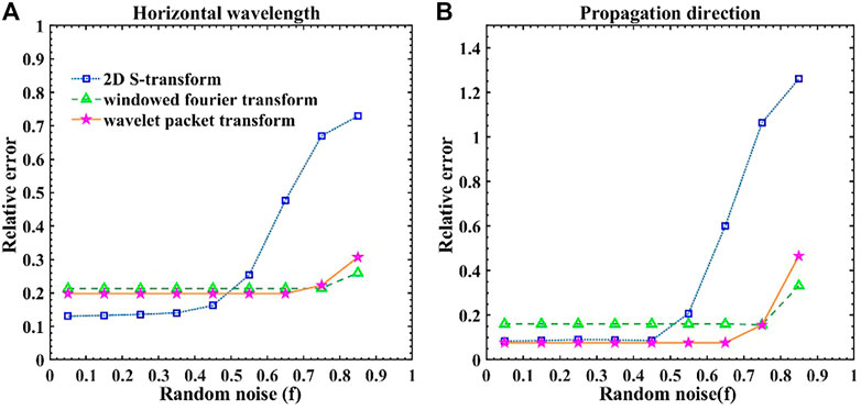
FIGURE 2. Computational errors of oceanic internal wave characteristics under different noise: (A) horizontal wavelength and (B) propagation direction.
Figure 2A shows the calculation errors of the three algorithms in the horizontal wavelength under different noise conditions. The calculation errors of the three algorithms are essentially constant below 0.4 noise. As can be seen, the two-dimensional S transform method has the smallest relative error (approximately 0.13), and the windowed Fourier transform and wavelet packet transform methods exhibit similar relative errors (approximately 0.2). When the random noise is greater than 0.4, the calculation error of the two-dimensional S transform method changes first, and as the noise increases, the calculation error of the two-dimensional S transform method changes greatly. With the wavelet packet transform method, the calculation error changes after the random noise becomes greater than 0.7. With the windowed Fourier transform method, the calculation error changes when the random noise is greater than 0.8, and the range of change is small in this case. Figure 2B shows the calculation errors of the three algorithms in the propagation direction under different noise conditions. As can be seen, the calculation errors of the two-dimensional S transform and wavelet packet transform methods are smaller and similar when the noise is below 0.5, and the relative errors are all approximately 0.1. When the noise becomes greater than 0.4, the calculated results of the two-dimensional S transform method change first, and the relative error increases to 0.2. The calculated results of the wavelet packet transform and windowed Fourier transform methods are similar to those shown in Figure 2A, i.e., they change only after the random noise reaches 0.7 and 0.8, respectively, and the relative error increases by a small margin.
As shown in Figure 2, all three algorithms exhibit relatively stable calculation performance when the random noise is less than 0.4. When the algorithm performance is stable, the two-dimensional S transform method demonstrates the smallest calculation error for both the horizontal wavelength and propagation direction. Although the calculation errors of the windowed Fourier transform and wavelet packet transform methods are relatively larger, the noise immunity of these algorithms is better than that of the two-dimensional S transform method. Thus, when the image quality is good, it is preferable to select the two-dimensional S transform algorithm to calculate the characteristics of internal waves. The windowed Fourier transform and wavelet packet transform methods are recommended when the image quality is poor, which may affect the observed internal wave characteristics.
Image resolution analysis
The horizontal wavelength of an internal wave in a satellite image is calculated from the number of pixels separating the two wave peak lines, and the number of pixels obtained for different spatial resolutions of the image will vary. Thus, for an internal wave event with the same actual wavelength, different image spatial wavelengths may be obtained. The simulation experiment takes the image space wavelength as an independent variable to characterize different image space resolutions. In this experiment, the relative errors in the calculation of spatial wavelengths within 0–50 pixels using the two-dimensional S transform, windowed Fourier transform, and wavelet packet transform methods were analyzed by building a random wave domain with 101
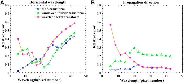
FIGURE 3. Computational errors of oceanic internal wave characteristics at different wavelengths: (A) horizontal wavelength (B) propagation direction.
Figure 3A shows the calculation errors of the three algorithms at different wavelengths for the horizontal wavelengths. As can be seen, the calculation error of the two-dimensional S transform method increases monotonically with increasing wavelength. The calculation errors of the windowed Fourier transform and wavelet packet transform method decrease with increasing wavelength when the wavelength is less than 20 pixels, and the errors increase with increasing wavelength when the wavelength is greater than 20 pixels. When the wavelength is less than 10 pixels or greater than 30 pixels, the calculation error of the two-dimensional S transform method is the smallest. When the wavelength is 10–20 pixels, the calculation errors of all three algorithms are relatively similar, and when the wavelength is 20–30 pixels, the calculation error of the windowed Fourier transform method is the smallest. Figure 3B shows the calculation errors of the three algorithms in the propagation direction at different wavelengths. As can be seen, the calculation errors of the wavelet packet transform method in the propagation direction decrease with increasing wavelength. When the wavelength is greater than 20 pixels, the calculation errors of the wavelet packet transform method are relatively consistent with those of the two-dimensional S transform method. The calculation errors of the windowed Fourier transform and two-dimensional S transform methods increase with increasing wavelength when the wavelength is less than 20 pixels, and they calculation errors decrease with increasing wavelength when the wavelength is greater than 20 pixels. However, the calculation error of the two-dimensional S transform method is small, and the change with wavelength is not obvious.
As shown in Figure 3, the two-dimensional S transform method exhibits the most stable performance among the three algorithms, and the error is relatively small. When the wavelength is small (i.e., the number of pixels is less than 20), it is better to use the two-dimensional S transform method to calculate the horizontal wavelength and propagation direction. In contrast, when the wavelength is large (i.e., the number of pixels is greater than 20), it is better to use the windowed Fourier transform method to calculate the horizontal wavelength, and either the wavelet packet transform method or two-dimensional S transform method should be used to calculate the propagation direction.
Actual satellite measurement data
Image quality analysis
An internal wave event that occurred in the South China Sea region (eight to nine N, 118–119 E) on 7 April 2020 was selected to verify the analysis of image quality in the simulation experiment. Here, we simulated different satellite sensors capturing low light images of different image quality by adding random noise to the original satellite images, as shown in Figure 4. Figure 4A shows the original image without additional noise, and Figures 4B, D show the corresponding images with random noise of 0.2, 0.4, and 0.6, respectively. From the characteristics of internal wave fringes shown in Figure 4, we find that the image appears blurred to varying degrees until the internal wave feature fringes in Figure 4D are nearly unrecognizable. The internal wave phenomena in Figure 4 can be handled by drawing software such as Photoshop to make a tangent to the maximum crest line of the internal wave at the pixel level and judge the propagation direction based on the tangent tilt angle, while the actual wavelength can be handled by Hu et al. through the estimated value of the number of pixels spacing the internal wave crest line (Hu et al., 2019), which can be summarized as follows:
Where
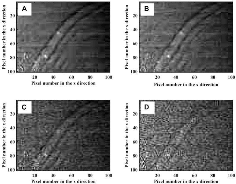
FIGURE 4. DNB image of internal wave phenomenon in the South China Sea region on 7 April 2020(8.0–9.2N, 118.2–119.4E), (A) is the original image without any noise added, (B) is the image with 0.2 random noise added on the basis of (A), (C) is the image with 0.4 random noise added on the basis of (A), (D) is the random noise image with 0.6 added on the basis of (A).
According to formula (11), the four partial images are all composed of 201 × 201 pixels. After performing spatial geometric correction using the latitude and longitude information, the approximate spatial resolution of the images is 662 m. Thus, the maximum spatial wavelength of the internal wave fringes in the figure (i.e., the maximum pixel interval between the two wave crest lines) is 10, the actual wavelength is about 6.6 km, and the propagation direction is −50°.
Here, to assess the effect of image quality on algorithm performance, we verify that the two-dimensional S transform, windowed Fourier transform, and wavelet packet transform methods can calculate the internal wave characteristic parameters accurately without additional noise. The three algorithms were used to calculate the horizontal wavelength and propagation direction of the internal wave fringes shown in Figure 4A, and the calculation results are shown in Figure 5. As shown in Figure 5, the internal wave phenomenon is clearly characterized in the images, where Figures 5(A) to 5(C) show the horizontal wavelengths calculated by the two-dimensional S transform, windowed Fourier transform, and wavelet packet transform methods, respectively. Here, by averaging the values of multiple points in the internal wave region, we find that the horizontal wavelengths are 8.93, 8.86, and 8.83, respectively, and the actual wavelengths calculated by the algorithm are about 5.91 km, 5.87 km and 5.85 km when combined with the image resolution. Combined with Eq 8, we can thus obtain the relative errors of this internal wave event as 0.10, 0.11, and 0.11 respectively. In contrast, the relative errors of the simulation experiments for the horizontal wavelengths are 0.13, 0.18, and 0.19, respectively, when no random noise is added. Figures 5D, F show the propagation directions calculated by the three algorithms with values of −53.97°, 47.49° and −45°, respectively. Also, according to formula (8), the relative errors are 0.07, 0.05, and 0.10, respectively, and the relative errors in the propagation directions calculated in the simulation experiments are 0.08, 0.08, and 0.16, respectively. Thus, in the absence of random noise, the calculation results are essentially consistent with the simulation results.
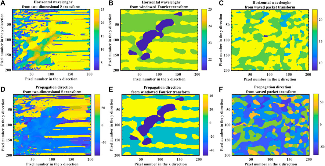
FIGURE 5. Horizontal wavelength internal wave without noise (Figure 4) calculated by (A) two-dimensional S transform, (B) windowed Fourier transform, and (C) wavelet packet transform, and propagation direction of internal wave without noise (Figure 4) calculated by (D) two-dimensional S transform, (E) windowed Fourier transform, and (F) wavelet packet transform.
By gradually adding image noise to the original satellite image, the target features are covered up, which reduces the algorithm’s calculation effect. In this experiment, the three algorithms were used to calculate the internal wave fringe characteristics in Figure 4, and the calculation results are given in Table 1. As shown in Table 1, the degree noise immunity of the two-dimensional S transform method is poor, and a large calculation error occurs in the horizontal wavelength and propagation direction of wave (c). In addition, when the image noise reaches 0.4 or greater, the computational performance of the two-dimensional S transform method changes, and the computational error continues to increase as the noise increases. In contrast, the windowed Fourier transform and wavelet packet transform methods exhibit better noise immunity. For the calculation error of the horizontal wavelength, the windowed Fourier transform methods maintains an error of 0.11, and the wavelet packet transform maintains an error of 0.12. For the propagation direction, the windowed Fourier transform and wavelet packet transform methods exhibit calculation errors of 0.05 and 0.10, respectively. Until the wavelet packet transform result changes at wave (d), the calculation performance deteriorates when the image noise becomes greater than 0.6. Through the above analysis, we find that the calculation error in terms of propagation direction is less than that of the horizontal wavelength. The two-dimensional S transform method demonstrates relatively poor noise immunity, while the windowed Fourier transform method demonstrates the best noise immunity. Overall, the calculated results are essentially consistent with the simulation results.
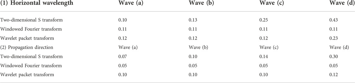
TABLE 1. Calculation errors of internal wave fringe in Figure 4 relative to (A) horizontal wavelength and (B) propagation direction.
Image resolution analysis
To verify the analysis of the wavelength of the internal wave in the simulation experiment, an internal wave event that occurred in the South China Sea region (5.8–7.8 N, 118–120 E) on 9 March 2020 was considered to perform geometric correction according to the latitude and longitude information of the pixel points to obtain different partial low light images at latitude and longitude, as shown in Figure 6. Here, the number of pixels in the resampled partial image is changed compared to the original image; thus, the spatial resolution of the partial image differs. The spatial resolution of the image changes the spatial wavelength (expressed as the number of pixels) that causes the internal waves in the image. The approximate spatial resolution of each partial image is calculated according to the rule that the actual distance difference is 111 km for every 1° difference in latitude. Figures 6A, D show that the image resolution is 148 m, 370 m, 518 m, and 740 m, respectively.
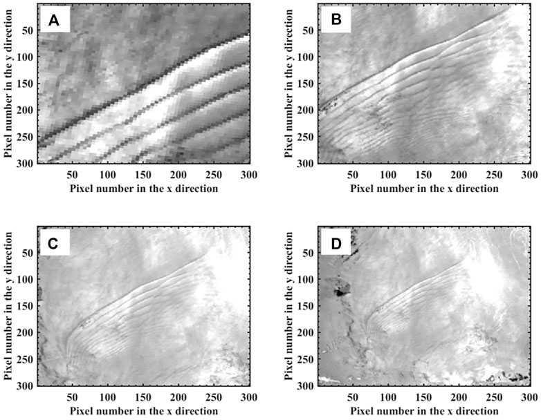
FIGURE 6. DNB images of internal wave phenomena in the South China Sea region on 9 March 2020 (5.8–7.8N, 118–120E). The spatial resolution of (A) is 185 m, (B) is 370 m, (C) is 518 m and (D) is 740 m.
The Canny algorithm (Canny, 1986) is used for image edge detection in Figure 6, and the peak line of the extracted internal wave in the image is shown in Figure 7. Here, the tangent line is obtained from the peak line, and the vertical distance between the two tangent lines is calculated manually as the spatial wavelength of the internal wave. According to the calculation, the spatial wavelengths of the internal waves in Figure 7 are 40, 16, 12, and eight pixels, respectively. Combined with the spatial resolution of each image, the actual wavelength of the internal waves is calculated as approximately 6 km. Three algorithms based on image processing is based on the spatial wavelength of the internal wave, and different spatial wavelengths may change the performance of the algorithm.
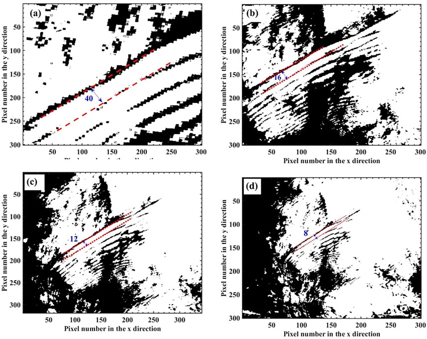
FIGURE 7. The peak line and spatial wavelength of the internal wave shown Figure 6 were extracted. The spatial wavelengths are (A) 40 pixels, (B) 16 pixels, (C) 12 pixels, and (D) eight pixels.
The four internal wave examples with different spatial resolutions in Figure 6 are calculated by the three algorithms. In Table 2, Eq 1 shows the horizontal wavelength calculation errors, and (2) shows the propagation direction calculation errors. As can be seen, the spatial wavelengths from waves (a) to (d), which represent the four wavelength cases selected with the wavelength distribution in the simulation experiment, decrease gradually. For the horizontal wavelength, the calculation error of the two-dimensional S transform method decreases with wavelength decreases, and the windowed Fourier transform and wavelet packet methods are more suitable for calculating internal wave cases with wavelengths in the range of 15–25 pixels, e.g., wave (b). In terms of the propagation direction, the calculation error of the two-dimensional S transform method is generally small, the calculation error of the windowed Fourier transform method decreases with wavelength decreases, and the calculation error of the wavelet packet transform method increases with wavelength decreases. The calculated results shown in Table 2 are in general agreement with the simulation results, and validate the conclusions of the image resolution analysis to a certain extent.

TABLE 2. Calculation errors of (a) horizontal wavelength and (b) propagation direction for the internal wave case shown in Figure 7.
Discussion and conclusion
The internal wave algorithm is an analysis and processing technology for satellite images that converts the spatial domain of the image into a frequency domain and uses a window function to extract feature information. As the window function varies, the effect of the algorithm to extract the internal wave parameters will also be different. The motivation of this study is to investigate whether differences between different low light images affect the calculation results of internal wave algorithms, i.e., the two-dimensional S transform, windowed Fourier transform, and wavelet packet transform algorithms. Simulation experiments were performed to analyze the effects of image quality and image resolution on the calculation of the horizontal wavelength and propagation direction of the internal wave, respectively, and the relative error compared to the known true value was considered to characterize algorithm performance. In addition, the applicability of the two-dimensional S transform, windowed Fourier transform, and wavelet packet transform methods were summarized for different situations. Finally, two internal wave events that occurred in the South China Sea region in 2020 were investigated to simulate the same internal wave characteristic streak images observed by different satellite sensors by adding random noise and pixel resampling to the DNB images, and the computational results of the three algorithms were compared to the simulation results to verify the accuracy of the simulation experiments.
The image quality analysis demonstrated that the two-dimensional S transform, windowed Fourier transform, and wavelet packet transform methods exhibited relatively stable calculation errors when the image noise was less than 0.4. For the horizontal wavelength calculation, the two-dimensional S transform method showed the smallest calculation error. For the propagation direction calculation, the two-dimensional S transform and wavelet packet transform methods exhibited the smallest calculation errors, and the results of these methods were similar. In practical applications, the noise ratio value in this experiment can be obtained by evaluating the SNR of satellite images, so as to select an appropriate algorithm. In general, when image quality is good, it is better to select the two-dimensional S transform algorithm. However, the noise immunity of the two-dimensional S transform method is poor, and the noise immunity of the windowed Fourier transform and wavelet packet transform methods is better than that of the two-dimensional S transform. Thus, when the quality of the satellite image is poor, it is recommended to select the windowed Fourier transform or wavelet packet transform method.
The image resolution analysis demonstrated that the two-dimensional S transform method generally exhibited the most stable performance among the three algorithms, and the error of this method was relatively small. Thus, when the wavelength is small, it is recommended to use the two-dimensional S transform method to calculate the horizontal wavelength and propagation direction. In contrast, when the wavelength is large, it is better to use the windowed Fourier transform method to calculate the horizontal wavelength and use the wavelet packet transform or two-dimensional S transform method to calculate the propagation direction. Note that the spatial wavelength size of the internal wave is determined relative to the number of pixels that make up the image and is not a specific value. In practice, the number of image pixels in an algorithmic system must be fixed, and the spatial wavelength threshold, which algorithm performance, must be determined. Considering that the horizontal wavelength of the internal wave may be hundreds of meters to tens of kilometers, which will cause the horizontal wavelength in the image to have a large variation range and it is not possible to determine which algorithm is more suitable, so the algorithmic system can perform a secondary calculation of the internal wave events. This is because the three algorithms have different performance but the error is not significantly different from the agreed true value. For the first time, choose an algorithm (such as two-dimensional S transform) to calculate the internal wave and get the wavelength value. It may not be the most accurate, but it is not much different from the actual value. Then, select a more suitable algorithm according to the interval range of this value, and perform the second calculation to obtain a more accurate result.
These experiments were conducted to analyze algorithm performance in terms of only image quality and image resolution; thus, the influences of other factors were not considered. However, various factors may affect the algorithm’s relative error in the calculation of the simulated wave domain, but these do not prevent the regular conclusions in terms of the variation of algorithm performance with independent variables. We hope that future studies will analyze other factors relative to the applicability of these algorithms under different situations and provide algorithmic analysis support for internal wave monitoring systems. Xie et al., 2022.
Data availability statement
The original contributions presented in the study are included in the article/supplementary material further inquiries can be directed to the corresponding author.
Author contributions
WY and WA led the project, and were responsible for the design of experimental scheme. SH and SM provided the data needed for the experiment, and provided technical support. HL and ZT wrote the paper, and supported data analysis and presentation. All authors provided substantial edits and comments to the manuscript.
Acknowledgments
The authors would like to thank the Comprehensive Large Array-data Stewardship System (CLASS) under NOAA for database support to facilitate research use.
Conflict of interest
The authors declare that the research was conducted in the absence of any commercial or financial relationships that could be construed as a potential conflict of interest.
Publisher’s note
All claims expressed in this article are solely those of the authors and do not necessarily represent those of their affiliated organizations, or those of the publisher, the editors and the reviewers. Any product that may be evaluated in this article, or claim that may be made by its manufacturer, is not guaranteed or endorsed by the publisher.
References
Bai, X., Liu, Z., Li, X., and Hu, J. (2014). Generation sites of internal solitary waves in the southern Taiwan Strait revealed by MODIS true-colour image observations. Int. J. Remote Sens. 35 (11-12), 4086–4098. doi:10.1080/01431161.2014.916453
Bao, S., Meng, J., Sun, L., and Liu, Y. (2020). Detection of ocean internal waves based on Faster R-CNN in SAR images. J. Ocean. Limnol. 38, 55–63. doi:10.1007/s00343-019-9028-6
Canny, J. (1986). A computational approach to edge detection. IEEE Trans. Pattern Anal. Mach. Intell. 8 (6), 679–698. doi:10.1109/tpami.1986.4767851
Chen, J., Chen, B., Tao, R., and Xu, S. (2014). An automatic extraction method of images of ocean internal wave parameters. J. Ocean Technol. 33 (06), 20–27.doi:10.1145/1937728.1937747
Chen, J., Xu, S., and Yang, J. (2018). Marine internal wave parameter inversion based on EMD algorithm. J. Mar. Technol. 37 (3), 36–40. doi:10.3969/j.issn.1003-2029.2018.03.007
Christopher, R., and Jackson, , (2010). The role of the critical angle in brightness reversals on sunglint images of the sea surface. J. Geophys. Res. 115, C09019. doi:10.1029/2009jc006037
Farmer, D. M., Alford, M. H., Lien, R.-C., Yang, Y. J., Chang, M.-H., and Li, Q. (2011). From Luzon Strait to dongsha plateau: Stages in the life of an internal wave. Oceanogr. Wash. D. C). 24, 64–77. doi:10.5670/oceanog.2011.95
Gan, X., Huang, W., Yang, J., Zhou, C., Shi, A., and Jin, W. (2007). A new method to extract internal wave parameters from SAR imagery with Hilbert-Huang Transform. Natl. Remote Sens. Bull. (01), 39–47.doi:10.1109/APSAR.2007.4418723
Gao, F., Xue, X., Sun, J., Wang, J., and Zhang, Y. (2016). A SAR image despeckling method based on two-dimensional S transform shrinkage. IEEE Trans. Geosci. Remote Sens. 54 (5), 3025–3034. doi:10.1109/TGRS.2015.2510161
Hindley, N. P., Smith, N. D., Wright, C. J., Rees, D. A. S., and Mitchell, N. J. (2016). A two-dimensional Stockwell transform for gravity wave analysis of AIRS measurements. Atmos. Meas. Tech. 9, 2545–2565. doi:10.5194/amt-9-2545-2016
Hu, S., Ma, S., Yan, W., Hindley, N. P., and Zhao, X. (2019). Measuring internal solitary wave parameters based on VIIRS/DNB data. Int. J. Remote Sens. 40, 7805–7816. doi:10.1080/01431161.2019.1608389
Hu, S., Ma, S., Jiang, J., Ai, W., and Yan, W. (2021). Advances in radiometric calibration and data application of spaceborne low light level imager. Acta Optica Sinica 41 (15), 9–23.
Jackson, C. (2007). Internal wave detection using the moderate resolution imaging spectroradiometer (MODIS). J. Geophys. Res. 112, C11012. doi:10.1029/2007JC004220
Li, Z., Zhao, D., Xiang, M., and Zhang, L. (2019). A short-time Fourier transform algorithm for accelerating GNSS signal acquisition. J. Surv. Mapp. Sci. Technol. 36 (01), 23–27.doi:10.1002/navi.247
Liu, A. K., and Hsu, M. K. (2004). Internal wave study in the South China sea using synthetic aperture radar (SAR). Int. J. Remote Sens. 25, 1261–1264. doi:10.1080/01431160310001592148
Liu, B., and D’Sa, E. J. (2019). IEEE transactions on geoscience and remote sensing. .Oceanic internal waves in the sulu–Celebes Sea under sunglint and Moonglint 57 6119 - 6129 doi:10.1109/TGRS.2019.2904402
Liu, B., Yang, H., Ding, X., and Li, X. (2014). Tracking the internal waves in the South China Sea with environmental satellite sun glint images. Remote Sens. Lett. 5, 609–618. doi:10.1080/2150704X.2014.949365
Ma, Z., Meng, J., Sun, L., and Liu, Y. (2021). Observation of internal wave in the ocean using FY-4Ameteorological satellite. Mar. Sci. 45 (02), 32–39.
Meetei, C., Nadimpalli, J. R., Dash, M. K., and Himanshu, B. (2020). Estimation of internal solitary wave propagation speed in the Andaman Sea using multi-satellite images. Remote Sens. Environ. 252. 112123 doi:10.1016/j.rse.2020.112123
Miller, S. D., Straka, W., Mills, S. P., Elvidge, C., Lee, T., and Solbrig, J., (2013). Illuminating the capabilities of the Suomi National Polar-orbiting Partnership (NPP) visible infrared imaging radiometer suite (VIIRS) day/night band. Remote Sens. (Basel). 5, 6717–6766. doi:10.3390/rs5126717
Tensubam, C. M., Raju, N. J., Dash, M. K., and Barskar, H. (2021). Estimation of internal solitary wave propagation speed in the Andaman Sea using multi-satellite images. Remote Sens. Environ. 252, 112123. doi:10.1016/j.rse.2020.112123
Villamaña, M., Mouriño-Carballido, B., Marañón, E., Cermeño, P., Chouciño, P., da Silva, J. C. B., et al. (2017). Role of internal waves on mixing, nutrient supply and phytoplankton community structure during spring and neap tidesin the upwelling ecosystem of Ría de Vigo (NW Iberian Peninsula). Limnol. Oceanogr. 62, 1014–1030.
Xie, Huarong, Xu, Qing, Zheng, Quanan, Xiong, Xuejun, Ye, Xiaomin, and Cheng, Yongcun (2022). Assessment of theoretical approaches to derivation of internal solitary wave parameters from multi-satellite images near the Dongsha Atoll of the South China Sea. Acta Oceanol. Sin. 41 (6), 137–145. doi:10.1007/s13131-022-2015-3
Xu, X., Chen, S., and Yu, Y. (2021). Remote sensing image encryption based on wavelet packet transform and chaotic neuron. Remote Sens. Inf. 36 (04), 76–83.doi:10.18287/2412-6179-2019-43-2-258-263
Yang, H., Liu, B., Zhao, Z., and Li, X. (2014). IEEE igarss 2014 - 2014 IEEE international geoscience and remote sensing symposium – quebec City. IEEE geoscience Remote Sens. Symposium – Inferring Intern. wave phase speed multi-satellite observations 2014 25, 4768–4771. doi:10.1109/igarss.2014.6947560.7.13-2014.7.18
Zhang, H., Zheng, Y., and Wang, Y. (2021). Automatically extracting parameters of oceanic internal wave from SAR image based on variational mode decomposition. Ocean. Eng. 39 (03), 1–10. doi:10.16483/j.issn.1005-9865.2021.03.001
Zhang, L., Huang, W., Zhang, Y., Xu, Y., and Zhou, C. (2013). Evaluation of signal to noise ratio of CCD image of hj-1 satellite. Geospatial Inf. Technol. 11 (03), 73–75+3.doi:10.3390/rs10010068
Zhang, X., Li, X., and Zhang, T. (2020). Characteristics and generations of internal wave in the Sulu Sea inferred from optical satellite images. J. Ocean. Limnol. 38, 1435–1444. doi:10.1007/s00343-020-0046-1
APPENDIX FIGURE A1 Simulation experiment of image quality analysis by self-built wave domain.
APPENDIX FIGURE A2 Simulation experiment of image resolution analysis by self-built wave domain.
Keywords: the two-dimensional S transform, the windowed fourier transform, the wavelet packet transform, simulation wave domain, low light images
Citation: Li H, Hu S, Ma S, Tan Z, Ai W and Yan W (2023) Evaluation of feature extraction algorithms for oceanic internal waves based on nighttime detection data of spaceborne low light imager. Front. Earth Sci. 10:1013550. doi: 10.3389/feart.2022.1013550
Received: 07 August 2022; Accepted: 17 November 2022;
Published: 13 January 2023.
Edited by:
Alexander Kokhanovsky, Max Planck Institute for Chemistry, GermanyCopyright © 2023 Li, Hu, Ma, Tan, Ai and Yan. This is an open-access article distributed under the terms of the Creative Commons Attribution License (CC BY). The use, distribution or reproduction in other forums is permitted, provided the original author(s) and the copyright owner(s) are credited and that the original publication in this journal is cited, in accordance with accepted academic practice. No use, distribution or reproduction is permitted which does not comply with these terms.
*Correspondence: Shensen Hu, aHVzaGVuc2VuMThAbnVkdC5lZHUuY24=