Comparison of terrain corrections based on the point source and line source DC methods

In the direct current (DC) exploration method, topographic relief distorts the apparent resistivity curve. To eliminate effects of terrain fluctuations, two undulating terrains comprising valleys and ridges were investigated in the present study. An unstructured triangular mesh method in which the wave number k and its coefficient g were obtained using the integral method and the point and line source surveys were conducted using comsol multiphysics. Current sources were evaluated using two-dimensional (2-D) finite element forward modeling, whereas terrain correction was performed using both the comparison and conformal transformation methods. The results reveal comparable theoretical curves for the line and point sources, but quantitative characteristics of the curves differ. The comparison method is suitable for both curves, whereas the conformal transformation method is only applicable to the line source. Even though electric fields associated with the line and point sources differ, the comparison method that is based on the electrical cross-section curve of the line source and the electric profile curve of the point source remains effective.

1 Introduction

The direct current (DC) method is an electrical method that has been employed for diverse applications in many fields including hydrology, engineering, environmental science, and mineral exploration (Zhou et al., 2013; Cheng et al., 2014; Jin et al., 2014; Song et al., 2016; Afanasenkov et al., 2018; Cui et al., 2021; Li et al., 2022). In a complex terrain, fluctuations associated with the variation of features distort the resistivity curve (Zhang et al., 2013; Ji et al., 2016). Therefore, clarification of the influence of terrain on the resistivity anomaly curve from an electrical profiling survey is critical. Effective correction of terrain effects and adequate preprocessing of measured data are important before the interpretation of electrical exploration data (Lu et al., 2014; Sola et al., 2016; Xue et al., 2016; Ren et al., 2018; Li et al., 2021; Li 2022).

Regarding the influence of terrain on DC measurement data, some results have been obtained in numerical simulation. Yang and Li (1999), for example, utilized a ridge and valley undulating terrain model and the two-dimensional (2D) finite element approach to highlight and correct the influence of topography on electric fields of the line and point source methods. Xu et al. (1987) then improved the 2D resistivity topographic boundary element correction algorithm by simplifying the associated calculation. A ratio method was subsequently used to correct for terrain effects in a symmetrical four-level profile curve. Further, He et al. (1975) used 2D forward modeling to simulate impacts of the valley topography on the line source method, and low resistance values were corrected using the coordinate network conversion method. Kumar et al. (2018) also conducted a 3D investigation of effects of topography using a hill model, and proposed an impedance tensor correction algorithm for the reduction of such effects on magnetotelluric data. During geoelectric exploration in a complex environment, to eliminate the influence of terrain fluctuations on measurements, terrain corrections can be conducted using diverse numerical simulation methods (Wang et al., 2015; McCubbine et al., 2017; Rimary et al., 2019; Saber et al., 2020; Li et al., 2021; Li 2022). Numerical simulation methods for solving DC exploration problems include the following: boundary element, finite difference, and finite element (Ma et al., 2019; Zhu et al., 2020; Zhang et al., 2021; Zhang et al., 2021). The finite element method exhibits advantages relative to other numerical simulation methods. Its suitability for areas with a complex distribution of physical properties makes it preferable for an undulating terrain (Chen et al., 1987; Peng et al., 2014; Ma et al., 2018; Kaznacheev et al., 2020).

According to previous studies, the finite element forward modeling can be easily adapted to deal with a complex distribution of physical properties (Tania et al., 2004; Tang et al., 2010; Zhang et al., 2016; Xie et al., 2019; Xue et al., 2021). However, in the application of the comparison and conformal transformation methods to achieve terrain correction, no comparison of the 2D line and 3D point sources is available.

In a recent study, Zhu J. (2022) used the tetrahedral grid spectral element forward simulation method to verify the effectiveness of terrain correction, which can improve the accuracy of numerical simulation, but is vulnerable to the limitation of computational amount and affects the computational efficiency.

In the present study, the finite element method was utilized to conduct 2D forward modeling of the valley and ridge topography based on the point and line source survey methods. Terrain correction was performed using both the comparison and conformal transformation methods.

The main contributions of this study are as follows:

The applicability of comparative method and conformal variation method for terrain correction of 2D line power field and 3D point power field is clarified; the point source and line source terrain correction is achieved.

The rest of this article is organized as follows Section 2 and Section 3 introduce the principles of point source and line source modeling. In Section 4, the point source and line source are simulated to verify the rationality of grid segmentation and parameter selection. Section 5 conducts forward simulation based on the geological model and analyzes the topographic correction effect of the two methods in detail. Finally, the conclusions are presented in Section 6.

2 2D geoelectric model of the point source method

In a uniform isotropic conductive medium, a minor power source A (x₀,y₀,z₀) involving a current intensity I is assumed. To evaluate the differential of the relationship between the potential and current, the Diril function $\delta$, which can be solved using the Cartesian coordinate system, is required. This differential equation can be expressed as follows:

$\frac{\partial }{\partial x}\left(\sigma \frac{\partial U}{\partial x}\right)+\frac{\partial }{\partial y}\left(\sigma \frac{\partial U}{\partial y}\right)+\frac{\partial }{\partial z}\left(\sigma \frac{\partial U}{\partial z}\right)=-2I\delta \left(A\right)(1)$

During the survey, current is supplied via a point source. Therefore, even though the geoelectric model is two-dimensional, the electric field is three-dimensional; that is, the potential is a function involving x, y, z. The electric field in the subsurface that is established by the U (x, y, z) can thus be treated as a stable electric field. Concurrently, Fourier transformation of Eq. 1 can be performed in the y-axis to obtain the following expression:

$\overline{U}\left(x,k,z\right)=\underset{\mathrm{0}}{\overset{\infty }{{\displaystyle \int }}}U\left(x,y,z\right)\mathit{cos}\left(ky\right)dy(2)$

where k is the wave number and $\overline{U}$ denotes a generalized potential.

The Laplace Eq. 1 can then be transformed to a Helmholtz equation that is expressed as follows:

$\sigma \frac{{\partial }^{\mathit{2}}\overline{U}}{{\partial x}^{\mathit{2}}}+\sigma \frac{{\partial }^{\mathit{2}}\overline{U}}{{\partial z}^{\mathit{2}}}-\sigma k^{\mathit{2}}\overline{U}=-\mathit{2}I\delta \left(A\right)(3)$

To solve Eq. 3, in the present study, the third type of boundary condition was utilized, and this is expressed as follows:

$\frac{\partial \overline{U}}{\partial \mathit{n}}+\frac{k{K}_1\left(k,r\right)}{K_0\left(k,r\right)}\cos \left(\mathit{r},\mathit{n}\right)\overline{U}=0(4)$

where K₀ is a zero-order modified Bessel function of the second kind, K₁ denotes a first-order modified Bessel function of the second kind, n represents the normal direction of the current density, r is the vector from the power source to the boundary, and cos(r, n) denotes the vector r and cosine of the direction of the outer normal direction n.

3 2D geoelectric model of the line source method

The extent of the local electric model is infinite, that is, the section along the y-axis is constant, and it is supplied by an infinite current source that is parallel to the topography. Thus, the 3D line source field can be transformed into a 2D problem in the Cartesian coordinate system. In the first-type boundary condition (Dirichlet boundary condition), the basic differential equation that is satisfied by the potential can be expressed as follows:

$\nabla \left(\sigma \cdot \nabla U\right)=-2I\delta \left(x-x_0\right)\delta \left(z-z_0\right)(5)$

where (x₀, z₀) is the location of the ground power.

In the present study, the first type of boundary condition that was considered is expressed as follows:

$U=u_0(6)$

where u₀ is the theoretically calculated value for the subsurface.

4 Comsol multiphysics simulation

Comsol multiphysics is a simulation software that allows users to easily solve required partial differential equations or physics expressions in the graphical interface (Wang et al., 2011). The analysis performed using this software can be divided into the following components: pre-processing, solution, and post-processing. Pre-processing involves the creation of a finite element model and application of a load, whereas the solution is characterized by meshing and solving of a stiffness matrix, and post-processing includes the visual display and output of the analysis data. In the present study, the Laplace and Helmholtz equations were defined via mathematics modules, and these were subsequently solved using comsol multiphysics. The solution is divided into the following steps:

1. Establish a reasonable geoelectric model;

2. The established geoelectric model is grid divided;

3. Loading the field source and the solved boundary conditions;

4. Matrix calculation and solution;

5. The calculated results were analyzed.

4.1 Simulation of the point source method

4.1.1 Selection of wavenumbers k and g

In the main section involving y = 0 based on Eq. 2, the inverse Fourier transform can be expressed as follows:

$U=\left(x,\mathit{0},z\right)=\frac{\mathrm{2}}{\pi }\underset{\mathit{0}}{\overset{\infty }{{\displaystyle \int }}}\overline{U}\left(x,k,z\right)dk(7)$

Regarding a uniform half space, $U=\frac{I\rho }{2\pi }\frac{1}{\sqrt{x^2+z^2}}$,its substituting in Eq. 2 produces the following expression:

$\overline{U}={\int }_0^{\infty }\frac{\cos ky}{2\pi \sqrt{x^2+z^2}}dy=\frac{I\rho }{2\pi }{K}_0\left(kr\right)(8)$

Relatedly, the substitution of Eq. 7 in Eq. 8 yields the following expression:

$\frac{1}{r}=\frac{2}{\pi }{\int }_0^{\infty }{K}_0\left(kr\right)\mathrm{d}k\approx {\displaystyle \sum }_{i=1}^N{g}_i{K}_0\left(k_{i}r\right)(9)$

In the present study, the integral method was utilized to obtain the interval of k as [10⁻³, 5]. However, trials reveal that the k value is very small, such that the finite element equations are ill-conditioned, and thus the k value cannot be very small. Therefore, the last wave number was considered as k_i = 5/r_min, and this was used to obtain k_i-1 = k_i/e^c。, where i = 2, 3, … , n-1 and c is a constant. The pole distance r was selected by considering that r_min = 1 and r_max = 1,000,whereas the step of r is 1 and c = 1.9. Accordingly, the wave number k can be calculated, and the least squares solution g is obtained by solving Eq. 9, and the k and g obtained are presented in Table 1.

TABLE 1

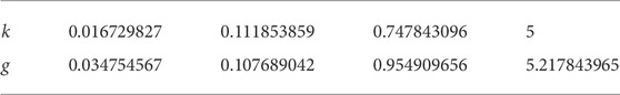
TABLE 1. Wavenumbers and weights in Ref.

4.1.2 Model validation

To validate the feasibility and accuracy of the forward modeling, an unstructured triangle method was used for forward calculations in a uniform half-space for two- and three-layer models. The resistivity of the uniform half-space was 5 Ωm, and the layered model is displayed in Figure 1. This was powered by a point source with a current intensity of 1 A, whereas k was selected as presented in Table 1. The solution obtained was compared to the theoretical value, as presented in Table 2. Evidently, the relative error between the numerical and analytical solution is small, and this validates the feasibility and accuracy of the forward modeling using the associated parameters.

FIGURE 1

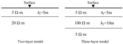
FIGURE 1. Layer model diagram.

TABLE 2

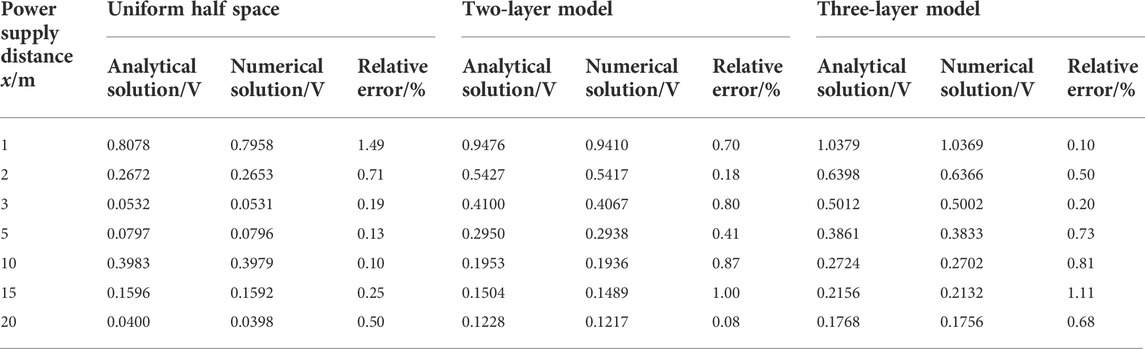
TABLE 2. Data showing a comparison of the analytical and numerical solutions for the two-dimensional geoelectric cross-section potential of the point source survey.

4.2 Forward simulation of the line source method

The expression for the uniform half-space associated with the line source method is as follows:

$U=-\int E\mathrm{d}r=-\frac{I\rho }{\pi }\int \frac{\mathrm{d}r}{r}=\frac{I\rho }{\pi }\ln \left(\frac{1}{\left|r\right|}\right)+\mathrm{c}(10)$

In this approach, the constant c depends on the position of the zero point of the reference potential. The resistivity of the uniform half space was assumed as 5 Ωm, whereas the current was 1 A, and the distance of the zero point of the potential from the power supply was 200 m. A comparison of the numerical and analytical solutions is presented in Table 3.

TABLE 3

TABLE 3. Comparison data of the analytical and numerical solutions for the uniform half-space potential of a line power source method.

According to data in Tables 2, 3, the minimum and maximum relative errors that were obtained using comsol multiphysics are 0.1% and 1.49%, respectively. These results highlight an adequate mesh, and thus, the k and g that were selected are reasonable and reliable.

5 Forward modeling

5.1 Model

As shown in Figures 2A,B, a valley and a ridge involving 45° angles were powered using both the point and line sources. The joint profile method was used for measurements, where MN = 2 m and the apparent resistivity curve is associated with a depth of 10 m, ${\rho }_1$=${\rho }_2$=${\rho }_3$=100 Ωm for Model 1. The pure terrain effect curves obtained based on the point and line sources are shown in Figures 3,4, respectively.

FIGURE 2

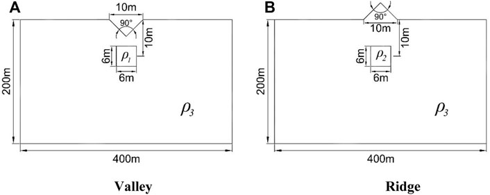
FIGURE 2. Model 1 geometry for (A) valley and (B) ridge.

FIGURE 3

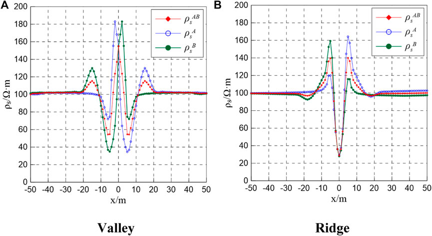
FIGURE 3. Point source pure terrain joint profile anomaly curves for (A) valley and (B) ridge.

FIGURE 4

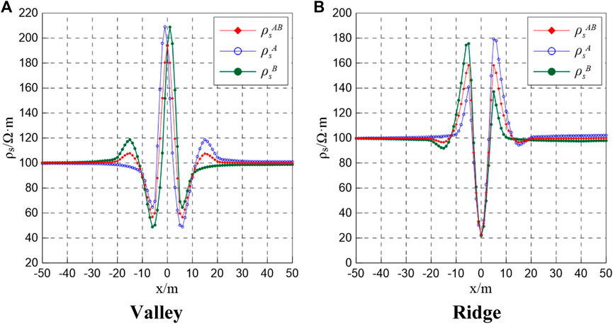
FIGURE 4. Line source pure terrain joint profile anomaly curves for (A) valley and (B) ridge.

Figures 3, 4, reveal that even though the 3D point source and 2D line source differ, the resistivity anomaly mainly occurs near the apex of the angular region. The main difference is that the terrain effect of the valley is characterized by a high-resistance anomaly, whereas that of the ridge is a low-resistance anomaly. The relative outlier can be defined using the following expression: $\epsilon =\frac{\left|{\rho }_s-{\rho }_0\right|}{{\rho }_0}$, where ρ₀ is the resistivity of the uniform half-space. The relative abnormal value of the point source is 57.32%, whereas that of the line source is 95.44%, and the terrain top effect is mainly the low resistance abnormality. The relative abnormal value of the point source is 75.12%, whereas that of the line source is 80.13%. Therefore, the line source curve is characterized by a higher variation relative to that of the point source, and this difference is probably caused by the nature of each power supply. To further explore the effect of topography on the resistivity curve, in Model 2, the following resistivity values were utilized: ρ₁ = 10 Ωm, ρ₂ = 500 Ωm, ρ₃ = 100 Ωm, Resistivity curves associated with the point and line sources are displayed in Figures 5, 6, respectively.

FIGURE 5

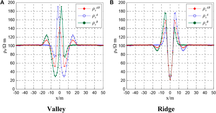
FIGURE 5. Point source joint profile anomaly curves for (A) valley and (B) ridge.

FIGURE 6

FIGURE 6. Line source joint profile anomaly curves for (A) valley and (B) ridge.

Figures 5, 6 demonstrate that because of the influence of the terrain, the low-resistance anomaly associated with the valley and high-resistance anomaly linked to the ridge cannot be accurately distinguished on the abnormal curve. At point O, a high-resistance anomaly is still present for the valley, while a low-resistance anomaly is evident for the ridge. To eliminate or minimize the influence of terrain, the comparison and the conformal transformation methods were employed to correct each anomaly curve.

5.1.1 Comparison method

The measured apparent resistivity ${\rho }_s^{\mathrm{M}}$ was divided by the corresponding pure terrain influence resistivity ${\rho }_s^{\mathrm{T}}$ to yield a corrected apparent resistivity ${\rho }_s^{\mathrm{C}}$, and this can be expressed as follows:

${\rho }_s^c=\frac{{\rho }_s^M}{{\rho }_s^T}{\rho }_{\mathrm{0}}(11)$

where ${\rho }_{\mathit{0}}$is the resistivity of surrounding rocks.

5.1.2 Coordinate network conversion method

The experimental basis was a conductive paper simulation, whereas the theoretical basis was the conformal transformation of a complex variable function. As shown in Figure 7, the topographic line in the z-plane is in the top, whereas the horizontal line in the w-plane is at the bottom. Coordinates of the w-plane can be converted into those of the z-plane using the Schwarz–Christopher transformation, which is expressed as follows:

$\frac{dz}{dw}=c{\left(w-u_1\right)}^{{\alpha }_1}(12)$

where c represents a complex constant, u₁ is the abscissa of a point on the w-plane, and α₁ is a constant that is related to the topography of the z-plane. Lines were traced upward from equidistant measurement points on the straight side to achieve the coordinate conversion and to change the position of the measuring electrode to satisfy the objective of the terrain correction.

FIGURE 7

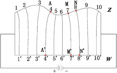
FIGURE 7. Schematic representation of the coordinate transformation.

Model (1) was used for the coordinate network conversion of the valley [Model 1 (a)]. The coordinates of the power supply point corresponding to the valley (−5, 0) are presented in Table 4.

TABLE 4

TABLE 4. Conformal transformation data corresponding to the (−5, 0) coordinate transition point.

To illustrate the problem, the valley [Model 1 (a)] was utilized for experiments. The valley-like resistivity curves in Figures 5, 6 are topographically corrected curves based on the comparison method using pure terrain curves for a valley that are shown in Figures 3, 4. Corresponding coordinates were then corrected using the conformal transformation method and the corrected apparent resistivity curve is shown in Figure 8.

FIGURE 8

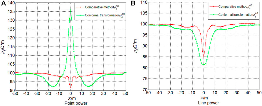
FIGURE 8. Terrain correction of the joint profile anomaly curve for a valley based on the (A) point and (B) line sources.

Evidently, the comparison method highlights adequate topographic corrections for both the point and line sources, whereas the conformal transformation exhibits suitable topographic corrections for the line source only.

Figure 9 shows a pure terrain curve of the line source that was used to correct the valley curve of the point source. Evidently, the comparison method can be exploited to use the joint profile curve of the line source to correct the terrain profile of the point source.

FIGURE 9

FIGURE 9. Line source joint profile anomaly curve correction for a valley.

6 Conclusion

DC prospecting is widely used in geophysical exploration technology The paper selects valley and ridge, and conducts 2D finite element numerical simulation of DC method through comsol multiphysics and uses comparative method and conformal transformation method for terrain correction. The main findings of the present study are summarized subsequently.

1. Profile curves of the point and line sources exhibited similar properties. Quantitative characteristics of these, however, differed. The range of variations associated with the line source was higher than that for the point source.

2. Considering that the point source involves a 3D field, whereas the line source is associated with a 2D field, the results showed that the former was unsuitable for terrain correction based on the conformal transformation. The point and line sources are both suitable for terrain correction according to the comparison method.

3. Even though fields of the point and line sources differ, the joint profile curve of the line source was still suitable for correction of the joint profile curve of the point source.

The selection of wavenumbers failed to yield universality. Therefore, further research is required on this aspect to enhance practical application of the approach presented for terrain corrections.

Data availability statement

The original contributions presented in the study are included in the article/Supplementary Material, further inquiries can be directed to the corresponding author.

Author contributions

HX: Methodology, data analysis and writing. LL: Data analysis, model. ZL: Data analysis, model calculation. JL: Reviewing and editing, drawing. GL: Article review and concept of the article. WL: Article review and concept of the article.

Conflict of interest

ZL and JL were empolyed by Xi’an Research Institute China Coal Technology & Engineering Group Corp, Shaanxi Coal Chemical Industry Technology Research Institute Co., Ltd.

The remaining authors declare that the research was conducted in the absence of any commercial or financial relationships that could be construed as a potential conflict of interest.

Publisher’s note

All claims expressed in this article are solely those of the authors and do not necessarily represent those of their affiliated organizations, or those of the publisher, the editors and the reviewers. Any product that may be evaluated in this article, or claim that may be made by its manufacturer, is not guaranteed or endorsed by the publisher.

References

Afanasenkov, A. P., and Yakovlev, D. V. (2018). Application of electrical prospecting methods to petroleum exploration on the northern margin of the Siberian Platform. Russ. Geol. Geophys. 59 (7), 827–845. doi:10.1016/j.rgg.2018.07.008

CrossRef Full Text | Google Scholar

Chen, M., and Yan, Y. (1987). Finite element forward calculation of apparent resistivity of two-dimensional horizontal electric dipole frequency conversion sounding impedance. J. Geophys. 2, 201–208.

Google Scholar

Cheng, J., Li, F., Peng, S., and Sun, X. Y. (2014). Research progress and prospect of advance detection of geophysical methods in mine roadway. J. China Coal Soc. 39 (08), 1742–1750. doi:10.13225/j.cnki.jccs.2014.9007

CrossRef Full Text | Google Scholar

Cui, S., Pei, X., Jiang, Y., Wang, G., Fan, X., Yang, Q., et al. (2021). Liquefaction within a bedding fault: Understanding the initiation and movement of the Daguangbao landslide triggered by the 2008 Wenchuan Earthquake (Ms = 8.0). Eng. Geol. 295, 106455. doi:10.1016/j.enggeo.2021.106455

CrossRef Full Text | Google Scholar

Dhu, T., and Graham, H. (2004). Numerical and laboratory investigations of electrical resistance tomography for environmental monitoring. Explor. Geophys. 35 (1), 33–40. doi:10.1071/eg04033

CrossRef Full Text | Google Scholar

He, J., and Zhou, Z. (1975). Problems of point power field and line power field in resistivity topography correction. Geol. Explor. 8, 45–51.

Google Scholar

Ji, Y., Huang, T., Huang, W., Li, T. L., and Wang, Y. (2016). 2D anisotropic magnetotelluric numerical simulation using meshfree method under undulating terrain[J]. Chin. J. Geophys. 59 (12), 4483–4493. doi:10.6038/cjg20161211

CrossRef Full Text | Google Scholar

Jin, C., and Liu, J. (2014). Two-dimensional numerical simulation and application of the high-density resistivity method. Geol. Explor. 50 (5), 0984–0990. doi:10.13712/j.cnki.dzykt.2014.05.019

CrossRef Full Text | Google Scholar

Kaznacheev, P. A., Popov, I. Y., Modin, I. N., and Zhostkov, R. A. (2020). Application of independent finite element modeling for estimating the effect of simplest landforms on results of inversion of electrical resistivity tomography data (example of a trench with the triangular cross-section). Seism. Instr. 56 (5), 531–539. doi:10.3103/s0747923920050084

CrossRef Full Text | Google Scholar

Kumar, S., Patro, P. K., and Chaudhary, B. S. (2018). Three dimensional topography correction applied to magnetotelluric data from Sikkim Himalayas. Phys. Earth Planet. Interiors 279, 33–46. doi:10.1016/j.pepi.2018.04.001

CrossRef Full Text | Google Scholar

Li, H., Deng, J., Feng, P., Pu, C., Arachchige, D., and Cheng, Q. (2021). Short-term nacelle orientation forecasting using bilinear transformation and ICEEMDAN framework. Front. Energy Res. 9, 780928. doi:10.3389/fenrg.2021.780928

CrossRef Full Text | Google Scholar

Li, H., Deng, J., Yuan, S., Feng, P., and Arachchige, D. (2021). Monitoring and identifying wind turbine generator bearing faults using deep belief network and EWMA control charts. Front. Energy Res. 9, 799039. doi:10.3389/fenrg.2021.799039

CrossRef Full Text | Google Scholar

Li, H., He, Y., Xu, Q., Deng, J., Li, W., and Wei, Y. (2022). Detection and segmentation of loess landslides via satellite images: A two-phase framework. Landslides 19, 673–686. doi:10.1007/s10346-021-01789-0

CrossRef Full Text | Google Scholar

Li, H. (2022). SCADA data based wind power interval prediction using LUBE-based deep residual networks. Front. Energy Res. 10, 920837. doi:10.3389/fenrg.2022.920837

CrossRef Full Text | Google Scholar

Li, H. (2022). Short-term wind power prediction via spatial temporal analysis and deep residual networks. Front. Energy Res. 10, 920407. doi:10.3389/fenrg.2022.920407

CrossRef Full Text | Google Scholar

Lu, X., Zhang, S., and Cui, X. (2014). Finite element forward modeling of 2.5 dimensional resistivity based on anomalous field. Geophys. Prog. 29 (6), 2718–2722. doi:10.6038/pg20140637

CrossRef Full Text | Google Scholar

Ma, C., Liu, J., Guo, R., Liu, R., Ciu, Y., Liu, R., et al. (2018). Element-free Galerkin forward modeling of DC resistivity using a coupled finite element method with extended the boundaries. Geophys 61 (06), 2578–2588. doi:10.6038/cjg2018L0492

CrossRef Full Text | Google Scholar

Ma, C., Liu, J., Liu, H., Guo, R., Bello, M., and Cui, Y. (2019). 2.5D electric resistivity forward modeling with element-free Galerkin method. J. Appl. Geophys. 162, 47–57. doi:10.1016/j.jappgeo.2018.12.021

CrossRef Full Text | Google Scholar

McCubbine, J. C., Featherstone, W. E., and Kirby, J. F. (2017). Fast-Fourier-based error propagation for the gravimetric terrain correction. Geophysics 82 (4), G71–G76. doi:10.1190/geo2016-0627.1

CrossRef Full Text | Google Scholar

Peng, Y., Liu, J., Liu, H., and Tang, J. (2014). Numerical simulation of dc resistivity 2.5 dimensional finite element. Geophys. Prog. 29 (4), 1926–1931. doi:10.6038/pg20140461

CrossRef Full Text | Google Scholar

Ren, Z., Qiu, L., Tang, J., Feng, Z., Chen, C. J., Chen, H., et al. (2018). 3D modeling of direct-current anisotropic resistivity using the adaptive finite- element method based on continuity of current density. Geophys. J. 61 (01), 331–343. doi:10.6038/cjg2018K0698

CrossRef Full Text | Google Scholar

Saber, J., Mohammad, P., and Kamal, K. (2020). High accuracy gravity terrain correction by optimally selecting sectors algorithm based on Hammer charts method. Studia Geophysica et Geodaetica 64 (prepublish). doi:10.1007/s11200-019-0273-0

CrossRef Full Text | Google Scholar

Sola, I., González-Audícana, M., and Álvarez-Mozos, J. (2016). Multi-criteria evaluation of topographic correction methods. Remote Sensing of Environment. 184, 247–262. doi:10.1016/j.rse.2016.07.002

CrossRef Full Text | Google Scholar

Song, W., Wang, Y., and Shao, Z. (2016). Numerical simulation of coal field fire area by high density electrical method and magnetic method. J. China Coal Soc. 41 (04), 899–908. doi:10.13225/j.cnki.jccs.2015.0871

CrossRef Full Text | Google Scholar

Tang, J., Wang, F., and Ren, Z. (2010). 2.5-d dc resistivity adaptive finite element numerical simulation based on unstructured grid. J. Geophys. 53 (03), 708–716. doi:10.3969/j.issn.0001-5733.2010.03.02

CrossRef Full Text | Google Scholar

Valera Sifontes, R, and Sato, H K (2019). Relief effects correction on frequency-domain electromagnetic data. Geophysics 84 (1), E11. doi:10.1190/geo2017-0452.1

CrossRef Full Text | Google Scholar

Wang, J., and Geng, Y. (2015). Terrain correction in the gradient calculation of spontaneous potential data. Chin. J. Geophys. 58 (6), 654–664. doi:10.1002/cjg2.20202

CrossRef Full Text | Google Scholar

Wang, X., Feng, H., and Tian, H. (2011). Direct current forward modeling based on Comsol Multiphysics. Coal Geol. Explor. 39 (5), 76–80. doi:10.3969/j.issn.1001-1986.2011.05.019

CrossRef Full Text | Google Scholar

Xie, H., Li, Z., and Li, S. (2019). Finite element 2D forward modeling of DC method with line source. Coal field Geol. Explor. 47 (01), 194–199. doi:10.3969/j.issn.1001-1986.2019.01.030

CrossRef Full Text | Google Scholar

Xu, S., and Lou, Y. (1987). Boundary element method of two-dimensional field extension and conversion of undulating terrain. Geophys. Geochem. Explor. Comput. Technol. 3, 195–199.

Google Scholar

Xue, G., Chang, J., and Lei, K. (2021). Review on three-dimensional simulations of transient electromagnetic field. J. Earth Sciences Environ. 43 (03), 559–567. doi:10.19814/j.jese.2020.11029

CrossRef Full Text | Google Scholar

Xue, G., Yan, S., and Chen, W. (2016). A fast topographic correction method for electromagnetic data. J. Geophys. 59 (12), 4408–4413. doi:10.6038/cjg20161202

CrossRef Full Text | Google Scholar

Yang, H., and Li, J. (1999). Numerical simulation of the influence of undulating topography on the charging law of surrounding rock in close mines. Geophys. Geochem. Explor. 3, 43–51+56.

Google Scholar

Zhang, J., Zhi, Q., and Li, X. (2013). 2.5D finite element numerical simulation for electric dipole source on ridge terrain. Chin. J. Nonferrous Metals 23 (9), 2540–2550. doi:10.19476/j.ysxb.1004.0609.2013.09.025

CrossRef Full Text | Google Scholar

Zhang, M., Colin, G. F., and Liu, C. (2021). 2.5-D forward modeling of the electromagnetic response in frequency-domain ground-airborne areas with topographic relief. J. Geophys. 64 (01), 327–342. doi:10.6038/cjg2020N0182

CrossRef Full Text | Google Scholar

Zhang, Q., Dai, S., and Chen, L. (2016). DC resistivity method under the condition of multi-source an approximate boundary conditions in finite element three-dimensional numerical simulation. J. Geophys. 59 (9), 3448–3458. doi:10.6038/cjg20160927

CrossRef Full Text | Google Scholar

Zhang, Y., Wang, G., Li, H., Lian, Y., Li, W., Qiu, H., et al. (2021). Efficient 3D vector finite element modeling for TEM based on absorbing boundary condition. J. Geophys. 64 (03), 1106–1118. doi:10.6038/cjg2021N0137

CrossRef Full Text | Google Scholar

Zhou, J., Wei, J., Yang, T., Zhang, P., Liu, F., and Chen, J. (2021). Seepage channel development in the crown pillar: Insights from induced microseismicity. Int. J. Rock Mech. Min. Sci 145, 104851. doi:10.1016/j.ijrmms.2021.104851

CrossRef Full Text | Google Scholar

Zhu, J. (2022). Three-dimensional Electromagnetic modeling using spectral element method with tetrahedral grid [D]. Jilin University. doi:10.27162/d.cnki.gjlin.2022.000584 (in Chinese)

CrossRef Full Text | Google Scholar

Zhu, J., Yin, C., Liu, Y., Liu, L., Yang, Z., Qiu, C., et al. (2020). 3-D dc resistivity modelling based on spectral element method with unstructured tetrahedral grids. Geophys. J. Int. 220 (3), 1748–1761. doi:10.1093/gji/ggz534

CrossRef Full Text | Google Scholar