 Wei Zhang
 Jianyun Gao
 Qiaozhen Lai
 Yanzhen Chi
 Tonghua Su
- 1Fujian Key Laboratory of Severe Weather, CMA, Fuzhou, China
- 2State Key Laboratory of Severe Weather, Chinese Academy of Meteorological Sciences, Beijing, China
- 3Longyan Meteorological Bureau, Longyan, China
- 4Xiamen Meteorological Bureau, Xiamen, China
- 5Fujian Climate Center, Fuzhou, China
Several probabilistic forecast methods for heatwave (HW) in extended-range scales over China are constructed using four models (ECMWF, CMA, UKMO, and NCEP) from the Subseasonal-to-Seasonal (S2S) database. The methods include four single-model ensembles (SME; ECMWF, CMA, UKMO, and NCEP), multi-model ensemble (MME), and Bayesian model averaging (BMA). The construction and verification of reforecasts are implemented by a defined heat wave index (HWI) which is not only able to reflect the actual occurrence of heatwaves, but also to facilitate forecast and verification. The performance is measured by traditional verification method at each grid point of the 105°E to 132°E; 20°N to 45°N domain for the July, August, and September (JAS) of 1999–2010. For deterministic evaluations of HWI forecast, BMA shows a better pattern correlation coefficient than SME and MME and comparable equitable threat score (ETS) with ECMWF and MME. The good performance of ECMWF and MME take advantage of setting the percentile thresholds for forecasting HW. For the probabilistic forecast, the Brier score of BMA is comparable (superior) to that of MME and ECMWF at short (long) lead-time. BMA also demonstrates an improvement on the reliability of probabilistic forecast, indicating that BMA method is a useful tool for an extended-range forecast of HW. Meanwhile, in the real-time extended-range probabilistic forecast, the beginning date, end date, and probability of HW event can be predicted by the HWI probabilistic forecast of BMA.
1 Introduction
The heat wave (HW) is one of the extreme events around the world. It causes widespread destruction of infrastructure and human activity, economic damage, and loss of life. It is well known that the frequency and intensity of HWs are remarkably increased in the past years around various parts of the world due to climate change. Typical HW events of recent years are central Europe in 2003 (Fink et al., 2004; Fouillet et al., 2006; Schär et al., 2004; Trigo et al., 2005), over Russia in 2010 (Barriopedro et al., 2011; Dole et al., 2011), and over Europe in 2018 (Schiermeier, 2018). The 2010 Russian HW was the strongest recorded over the past 30 years (Hoag, 2014). It caused about 55,000 deaths and numerous wildfires, the worst drought in Russia in nearly 40 years, and the loss of at least millions of hectares of crops. Moreover, in the past summer (late June 2021), the Pacific North-West HW crossing the US and Canada has been called a roughly 1-in-1,000-years event (www.climate.gov 2021: https://www.climate.gov/news-features/event-tracker/preliminary-analysis-concludes-pacific-northwest-heat-wave-was-1000-year). In East China, the temperature has increased significantly in the past 50 years, and the HW is one of the major disastrous weathers in this region (Shi et al., 2008). In summer 2013, this region experienced its worst HW on record for the past 113 years (Xia et al., 2016). The time needed to prepare for a persistent extreme event is often beyond the skillful prediction timescales of a few days that are currently available (White and Coauthors, 2017). Demands are growing rapidly in the operational prediction and applications communities for forecasts that fill the gap between medium-range weather and long-range or seasonal forecasts, and the extended-range forecast. However, it has been less well addressed despite the considerable socio-economic value that could be derived from such forecasts.
The establishment of an extensive database (Vitart et al., 2017), containing sub-seasonal (up to 60 days) forecasts by the WMO S2S research demonstration project makes the forecasting of HW in this time range possible. However, the accuracy of the extended range forecast is limited due to the chaotic characteristics of the atmosphere and uncertainties associated with initial conditions and models (Thompson, 1957; Lorenz, 1963, 1969; Smagorinsky, 1969). Probabilistic forecasts are becoming an inevitable method of solving this problem (Carrol and Maloney, 2004). Probabilistic forecasts aim to predict the uncertainty of a quantity or event of interest in the form of full predictive probability distributions (Gneiting and Katzfuss, 2014) rather than single-valued or point forecasts. Information about the uncertainty of a forecast can provide decision-makers with a range of possible outcomes and the amount of confidence associated with a particular event (Krzysztofowicz, 2001), which is valuable for deciding if, when, and how many precautionary measures should be taken. Besides, the use of probabilistic forecasts can realize more economic value than control forecasts for most potential users according to cost-loss ratios (Zhu et al., 2002). Especially at and beyond 120 h lead-time, all users are better off using the ensemble system than the control forecasts. Therefore, we focus this paper on the generation and validation of probabilistic forecasts for heatwaves in the extended range.
Several methods are currently used to construct probabilistic forecasts from the ensemble forecast. The probability of a single model ensemble (SME) is derived by computing the ratio of ensemble members with events that occur to all members. For this probabilistic forecast to be accurate and reliable, it is necessary to enlarge ensembles, which represent a range of possible evolutions of the system given the uncertainties (Richardson, 2000). In addition, modeling uncertainties can be taken into account by combining ensemble forecasts from several models and forming a multimodel ensemble (MME; Krishnamurti, 1999). Even still, raw ensemble (SME and MME) forecasts do not capture the full range of forecast scenarios and bear uncertainties that grow larger as lead time increases (Hamill and Colucci 1997; Raftery et al., 2005; Stauffer et al., 2017). Bayesian model averaging (BMA; Raftery et al., 2005; Sloughter et al., 2007, 2010; Fraley et al., 2010) is one of the state-of-the-art approaches developed for ensemble-based probabilistic precipitation forecasts. The BMA predictive probability density function (PDF) is a weighted average of PDFs centered on the individual bias-corrected forecasts, where the weights are equal to posterior probabilities of the models generating BMA model and reflect the models’ relative contributions to predictive skill over the training period (Raftery et al., 2005). It was originally applied to the prediction of temperature and sea level pressure, and those PDFs were approximately normal distribution, yielding well-calibrated and sharp PDFs. Many analyses demonstrated that the BMA method performed superior to raw ensemble forecasts (Sloughter et al., 2007; Schmeits and Kok 2010; Liu and Xie, 2014). Subsequently, the method was employed in more studies (Casanova and Ahrens 2009; Erickson et al., 2012; Liu and Xie, 2014) for the short- and medium-range forecasts with TIGGE (The THORPEX Interactive Grand Global Ensemble) dataset. However, it is unclear whether BMA is fit for the probabilistic forecast of heatwave and whether it performs better than raw ensembles in the S2S time scale. In this framework, we seek to answer this question by constructing probabilistic reforecasts of SME, MME, and BMA for heatwave and evaluating these reforecasts skills, specifically probabilistic skill, based on a S2S dataset.
Since a heatwave is an event with consecutive hot days in one region and daily maximum surface temperatures is not enough to represent it, it is necessary to develop an index based on daily maximum surface temperatures that not only reflects the actual occurrence of heatwaves but also facilitates probabilistic forecast and verification. The heatwave has been widely identified by an extreme heat factor (EHF) index based sliding 3-days window of temperature (Nairn et al., 2009). But this index does not apply to this study because it is difficult for this discontinuous variable to construct proper PDFs. Another type of heatwave is defined as one pentad mean surface maximum air temperatures exceeding the local 95th percentiles during the control period of 1960–1990 (Zhu and Li, 2017). The defects of this definition, which does not consider the continuity of the heatwave, also make it unavailable to this study. Fischer and Schär (2010) defined a heatwave as a spell of at least six consecutive days with maximum temperatures exceeding the local 95th percentile over a control period. This heatwave is based on the synoptic temperatures, which will not engage any extended-range skill. How to synthesize the aforementioned points and then develop a skillful HWI in the extended range is another major topic in this study.
The metrics applied to verify the hindcasts, and the data used are described in Section 2. The definitions of HWI and heatwave are described in Section 3, which also shows the construction of a probabilistic reforecast for HWI. The forecasting skills for the different reforecasts are compared in Section 4. Section 5 summarizes the results and discusses the real-time probabilistic prediction of heatwaves based on HWI.
2 Data and Verification Methods
2.1 Data
The S2S database (Vitart et al., 2017) collects forecasts/reforecasts (or hindcasts) from the subseasonal forecasting systems of 11 different centers. The individual systems, including the China Meteorological Administration (CMA), the European Center for Medium-range Weather Forecast (ECMWF), the National Centers for Environmental Prediction (NCEP), and the United Kingdom Met Office (UKMO) are selected as SME. The configuration details of the four systems are summarized in Table 1. The daily maximum temperature has been extracted from the four different reforecast systems for the common 12-years (1999–2010) summertime (July to September). Given that all atmospheric models have different native horizontal and vertical resolutions, the S2S data are extracted on a common 1.5 × 1.5° grid on the China domain (105°E to 132°E; 20°N to 45°N). The constructions of MME and BMA require the same initial dates for all four systems. The different reforecast frequencies shown in Table 1 could be a challenge to build. Here we chose to overcome this drawback by selecting the calendar dates of the ECMWF reforecast as the referred starting dates, with others corresponding to these dates. It is easy for the daily CMA and NCEP to complete this correspondence. For UKMO, the closest date (early or later) is selected to construct MME and BMA, which means that there may exist different forecasting valid in MME and BMA. Nevertheless, the operation will not create an issue with the extended range forecast.
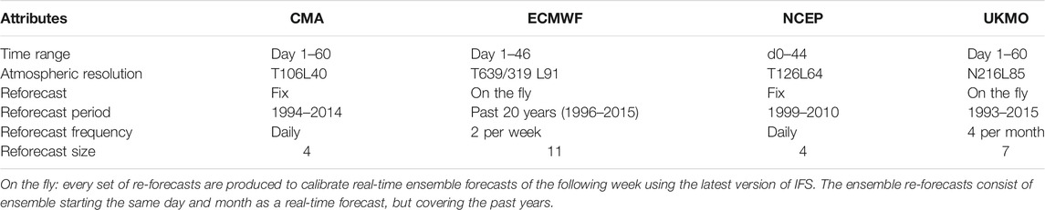
TABLE 1. Reforecast attributes for the four systems from the WMO S2S database.
The observed daily maximum temperatures of 2,248 stations in China are provided from the Chinese Meteorological Information Center. The station data are interpolated onto the common 1.5° × 1.5° grid to match up the forecasts in the S2S database by natural neighbor interpolation method and used to BMA train and verification for reforecasts over 1999–2010.
2.2 Verification Methods
2.2.1 Mean Absolute Error and Pattern Correlation Coefficient
The mean absolute error (MAE) and pattern correlation coefficient (PCC) are defined by
where
2.2.2 Equitable Threat Score
The ETS represents the deterministic forecasting skill of heatwaves and is specified as follows:
Variables in the formula are defined in Table 2. ETS takes a random chance [R(a)] away to account for true forecast skill. Larger ETS values represent higher forecasting skills, while ETS less than 0 donates no skill in the forecast.
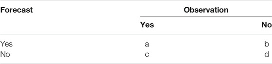
TABLE 2. Heatwave test classification.
The probability of detection (POD), false-alarm rate (FAR), and miss rate (MSR) are also employed to assess the deterministic forecast as follows:
2.2.3 Brier Score
The Brier score has been widely used in the assessment of probabilistic forecasts (Ferro 2007). It is essentially the mean-squared error of the probability forecasts, considering that the observation
Where n is the number of forecast/event pairs, i denotes a numbering of the n and
2.2.4 Brier Skill Score
The Brier skill score (BSS) is:
Where
Ideally, the climatological probabilities would be determined from independent data, but commonly they are calculated from the sample observed data. In the conventional method of calculation, an average climatology
Considering the differences between the climatological event frequencies for different months, the sample
2.2.5 Continuous Ranked Probability Score
The CRPS measures the difference between the predicted and occurred cumulative distributions
Where
3 Heat Wave Index and its Probabilistic Forecast
3.1 HWI and Heat Waves
In this study, we define HWI as a sliding 5-days window and 9-points equal weight average of the daily surface maximum temperatures. For each grid point, a heatwave is a period with HWI continuously greater than a certain percentile threshold. The percentile is referred to the ratio of daily surface maximum air temperatures below 35
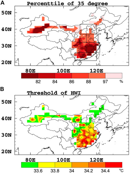
FIGURE 1. (A) The percentiles of greater and equal to 35
The HWI is developed from the points of definitions of heatwave in previous studies (Nairn et al., 2009; Fischer and Schär, 2010; Perkins eta al., 2012; Zhu and Li., 2017) and for facilitation of probabilistic forecast and verification. First, the 5-days running average referred to Nairn et al. (2009), has filtered the synoptic and small-scale noise that it can represent the large-scale and long-lasting weather event to enhance extended-range forecast capability (Buizza and Leutbecher, 2015). The spatial running average is implemented to match the time running average coordinately representing equivalence scales. Second, the running average of daily temperature may also match normal distributions that HWI may be fitted to use BMA. A previous study (Raftery et al., 2005) has proved that predictive PDFs of BMA were much better calibrated than the raw ensemble. Whether the PDF of HWI fits normal distributions will be examined in the following section. Third, the daily HWI will be facilitated for verification when using the traditional verification method mentioned above.
The observed HWI is mainly defined to consider the key properties addressed through its extreme and persistence in terms of the period and surrounding area. The extreme property of the HWI is seen from the value of percentile (Figure 1A) ranging from 80 to 92. The average persistent days of the observed heat wave identified by HWI being greater than 5 days (Figure 2A) indicates persistent property.
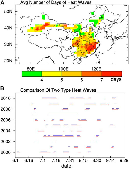
FIGURE 2. (A) The number of average persistent days of the observed heat wave identified by HWI, and (B) comparison for the period of heatwaves in this study (red line) and in Lin et al. (2021) (blue line) over Huanan from 2000 to 2010 (B).
To further examine whether heatwaves determined by HWI are objective, we compare them with the heatwaves in Lin et al. (2021). Based on observation data from weather stations, they objectively define the heat waves in four regions of China (the four boxes in Figure 1A) by considering the certain percentage of stations with a maximum temperature greater than 35°C, the coincidence degree of stations comparing with the previous day, and the persistent days (See Lin et all., 2020 for more details). For comparison, we reconstruct HWI by four regional averages instead of the spatial running average. The corresponding thresholds are calculated by the four regional averages of percentiles in Figure 1A, which are 0.82, 0.80, 0.93, and 0.97 respectively. Basing the reconstructed HWI and threshold, we obtained the four regional heatwaves of our study. We found that 90 percent of these events are consistent with the heat waves in Lin et al. (2021).
Figure 2B shows the period of these two types of heatwave that occurred from 2000 to 2010 in South China. The result indicates great consistency, verified the rationality of our definition for HWI.
3.2 Single- and Multi-Model Ensemble Probabilistic Forecast of HWI
For short- and medium-range forecasts the extreme threshold are generally defined from observations or reanalysis and are often replaced by fixed boundaries that have societal implications. However, numerical models drift with increasing lead-time very quickly toward their own climate, which can be very different from observations. Therefore, for extended-range forecasts, the preferred option is to define the percentile thresholds from reforecasts (Vitart and Robertson, 2018). The reforecasts of HWI for SME and MME are obtained by sliding 5-days window and 9-points running average on the ensembles of SME and MME respectively. Then based on the ensemble means of reforecast and the percentile shown in Figure 1A, the thresholds of different ensembles and different forecast validations (Figure 3) are calculated. Finally, the probabilistic forecast of heatwave for each SME and MME will be obtained by calculating the percentage of members with HWI greater than the corresponding threshold.
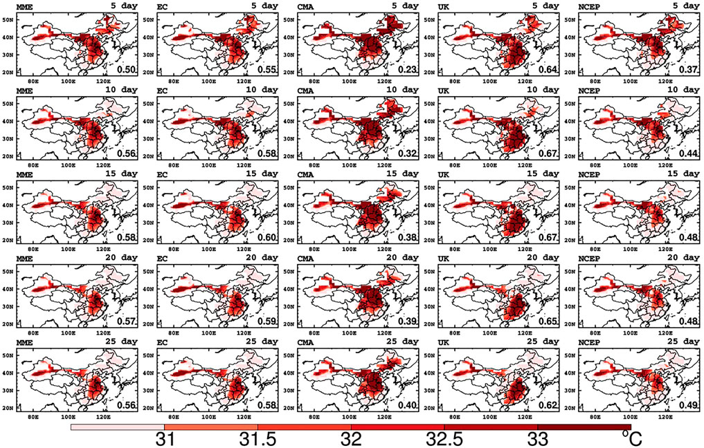
FIGURE 3. The thresholds (°C) of HWI for MME, EC, CMA, UK, NCEP (columns from left to right) forecasts from the different forecasting valid days (5-, 10-, 15-, 20-, 25-days; rows from top to bottom). The digits in the lower right corner of each panel are the correlation of this pattern with the observational threshold pattern.
Figure 3 shows that the value of the threshold varies among different ensembles and different forecast validations. The threshold of each ensemble shows a decreasing trend with the forecast timeliness, indicating that the numerical models quickly drift toward their own climatology. So, it is necessary to set a threshold along with forecast time. In terms of overall intensity and location, the threshold of the United Kingdom is closest to the observation, indicating that the HWI climatological distribution of the United Kingdom matches the observation best. This view can be visually proved by the largest correlation of the United Kingdom threshold with the observational threshold (digital in the lower right corner of each panel in Figure 3). The results implied that the United Kingdom may perform a higher forecast skill in HWI forecast. Although the threshold of CMA is the largest among SMEs, MME and its magnitude are closest with the threshold of observation (Figure 1B), the center of the large values has shifted to the north.
The definition of HWI and the forecasting thresholds for SMEs and MME make the extended-range forecast of heatwave events possible. As shown in Figure 4, the ETS of ECMWF for HWI (green line) reaches up to 0.3 in the first 10-days forecast and maintain greater 0.2 in the 10–30-days forecast, while the ETS of daily maximum air temperature for 35°C (blue line) is less than 0.2 during the 1–30-days forecast. This contrast shows that the daily maximum temperature and fixed thresholds are not fit for extended-range prediction of HW events. It is necessary to define the HWI and set its forecasting thresholds for SMEs and MME. Besides, the better forecasting skill of the HWI (green line) than the 5-days running average of daily maximum temperature (red line) proves the necessity of spatial average in the definition of HWI.
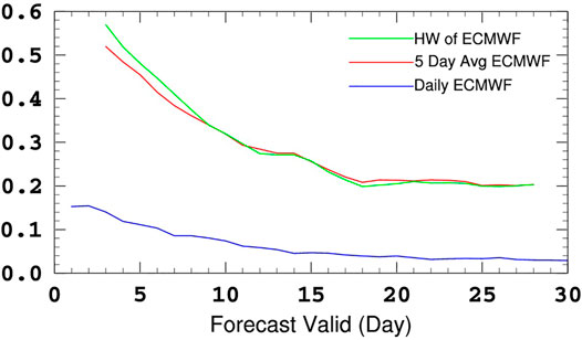
FIGURE 4. The ETS of ECMWF for daily maximum air temperature greater than 35°C (blue line), 5-days running average of daily maximum temperature (red line), and HWI (green line) greater than their relative thresholds.
3.3 Bayesian Model Averaging Probabilistic Forecast of HWI
The BMA model used in this study followed Raftery et al. (2005) and is only briefly described here. The BMA method generates a total PDF of HWI amount by weighted averaging PDFs estimated from bias-corrected forecasts of individual ensemble members, which is defined as
where y is the HWI quantity, f is the forecast of a particular ensemble member, k is the index of the ensemble member, K is the total number of the ensemble members,
The poor POD, MSR, FAR, and ETS of raw ensemble members for heatwave events (dash line in Figure 5) shows the bias-corrected requirement for each ensemble before doing BMA. In our study, linear regression is applied to correct bias for each SMEs. The parameters are obtained by training with some observation/forecast pairs. It is indicated that bias correction has significantly improved the forecasting skill of ECMWF (solid line in Figure 5). The bias-corrected forecasts of the individual ensemble will contribute to the forecasting capability of BMA.
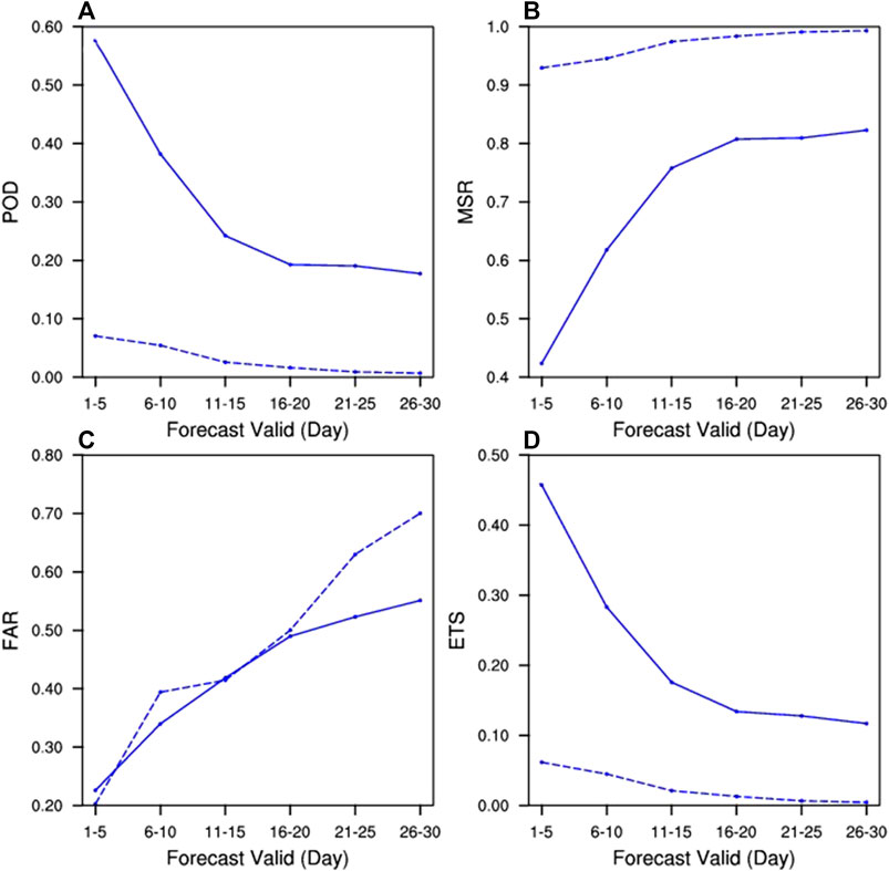
FIGURE 5. Comparison of the raw (dash lines) and bias-corrected (solid lines) ECMWF forecast for POD (A), MSR (B), FAR (C), and ETS (D) of heatwave events.
The BMA was developed initially for quantities whose PDFs can be approximated by normal distributions, such as temperature and sea level pressure. Whether normal distribution fit the PDF of HWI is necessary to be examined. As we are mainly concerned with the probabilistic forecast of heatwaves, only the distributions of observed HWI conditional on forecasting heatwaves are shown in Figure 6 for different lead times and ensembles. It is shown that the normal distribution fits HWI for all of them. Especially, the distribution of EC is better approximated by normal shape than other SMEs as its value varies more smoothly.
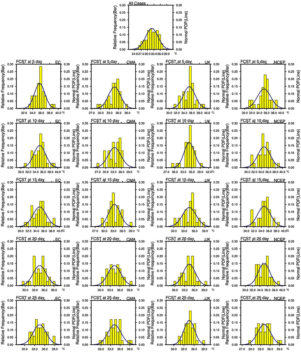
FIGURE 6. Histograms of observed HWI conditional on the forecasting of heatwaves. The rows from top to bottom correspond to the lead days at 5, 10, 15, 20, 25. The columns from left to right correspond to the different forecast models (ECMWF, CMA, UKMO, NCEP).
On the basis of the normal distribution of HWI, the following steps can finish the training of BMA. The conditional PDF by a normal distribution is centered at a linear function of the forecast,
In our implementation, the training set consists of a sliding window of forecasts and observations for the previous m samples, where m = 7,12, 17, 22.27. The certain number of samples when the verification metrics tend to be stable is taken as the optimal sliding training number. Here we adopt the mean absolute error (MAE) and continuous rank probabilistic score (CRPS) as the verification metrics. As shown in Figure 7, the short-term forecasts (blue lines and green lines in Figure 7) require about 12 training samples to have the best MAE and CRPS scores. But for long-term forecasts (yellow lines and red lines in Figure 7), 20 samples obtains the best probabilistic forecast skill with optimal CRPS score (Figure 7B). Since this article focuses on the probabilistic forecasting of the extended period, 20 sliding samples are selected for BMA model training. Figure 7C shows the average weights of each ensemble trained from BMA when using 20 sliding samples. BMA automatically adjusts the weights for each ensemble according to their performance during the training period so that BMA may engage a better forecasting skill than SMEs and MME.
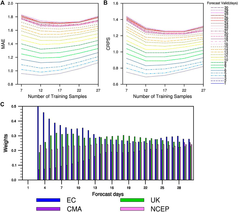
FIGURE 7. The MAE (A) and CRPS (B) of BMA as a function of the number of samples used for BMA training. The different patterns of lines indicate different forecast valid days. The average weights (C) of four individual ensemble members were used for BMA when using 20 sliding samples.
The definition of the threshold for HWI of BMA is similar to SMS and MMS, which is based on the percentile from reforecasts (Figure not shown). According to the PDF and threshold for HWI of BMA, a probabilistic forecast of BMA for heatwave is obtained.
4 Verification for Heatwaves
Seeking the continuous days with HWI greater than extreme percentile thresholds respectively can identify the observed and forecast heat waves. But it is not easy to quantitatively verify the forecasting heatwaves against observed heatwaves. Some of the investigations only verify the forecast skill of heatwave qualitatively on the case studies (Hudson et al., 2016; Mandal et al., 2019). To solve this problem, the daily forecasting HWI is verified against daily-observed HWI using the traditional verification method. It implied that the verification of heatwaves is executed by decomposing these events into individual days. These deterministic and probabilistic reforecasts of SME, MME, and BMA are verified for the 1999–2010 JAS period at each grid point of the domain.
4.1 Deterministic Verification for Heatwaves
The PCC, POD, MSR, FAR, and ETS are used to evaluate each deterministic HWI reforecasts that is the ensemble mean of their members for SMS and EMS. The PCC shown in Figure 8 indicates that the HWI of BMA possesses the best pattern correlation to observed HWI with a coefficient up to 0.92. Though the PCC of BMA decreases with lead time, its value is still over 0.8 in the extended range. For SMS and EMS, the UK displays the best pattern correlation with observation, which is consistent with the rank of the spatial correspondence between the threshold of ensembles (Figure 3) and observation (Figure 1B). The POD, MSR, FAR, and ETS scores for heatwave forecasts are presented in Figure 9. ETS skills of BMA, ECMWF, and MME are the best among all reforecasts and are comparable across themself for all lead times. The POD, MSR, and FAR show consistent skill with ETS. The CMA performs the worst among all forecasts for all scores. Given this, we have tried to improve the BMA without CMA, based on ECMWF, UK, and NCEP. The performance of BMA based on three models is almost the same as BMA based on four models. Therefore, BMA based on four models is adopted in this paper.
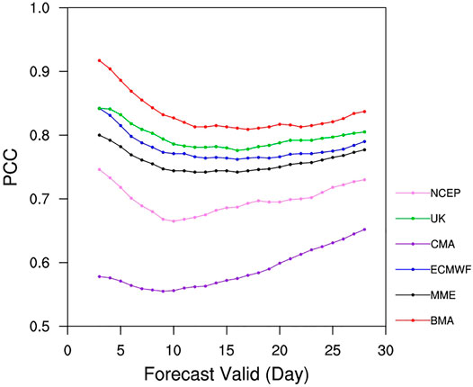
FIGURE 8. Pattern correlation of the daily PHEI between the observed dataset and different model forecasts as a function of forecast lead days.
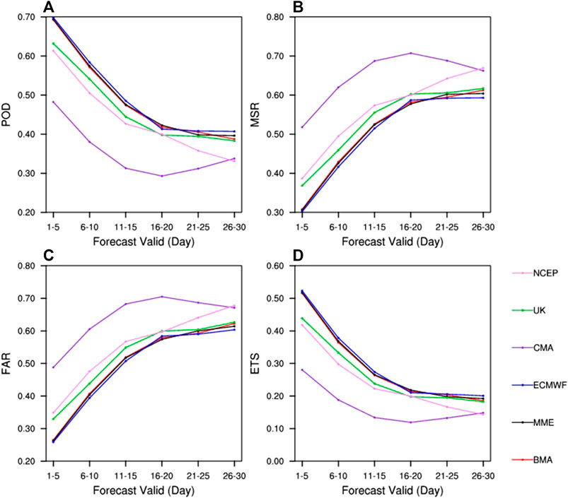
FIGURE 9. The POD (A), MSR (B), FAR (C), and ETS (D) as a function of forecast lead days for different reforecasts of heatwaves.
4.2 Probabilistic Verification for Heatwaves
The probabilistic performance for heatwave of BMA is compared to the MMEs and SME for the JAS start dates of the common period 1999–2010. The BS, reliability, and BSS are employed to verify the performance. Since our study focused on the dichotomous extreme events and CRPS measures the overall probabilistic performance, it is not employed here. BS is used in the assessment of probabilistic forecasts of events exceeding extreme thresholds, which are set separately for observation and forecast. Figure 10 shows the BS score at each lead day for heatwave forecast of BMA, SMSs, and MMS. As it shows, the performance of BMA is comparable (superior) to that of MME and ECMWF at small (large) lead times. The result suggests that the BMA model, based HWI, is fit for the probabilistic forecast of heatwaves in the S2S time scale.
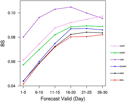
FIGURE 10. The BS for heatwave as a function of forecast lead days for different reforecasts including SMEs, MME, and BMA.
As pointed out by Murphy (1973), the algebraic decomposition of the Brier score is expressed as three terms, reliability, resolution, and uncertainty. According to the research of Weisheimer and Palmer (2014) for the case of seasonal forecasts, reliability is the most important aspect to determine how good a forecast is. Reforecasts for every point of the domain are pooled together so as to provide robust estimates. The reforecasting probabilities are categorized into 12 bins, 0.0, 0.05, 0.1, 0.2, 0.3, 0.4, 0.5, 0.6, 0.7, 0.8, 0.9, 1.0. For a given forecast probabilistic bin, reliability is the correspondence between the forecasting and the observed probability of a heatwave. The comparison of reliability diagrams is only made for BMA and MME owing to the best BS score of them among all reforecasts. Blue and red lines in the upper part of Figure 11 show this comparison between MME and BMA at lead days 10, 15, 20, 25. The forecast frequency in each probability bin is represented below the bar plots in Figure 11. For small probabilistic bins (less than 0.2) in all lead days, MME and BMA points are nearly located at the diagonal line, showing perfect reliability. However, BMA points are closer to the diagonal line at large probability bins (greater equal than 0.2), showing greater confidence for the occurrence of a heatwave. The overall performance of reliability is intuitively seen from the weighted area between the dashed and solid lines, which are the numbers in the bottom right corner of Figure 11. The good reliability of BMA is due to the much better calibrated predictive probability density function. The shapes of the bars represent the sharpness of probabilistic forecasts, which is another important aspect of probabilistic verification. On lead day 10, the ECMWF is sharper than BMA with more forecasting frequency in the lowest probability bin. But this superiority decreases with increasing lead-time, histograms of both forecast probabilities indicate high sharpness. The result implies that the better performance of BMA for BS mainly takes advantage of reliability, not sharpness.
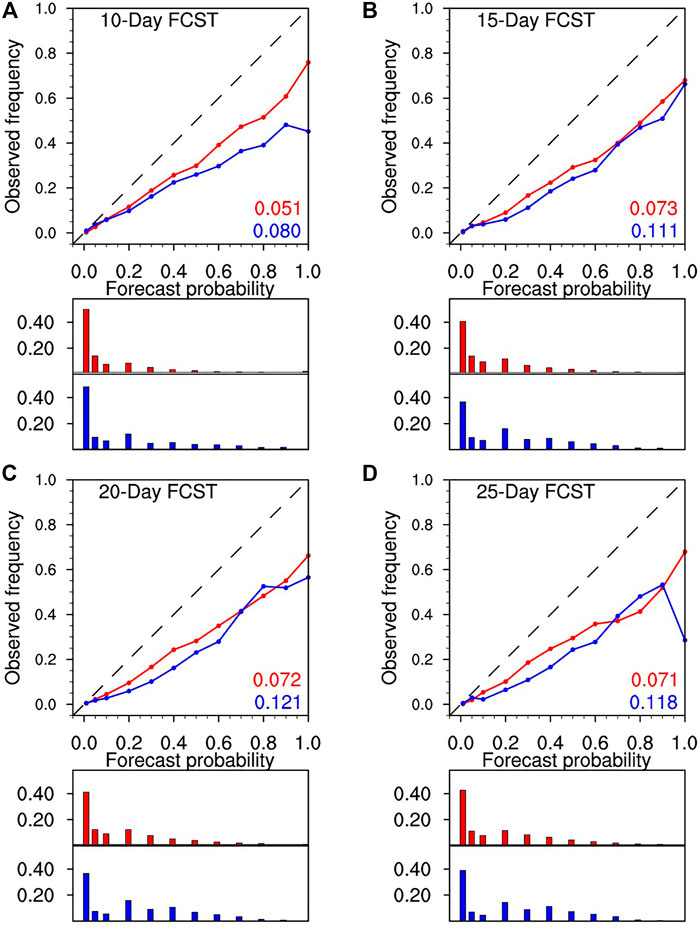
FIGURE 11. The reliability diagram for heatwave for MME (blue) and BMA (red) at lead days 10 (A), 15 (B), 20 (C), 30 (D) respectively. The forecast frequency in each probability bin is represented below on the bar plots for each forecast with the same color. The number inside each figure is the reliability which is the integral area from the diagonal line to forecast reliability line with weighting from the sample frequency.
5 Discussion and Summary
This study proposes a heatwave index (HWI) in the sub-seasonal time scale for observation and forecast. We have examined the qualification of HWI definition from available observations, which indicated that a newly defined index is able to represent heatwaves that actually occurred. On this basis, several methods are constructed for the probabilistic forecasting of HWI. We have evaluated the performance of these methods, including deterministic and probabilistic forecasts. The result shows that the probabilistic forecast performance of BMA is the best even though the deterministic performance of BMA is comparable to the MME and ECMWF. It means that the BMA model has demonstrated its value for heatwave forecast in the extended-range prediction.
The outcome of the BMA model is the daily probability of HWI in the sub-seasonal forecast. In the real-time forecast, decision-makers are more concerned about the period of a heatwave, including start date, end date, persistent days, and the probability of the whole event. This information provides decision-makers with the amount of confidence associated with heatwaves, which is valuable for deciding if, when, and how many precautionary measures should be taken. Figure 12 shows an example of transformation from the daily probability of HWI to probability of heatwave in reforecast initiated from June 19, 2010 to July 3, 2010 at grid 24°N, 113°E. In this region, there existed a significant heatwave from July 1, 2010 to July 19, 2010 shown in the below part of Figure 12. The forecasting period of a heatwave should be the days with a probability greater than 50 percent. The forecasting probability of the whole heatwave should be the average probability during this period. Taking the forecast initiated from June 19, 2010 as an example, the forecast heatwave occurs during July 3, 2010 to July 8, 2010 with the probability of heatwave equal to 82. The BMA model has successfully predicted this heatwave 12 days in advance with much higher confidence, which is confirmed by the observations. Two important points should be taken when using the HWI to predict a heatwave. First, the actual start date and end date of the heatwave may deviate by one or 2 days whatever for forecast or observation since the 5-days running average is used in the definition of HWI. Second, the heatwave defined on each point is not restrained to this point. It represents a region centered on this point with
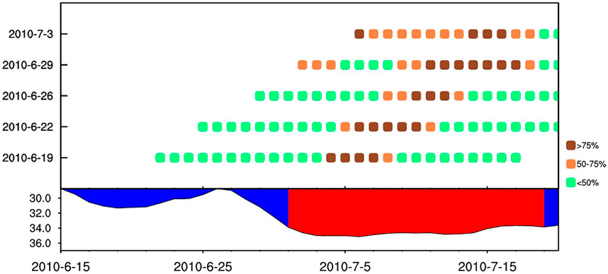
FIGURE 12. Observed HWI (lower part) and probabilistic forecasting HWI (upper part) by BMA initiated from 2010.6.19 to 2010.7.3 at grid 24°N, 113°E. Red filled area in the lower part is the observed heatwave from 2010.7.1 to 2010.7.19. The probabilistic levels are represented by different colors in the small square.
The conclusions from this study could be summarized as follows: 1). The HWI could be modified to simulate reality through observations and raw (re)forecast from the worldwide forecast system; 2). A multi-model ensemble (equal weight or poor man ensemble) could improve the forecast skills partially from comparing individual model forecasts; 3) The BMA process has demonstrated the best forecast skills around all forecasts in terms of deterministic (ensemble mean) and probabilistic forecasts (forecast reliability); 4) The implementation of HWI could present the spatial details and day-to-day hot extreme for an extended range to help to give earlier warning and/or make decisions further in advance.
Data Availability Statement
The raw data supporting the conclusion of this article will be made available by the authors, without undue reservation.
Author Contributions
JG and TS guide the ideas and techniques of the whole article, while YC and QL help deal with data.
Funding
This work is jointly supported by the National Key Program for Developing Basic Science (Grants No 2018YFC1505805 and 2018YFC1505906), the Science Foundations of China (41975102), the Open Project of the State Key Laboratory of Severe Weather, Chinese Academy of Meteorological Sciences (No. 2020LASW-B10).
Conflict of Interest
The authors declare that the research was conducted in the absence of any commercial or financial relationships that could be construed as a potential conflict of interest.
The reviewer HR declared a past co-authorship with one of the authors JG to the handling Editor.
Publisher’s Note
All claims expressed in this article are solely those of the authors and do not necessarily represent those of their affiliated organizations, or those of the publisher, the editors and the reviewers. Any product that may be evaluated in this article, or claim that may be made by its manufacturer, is not guaranteed or endorsed by the publisher.
References
Barriopedro, D., Fischer, E. M., Luterbacher, J., Trigo, R. M., and García-Herrera, R. (2011). The Hot Summer of 2010: Redrawing the Temperature Record Map of Europe. Science 332 (80), 220–224. doi:10.1080/10255842.2015.106956610.1126/science.1201224
Buizza, R., and Leutbecher, M. (2015). The Forecast Skill Horizon. Q.J.R. Meteorol. Soc. 141 (693), 3366–3382. doi:10.1002/qj.2619
Carrol, K. L., and Maloney, J. C. (2004). “Improvements in Extendedrange Temperature and Probability of Precipitation Guidance,” in Symp. 50th Anniversary of Operational Numerical Weather Prediction (College Park, MD: NWS/Amer. Meteor. Soc.).
Casanova, S., and Ahrens, B. (2009). On the Weighting of Multimodel Ensembles in Seasonal and Short-Range Weather Forecasting. Mon.Wea. Rev. 137, 3811–3822. doi:10.1175/2009MWR2893.1
Dole, R., Hoerling, M., Perlwitz, J., Eischeid, J., Pegion, P., Zhang, T., et al. (2011). Was There a Basis for Anticipating the 2010 Russian Heat Wave? Geophys. Res. Lett. 38, a–n. doi:10.1029/2010GL046582
Duncan Thompson, P. (1957). Uncertainty of Initial State as a Factor in the Predictability of Large Scale Atmospheric Flow Patterns. Tellus 9, 275–295. doi:10.3402/tellusa.v9i3.9111
Erickson, M. J., Colle, B. A., and Charney, J. J. (2012). Impact of Bias-Correction Type and Conditional Training on Bayesian Model Averaging over the Northeast United States. Wea. Forecast. 27, 1449–1469. doi:10.1175/WAF-D-11-00149.1
Fink, A. H., Brücher, T., Krüger, A., Leckebusch, G. C., Pinto, J. G., and Ulbrich, U. (2004). The 2003 European Summer Heatwaves and Drought -synoptic Diagnosis and Impacts. Weather 59 (8), 209–216. doi:10.1256/wea.73.04
Fischer, E. M., and Schär, C. (2010). Consistent Geographical Patterns of Changes in High-Impact European Heatwaves. Nat. Geosci 3, 398–403. doi:10.1038/ngeo866
Fouillet, A., Rey, G., Laurent, F., Pavillon, G., Bellec, S., Guihenneuc-Jouyaux, C., et al. (2006). Excess Mortality Related to the August 2003 Heat Wave in France. Int. Arch. Occup. Environ. Health 80, 16–24. doi:10.1007/s00420-006-0089-4
Fraley, C., Raftery, A. E., and Gneiting, T. (2010). Calibrating Multimodel Forecast Ensembles with Exchangeable and Missing Members Using Bayesian Model Averaging. Mon. Wea. Rev. 138, 190–202. doi:10.1175/2009MWR3046.1
Gneiting, T., and Katzfuss, M. (2014). Probabilistic Forecasting. Annu. Rev. Stat. Appl. 1, 125–151. doi:10.1146/annurevstatistics-062713-08583110.1146/annurev-statistics-062713-085831
Hamill, T. M., and Colucci, S. J. (1997). Verification of Eta-RSM Short-Range Ensemble Forecasts. Mon. Wea. Rev. 125 (6), 1312–1327. doi:10.1175/1520-0493(1997)125<1312:voersr>2.0.co;2
Hoag, H. (2014). Russian Summer Tops 'universal' Heatwave index. Nature. doi:10.1038/nature.2014.16250
Krishnamurti, T. N., Kishtawal, C. M., LaRow, T. E., Bachiochi, D. R., Zhang, Z., Williford, C. E., et al. (1999). Improved Weather and Seasonal Climate Forecasts from Multimodel Superensemble. Science 285, 1548–1550. doi:10.1126/science.285.5433.1548
Krzysztofowicz, R. (2001). The Case for Probabilistic Forecasting in Hydrology. J. Hydrol. 249, 2–9. doi:10.1016/S0022-1694(01)00420-6
Lin, A. L., Gu, D. J., Peng, D. D., Zheng, B., and Li, C. H. (2021). Climatic Characteristics of Regional Persistent Heat Event in the Eastern China during Recent 60 Years. J. Appl. Meteorol. Sci. 32 (3), 302–314. doi:10.11898/1001-7313.20210304
Liu, J., and Xie, Z. (2014). BMA Probabilistic Quantitative Precipitation Forecasting over the Huaihe Basin Using TIGGE Multimodel Ensemble Forecasts. Monthly Weather Rev. 142, 1520–2049. doi:10.1175/mwr-d-13-00031.1
Lorenz, E. N. (1969). Atmospheric Predictability as Revealed by Naturally Occurring Analogues. J. Atmos. Sci. 26, 636–646. doi:10.1175/1520-0469(1969)26<636:aparbn>2.0.co;2
Lorenz, E. N. (1963). Deterministic Nonperiodic Flow. J. Atmos. Sci. 20, 130–141. doi:10.1175/1520-0469(1963)020<0130:dnf>2.0.co;2
Nairn, J., Fawcett, R., and Ray, D. (2009). Defining and Predicting Excessive Heat Events, a National System. Cawcr Modelling Workshor, November 30–December 2, 2009.
Perkins, S. E., Alexander, L. V., and Nairn, J. R. (2012). Increasing Frequency, Intensity, and Duration of Observed Global Heatwaves and Warm Spells. Geophys. Res. Lett. 39, L20714. doi:10.1029/2012gl053361
Raftery, A. E., Gneiting, T., Balabdaoui, F., and Polakowski, M. (2005). Using Bayesian Model Averaging to Calibrate Forecast Ensembles. Mon. Wea. Rev. 133, 1155–1174. doi:10.1175/MWR2906.1
Richardson, D. S. (2000). Skill and Relative Economic Value of the ECMWF Ensemble Prediction System. Q.J.R. Meteorol. Soc. 126, 649–667. doi:10.1002/qj.49712656313
Schär, C., Vidale, P. L., Lüthi, D., Frei, C., Häberli, C., Liniger, M. A., et al. (2004). The Role of Increasing Temperature Variability in European Summer Heatwaves. Nature 427, 332–336. doi:10.1038/nature02300
Schiermeier, Q. (2018). Droughts, Heatwaves and Floods: How to Tell when Climate Change Is to Blame. Nature 560, 20–22. doi:10.1038/d41586-018-05849-9
Schmeits, M. J., and Kok, K. J. (2010). A Comparison between Raw Ensemble Output, (Modified) Bayesian Model Averaging, and Extended Logistic Regression Using ECMWF Ensemble Precipitation Reforecasts. Mon. Wea. Rev. 138, 4199–4211. doi:10.1175/2010MWR3285.1
Shi, J., Ding, Y. H., and Cui, L. L. (2008). The Climatic Characteristics and Their Changing Law during Summer High-Temperature Times in East China. ACTA Geographica Sinica 63 (3), 237–246. (in Chinese). doi:10.3321/j.issn:0375-5444.2008.03.002
Sloughter, J. M., Gneiting, T., and Raftery, A. E. (2010). Probabilistic Wind Speed Forecasting Using Ensembles and Bayesian Model Averaging. J. Am. Stat. Assoc. 105 (489), 25–35. doi:10.1198/jasa.2009.ap08615
Sloughter, J. M. L., Raftery, A. E., Gneiting, T., and Fraley, C. (2007). Probabilistic Quantitative Precipitation Forecasting Using Bayesian Model Averaging. Mon. Wea. Rev. 135 (9), 3209–3220. doi:10.1175/mwr3441.1
Smagorinsky, J. (1969). Problems and Promises of Deterministic Extended Range Forecasting1. Bull. Amer. Meteorol. Soc. 50, 286–312. doi:10.1175/1520-0477-50.5.286
Stauffer, R., Umlauf, N., Messner, J. W., Mayr, G. J., and Zeileis, A. (2017). Ensemble Postprocessing of Daily Precipitation Sums over Complex Terrain Using Censored High-Resolution Standardized Anomalies. Mon. Wea. Rev. 145, 955–969. doi:10.1175/MWR-D-16-0260.1
Trigo, R. M., García-Herrera, R., Díaz, J., Trigo, I. F., and Valente, M. A. (2005). How Exceptional Was the Early August 2003 Heatwave in France. Geophys. Res. Lett. 32, L10701. doi:10.1029/2005GL022410
Vitart, F., Ardilouze, C., Bonet, A., Brookshaw, A., Chen, M., Codorean, C., et al. (2017). The Subseasonal to Seasonal (S2S) Prediction Project Database. Bull. Am. Meteorol. Soc. 98, 163–173. doi:10.1175/BAMS-D-16-0017.1
Vitart, F., and Robertson, A. W. (2018). The Sub-seasonal to Seasonal Prediction Project (S2S) and the Prediction of Extreme Events. Npj Clim. Atmos. Sci. 1, 3. doi:10.1038/s41612-018-0013-0
Weisheimer, A., and Palmer, T. N. (2014). On the Reliability of Seasonal Climate Forecasts. J. R. Soc. Interf. 11 (96), 20131162–20131210. doi:10.1098/rsif.2013.1162
White, C. J., Carlsen, H., Robertson, A. W., Klein, R. J. T., Lazo, J. K., Kumar, A., et al. (2017). Potential Applications of Subseasonal-To-Seasonal (S2S) Predictions. Met. Apps 24, 315–325. doi:10.1002/met.1654
Xia, J., Tu, K., Yan, Z., and Qi, Y. (2016). The Super-heat Wave in Eastern China during July-August 2013: a Perspective of Climate Change. Int. J. Climatol. 36, 1291–1298. doi:10.1002/joc.4424
Zhu, Y., Toth, Z., Wobus, R., Richardson, D., and Mylne, K. (2002). The Economic Value of Ensemble-Based Weather Forecasts. Bull. Amer. Meteorol. Soc. 83 (1), 73–83. doi:10.1175/1520-0477(2002)083<0073:tevoeb>2.3.co;2
Keywords: extended-range forecast, probabilistic forecast, S2S, BMA, Heat Wave
Citation: Zhang W, Gao J, Lai Q, Chi Y and Su T (2022) Probabilistic Forecast of the Extended Range Heatwave Over Eastern China. Front. Earth Sci. 9:810579. doi: 10.3389/feart.2021.810579
Received: 07 November 2021; Accepted: 06 December 2021;
Published: 05 January 2022.
Edited by:
Guihua Wang, Fudan University, ChinaReviewed by:
Yuejian Zhu, NCEP Environmental Modeling Center (EMC), United StatesJiacan Yuan, Fudan University, China
Hong-Li Ren, Chinese Academy of Meteorological Sciences, China
Copyright © 2022 Zhang, Gao, Lai, Chi and Su. This is an open-access article distributed under the terms of the Creative Commons Attribution License (CC BY). The use, distribution or reproduction in other forums is permitted, provided the original author(s) and the copyright owner(s) are credited and that the original publication in this journal is cited, in accordance with accepted academic practice. No use, distribution or reproduction is permitted which does not comply with these terms.
*Correspondence: Jianyun Gao, ZnpnYW9qeXVuQDE2My5jb20=