Multi-Scale X-Ray Computed Tomography Analysis to Aid Automated Mineralogy in Ore Geology Research

Ore characterization is crucial for efficient and profitable production of mineral products from an ore deposit. Analysis is typically performed at various scales (meter to microns) in a sequential fashion, where sample volume is reduced with increasing spatial resolution due to the increasing costs and run times of analysis. Thus, at higher resolution, sampling and data quality become increasingly important to represent the entire ore deposit. In particular, trace metal mineral characterization requires high-resolution analysis, due to the typical very fine grain sizes (sub-millimeter) of trace metal minerals. Automated Mineralogy (AM) is a key technique in the mining industry to quantify process-relevant mineral parameters in ore samples. Yet the limitation to two-dimensional analysis of flat sample surfaces constrains the sampling volume, introduces an undesired stereological error, and makes spatial interpretation of textures and structures difficult. X-ray computed tomography (XCT) allows three-dimensional imaging of rock samples based on the x-ray linear attenuation of the constituting minerals. Minerals are visually differentiated though not chemically classified. In this study, decimeter to millimeter large ore samples were analyzed at resolutions from 45 to 1 μm by AM and XCT to investigate the potential of multi-scale correlative analysis between the two techniques. Mineralization styles of Au, Bi-minerals, scheelite, and molybdenite were studied. Results show that AM can aid segmentation (mineralogical classification) of the XCT data, and vice versa, that XCT can guide (sub-)sampling (e.g., for heavy trace minerals) for AM analysis and provide three-dimensional context to the two-dimensional quantitative AM data. XCT is particularly strong for multi-scale analysis, increasingly higher resolution scans of progressively smaller volumes (e.g., by mini-coring), while preserving spatial reference between (sub-)samples. However, results also reveal challenges and limitations with the segmentation of the XCT data and the data integration of AM and XCT, particularly for quantitative analysis, due to their different functionalities. In this study, no stereological error could be quantified as no proper grain separation of the segmented XCT data was performed. Yet, some well-separated grains exhibit a potential stereological effect. Overall, the integration of AM with XCT improves the output of both techniques and thereby ore characterization in general.

Introduction

Mineralogical investigations are crucial in both the mining industry and ore geology research to understand the fundamental processes behind the formation of ore deposits. This type of investigation is necessary to optimize exploration for new deposits and production efficiency of existing mines. As knowledge of ore deposits increases, details become increasingly relevant. Over the last few decades, analytical techniques (including automated ones) have been continuously developed and improved such that they now enable study of ore deposits down to the nanoscale (Reich et al., 2017). Several automated scanning electron microscopy systems have been developed (QEMSCAN, MLA, Mineralogic, TIMA, AMICS, INCA Mineral), collectively referred to as Automated Mineralogy (AM), to rapidly scan and classify samples (e.g., polished thin sections, epoxy mounts) concerning their mineralogy based on backscattered electron (BSE) imaging and energy dispersive x-ray spectroscopy (EDS; Schulz et al., 2020). This allows quantification of geological and geometallurgical parameters such as mineral composition, mineral association, grain size distribution, degree of liberation, etc. Yet, AM has several drawbacks. 1) Cost and time of analysis increase with spatial resolution, thus generally only small sample areas (mm²-cm²) and a limited number of samples are analyzed. A sample selection suitable for its purpose is therefore critical. 2) Sample preparation is destructive and requires cutting and grinding of a larger sample (e.g., drill core). This causes loss of material and hence loss of potentially important information. 3) AM is limited to two-dimensional analysis, and thus requires that the geologist translates the two-dimensional observations into the third dimension (Baker et al., 2012). For rocks of complex mineralogy, textures, and structures, this can be challenging. In addition, quantitative data is subject to stereological error (Lätti & Adair 2001; Sutherland 2007), which is especially pronounced for preferably oriented mineral grains (low variability in the cutting plane relative to the crystal lattice) and trace minerals (nugget effect). Despite their low abundance, trace minerals can be significant to a mining venture if they contain metals of high economic value, either as main commodity or as by-products (e.g., Au, Ag), critical metals (e.g., Critical Raw Material; European Commission 2020), or penalty elements (e.g., As, Hg, U, Sb). In addition, detailed mineralogical knowledge of an ore deposit supports its ore genetic classification, which is an important input into any mineral exploration campaign. Hence, good control on trace metal mineral occurrence and distribution in an ore deposit is crucial.

An excellent tool to address the mentioned drawbacks is X-ray Computed Tomography (XCT), which allows the visualization of samples in 3D. A sample is placed between an x-ray source and a detector and rotated 360° around a vertical axis. A cone-shaped x-ray beam penetrates and is attenuated by the sample. The detector collects the transmitted x-rays, which provide information on the x-ray linear attenuation. Based on the variation of the x-ray attenuation as the sample rotates an x-ray linear attenuation coefficient is calculated for each voxel (3D pixel) in the sample. This coefficient is displayed as a distinct grey scale value in the XCT dataset, which is a cubical matrix of grey scale values. The x-ray linear attenuation coefficient depends on the density and element composition of the material analyzed and thus allows differentiation between minerals if their attenuation coefficients are sufficiently different. A detailed description of the XCT technique and its application in geoscience is provided in several reviews (e.g., Baker et al., 2012; Cnudde and Boone 2013; Godel 2013; Kyle and Ketcham 2015; Hanna and Ketcham 2017; Guntoro et al., 2019a; Wang and Miller 2020; Withers et al., 2021). XCT is non-destructive and applicable over a wide range of scales (meter to nanometer; Wang and Miller 2020), enabling scanning of entire drill core sections and to preserve their mineralogical, textural, and structural information prior to subsample production (thin section, rock chip, etc.) for 2D micro-analysis. The XCT data can aid in selecting regions of interest for micro-analysis and in correlating surface features of subsamples with their original position in the drill core. Drill cores are ideally suited for XCT analysis, due to their cylindrical shape. This allows consistent sample thickness between x-ray source and detector as the sample rotates 360° during analysis. Further, the cut-off-material of subsamples, the subsamples themselves, and smaller regions of interest therein can subsequently be re-scanned with higher resolution XCT for more detailed analysis, e.g., the study of individual mineral grains (Godel 2013). In the oil industry, XCT analysis of drill cores is performed routinely (Butcher 2020), e.g., to quantify the pore volume and its interconnectivity. Further, mini-cores are subsequently drilled from the larger cores for higher-resolution analysis (Butcher 2020). However, XCT analysis and mini-coring are yet uncommon in the mining industry. This may partly be due to the typically more complex mineralogy and texture of ore-forming rocks compared to oil-bearing sandstones and shales.

A major challenge with XCT is quantitative mineral analysis. This requires segmentation of the various minerals from the grey scale images. Difficulties arise since the grey scale value of a voxel, which represents an x-ray linear attenuation coefficient, is not only dependent on the x-ray attenuation of a mineral. Various artefacts influence x-ray attenuation across a sample, including but not limited to: 1) beam hardening, an increase in average beam energy along a ray path caused by the higher absorption of low-energetic (soft) x-rays compared to high-energetic (hard) x-rays within a sample. Beam hardening results in a gradient of the reconstructed x-ray linear attenuation coefficient towards the center of the sample (cupping effect, Cnudde and Boone 2013). 2) Streak artefacts, bright and dark streaks emanating from a highly attenuating phase into the surrounding material due to beam hardening (De Man et al., 1998; Kyle and Ketcham 2015). 3) X-ray attenuation reconstruction errors vertically away from the centre of a sample due to the conical shape of the x-ray beam (cone-beam effect; Cnudde and Boone 2013). 4) Ring artefacts caused by differences in sensitivity of the detector elements (Cnudde and Boone 2013; Kyle and Ketcham 2015). In addition, voxels may intersect multiple phases and represent mixed attenuation coefficients (Partial Volume Effect; Ketcham and Carlson 2001; Hanna and Ketcham 2017). A voxel may contain contributions from surrounding voxels due to machine- and acquisition-dependent factors, an effect known as blurring (Hanna and Ketcham 2017). Moreover, minerals of solid solution series and chemically zoned mineral grains may exhibit a range of x-ray linear attenuation coefficients, dependent on the exact chemical composition (Kyle and Ketcham 2015). All this causes the voxels of a mineral grain to range in grey scale values and to overlap with the grey scale values of other mineral grains, particularly if their theoretic x-ray linear attenuation coefficients are similar. Visual inseparability in the XCT dataset may be a result. The x-ray linear attenuation coefficient of a mineral varies with x-ray energy (Berger et al., 2010; Godel 2013; Reyes et al., 2017). The variation is not the same for all minerals, thus visual separability of some minerals may be increased by altering the x-ray energy used for analysis. One solution to improve separability of all minerals is to combine multiple scans at different energies. Nevertheless, segmentation of XCT data in general is much more limited compared with e.g. AM.

For segmentation of XCT data several methods exist, varying in complexity and computational intensity (Godel 2013; Wang and Miller 2020). The simplest is grey scale thresholding based on peaks in the histogram. This method is fast but due to the above-mentioned overlap between minerals prone to errors (Godel 2013; Wang and Miller 2020). It can be improved through combination with an edge intensity filter (e.g., Sobel) and the watershed algorithm (Godel 2013; Guntoro et al., 2019a; Wang and Miller 2020). This ‘histographic segmentation’ is also rapid and works well for samples with distinct grain boundaries but struggles with fine-grained and complex textures. Superior results are achieved by use of machine learning, yet these require sufficient training data, heavy computation power, and dedicated time spent on optimization (Godel 2013; Reyes et al., 2017; Guntoro et al., 2019b). In the end, the limitations of too similar x-ray linear attenuation coefficients apply to all segmentation methods. Nevertheless, some quantification of mineral volumes, association, grain sizes, orientation, etc. is possible and may supplement 2D quantitative data.

In this study, multi-scale (45, 30, 4, and 1 μm) XCT and AM analyses were performed on polished and epoxy mounted drill core rock chips of ore from the Liikavaara Östra Cu-(W-Au) deposit, northern Sweden. Correlation and integration of both techniques across the various scales were investigated. Focus was on the modal mineralogy, detection of heavy trace minerals, and textures. The benefits and challenges of multi-modal and multi-scale analysis for ore characterization are discussed.

Geological Background

The samples investigated in this study are from the Liikavaara Östra Cu-(W-Au) deposit in northern Sweden. It is an intrusion-related vein-style deposit hosted by Paleoproterozoic meta-volcanoclastic rocks (Warlo et al., 2020). Boliden AB has scheduled the deposit for production in the coming years. Copper, hosted in chalcopyrite, will be the main commodity, and Au and Ag will be by-products. Molybdenum and the critical metals W and Bi are also enriched, though only Mo is currently considered a potential future by-product. The ore minerals are mainly hosted by quartz-(tourmaline-calcite) veins often within or in proximity to aplite dykes (Warlo et al., 2020). The precious metals are of diverse mineralogy. Gold occurs natively and as a Au-Ag-alloy; Ag also occurs as tellurides and sulfides (Warlo et al., 2020). The Au and Ag minerals are fine-grained (mainly <10 μm for Au, and <50 μm for Ag). They are found as inclusions within, and in contact with, chalcopyrite and gangue (mainly quartz and other sulfides). Gold is also associated with micron-sized grains of native Bi (Warlo et al., 2020). The only Mo-bearing mineral is molybdenite, grains of which are typically tens of microns to a few millimeter in size and associated with quartz, sulfides, scheelite, and calcite (Warlo et al., 2020). Previous analysis by scanning electron microscopy with energy dispersive spectrometry (SEM-EDS) and synchrotron radiation x-ray fluorescence mapping (SR-XFM), showed molybdenite to be rich in micron-to nano-inclusions (Warlo et al. submitted). The inclusions are trapped in cavities between striations in the molybdenite grains and are chemically diverse but mainly composed of Fe-oxides, Fe-silicates, and Bi-(Pb-Se), but also Au-Ag, and Ag-Te. In addition, SR-XFM revealed the existence of lattice-bound impurities of Re, Se, and W in molybdenite (Warlo et al. submitted). Scheelite is the only major W-bearing mineral and commonly confined to the quartz-dominated part of quartz-(tourmaline-calcite) veins. Scheelite grains are mostly larger (several millimeters in width) than associated mineral grains and typically fractured (Warlo et al., 2020).

Samples and Methods

The samples were a ∼20 cm long half drill core piece, four polished and epoxy-mounted cylindrical rock chips of ∼30 mm diameter and 12 mm in height, and two mini cores of 4 mm diameter and 10 mm in height (Figure 1). The samples were cut from three drill cores that intersect the ore zone of the Liikavaara Östra Cu-(W-Au) deposit. Drill core logging and routine chemical assays from Boliden AB on metals of economic, environmental, and metallurgical interest, guided the sampling. The focus was on representative samples for the mineralization of Au, Mo, and W. Four styles of mineralization were sampled:

1) Scheelite-bearing aplite dyke.

2) Sulfide-rich quartz-(calcite-tourmaline) vein. The chemical assays for this structure were 6 ppm Au and 10.4 ppm Ag content, over a 1.3 m section.

3) A second aplite dyke that contains thin quartz veins rich in molybdenite and scheelite.

4) Contact between a quartz vein and host biotite schist. Molybdenite mineralization occurs along the contact within the quartz vein.

FIGURE 1

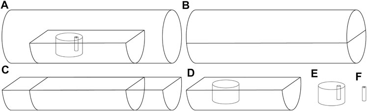
FIGURE 1. Schematic drawings of the sampling and analysis methodology of this study. (A) Overview of all a sample types in their relation to the original drill core. (B) A drill core is cut in half. One half core is analyzed by whole rock XRF and the other half is logged. (C) The logged half core is subsampled. In this study, an XCT scan at 45 μm voxel size was performed on one subsampled half core (2). (D) A rock chip is cut from the half core sample, polished, and epoxy-mounted. In this study, XCT scans at 30 μm voxel size were performed on four rock chips and 30 μm pixel size AM scans on their polished surface (1–4). (E) A mini core is drilled from the rock chip sample. In this study, XCT scans at 4 μm voxel size were performed on two mini cores and 1 μm pixel size AM scans on their polished surface prior to drilling (2, 3). (F) A cylindrical volume of interest within the mini core is selected for XCT analysis. In this study, XCT scans at 1 μm voxel size were performed in volumes of interest in two mini cores (2, 3).

For each mineralization style, one epoxy-mounted rock chip was prepared. For sample 2, the rock chip was cut from the half drill core piece also analyzed in this study. The two mini cores were drilled from the rock chips of samples 2 and 3, respectively (Figure 1E). The creation of mini cores was necessary to achieve a short distance between the x-ray source and the samples, and thereby allow high-resolution XCT analysis.

Automated Mineralogy

The polished surface of each of the four epoxy-mounted rock chips was scanned by AM using a Zeiss Sigma 300 VP with two EDS detectors and the Mineralogic software at Luleå University of Technology (Table 1). A pixel size (beam sampling distance) of 30 μm was chosen; a trade-off between resolution and time spent on analysis. Two regions of interest (4 mm diameter) in the rock chips of samples 2 and 3, subsequently drilled for extraction of the mini cores, were additionally scanned at 1 μm pixel size (Table 1). The same custom-made mineral library in the Mineralogic software was used for initial mineral classification in all scans. Element filters for Au, Ag, and Bi were placed at the top of the mineral library to identify sub-pixel sized grains of trace metal minerals recorded as mixed phase spectra (Warlo et al., 2019). Results were processed in the Mineralogic Explorer software. Here, mineral maps were stitched and montaged and quantitative data on bulk mineralogy, mineral association, metal deportment, were extracted. The accuracy and precision of the mineral library was assessed by manual spot-checking the BSE image and respective EDS spectra of the identified minerals. For Au and Ag minerals, every pixel found was reviewed. Based on this assessment, the mineral library was then fine-tuned for each scan and data reclassified.

TABLE 1

TABLE 1. Experimental conditions of AM and XCT. For XCT analysis, the half drill core piece was analyzed on a GE phoenix v|tome|x s at GTK, Espoo, Finland. All other samples were analyzed on a Zeiss Xradia 510 Versa at LTU, Luleå, Sweden.

For comparison with XCT, the detailed mineral maps were subsequently simplified based on the limiting number of segmented classes in the XCT scans. The Mineral X-Ray Linear Attenuation Coefficient Tool (MXLAC) by Bam et al. (2020) was used to calculate the mineral x-ray linear attenuation coefficient of each mineral for the respective beam energy used in the XCT analysis. All minerals identified by AM where ranked accordingly. For certain mineral groups (e.g., amphibole, epidote), the attenuation coefficient of only one mineral from the group was calculated to represent the whole group. For broader-defined groups (e.g., silicates, Fe-oxides/carbonates), no values were calculated but the approximate position in the ranking estimated. The coefficients were then used in conjunction with visual comparisons of AM and XCT images to assign the minerals to the classes segmented in the XCT scans (Table 2).

TABLE 2

TABLE 2. List of calculated x-ray linear attenuation coefficients of all minerals identified by AM in this study. The colors in the left column (Mineral) refer to the respective colors of the minerals in the AM mineral maps. The numbers in the columns are the x-ray linear attenuation coefficients of the minerals for the respective beam energy of each scan (175, 160, 140 and 80 kV). The coefficients were calculated using the MXLAC tool (Bam et al., 2020). For mineral groups (e.g., amphiboles, epidote) one mineral was picked to represent the whole group. For broad groups (e.g., silicates, Fe-oxides/carbonates) no values were calculated. The XCT data were segmented into classes (mineral groups) based on a combination of grey-scale thresholding and an edge intensity filter. To determine the minerals comprising each segmented class, the data were visually compared with the AM mineral maps. Each mineral from the original AM maps was then appointed to its corresponding class (mineral group) in the segmented XCT data and simplified AM mineral maps created. For minerals where visual comparison of the AM and XCT data was inconclusive to appoint it to a class, the calculated x-ray linear attenuation coefficient relative to that of the other minerals was used as reference. Color coding of the cells with numbers represents the simplification of the AM quantitative maps for correlation with the segmented XCT data. Uncolored cells indicate that the minerals were not present in the respective AM maps. Variable contrast between minerals in the XCT data due to variable beam energies, tomographic reconstruction, and beam hardening correction between XCT scans is the reason for the differences in mineralogy of the segmented classes between scans.

Since Mineralogic Explorer does not offer an option for analysis of subregions within a scan, the simplified quantitative maps were converted into grey scale images, imported into ORS Dragonfly, and re-segmented based on their histograms. This allowed overlay of the AM data with the XCT data and quantitative analysis of the same region. For the epoxy-mounted rock chip scans, a circular/cylindrical (AM/XCT) region was chosen, which maximized area/volume while excluding the border between rock and epoxy. For the high-resolution scans, an area/volume that maximized the overlap between the 1 μm pixel size mineral maps and the XCT scans of the mini cores was chosen.

The AM data of the 1 μm pixel size scan of sample 2 became corrupted after reclassification with the updated mineral library. Results were still accessible but further reclassification was no longer possible. This caused issues with simplification of the mineralogy for comparison with XCT. Some minerals initially colored the same could no longer be separated. This was the case for Fe-oxides (ilmenite, magnetite, hematite, FeO, Fe-oxides/carbonates) and tin minerals (cassiterite, tin minerals). They were therefore treated together according to the mineral of highest concentration (Fe-oxides/carbonates and tin minerals, respectively). Quantitatively, the miss-classified Fe-oxides covered ∼0.2 area % and cassiterite <0.01 area % in the whole mineral map. Since no equivalent quantitative data could be inferred for the region compared with XCT, no correction was performed. Regardless, impact on the quantitative comparison was minimal.

X-Ray Computed Tomography

The half drill core piece was scanned by XCT at 45 μm voxel size using a GE phoenix v|tome|x s at the Geological Survey of Finland, Espoo, Finland (Table 1). The four epoxy-mounted rock chips were scanned at 30 μm voxel size using a Zeiss Xradia 510 Versa at Luleå University of Technology (Table 1). Two rock chips each (samples 1 and 2, and 3 and 4) were stacked with their polished surfaces face to face, fixed in place with tape, and analyzed together (see Supplementary Figure S1). This was to minimize the cone-beam effect on the polished surfaces of the samples. The two mini drill cores were also analyzed with the Zeiss Xradia 510 Versa at 4 μm voxel size. In addition, a cylindrical volume of interest of 1 mm in both diameter and height within each 4 mm drill core was scanned at 1 μm voxel size. The Zeiss Xradia system has multiple detector objectives enabling sample imaging at a number of resolution and field of view pairings. Here, the rock chip samples were scanned using a ×0.4-objective, while the mini drill core samples were scanned using a ×4-objective, specified more in detail in Table 1.

The tomographic reconstruction was carried out using filtered back projection, and beam hardening correction applied where necessary. However, due to the complex mineralogy within the samples (large range of x-ray linear attenuation coefficients) optimization for all minerals was not possible. Hence, corrections and filters commonly were applied in favor of the higher x-ray linear attenuation coefficients (denser minerals) as these were in focus in this study.

The XCT data were processed and analyzed using the software ORS Dragonfly (version 2021.1). Images of the raw XCT data are shown in Supplementary Figures S1,S2. Image processing was performed on each data set prior to mineral segmentation. The ‘Unsharp’ filter was applied to increase edge contrast of grains, followed by the ‘Mean Shift’ filter to smoothen the noise introduced by the ‘Unsharp’ filter. Segmentation was performed on a cylindrical subvolume in each data set, so that: 1) the epoxy mount was excluded 2) depth-related grey scale gradients (e.g., cone-beam effect), did not affect segmentation significantly, 3) each horizontal slice was of equal area, and 4) the top slice overlapped with the respective mineral map from AM. The only exception was the half drill core piece where segmentation was performed on a half cylinder partly including the contact with the surrounding air. The ‘Histographic Segmentation’ plug-in in the ORS Dragonfly software was used for mineral segmentation. This plug-in includes a combination of grey scale thresholding and the sobel filter to define classes (groups of minerals of similar x-ray linear attenuation coefficient) and determine markers in the sobel image for the watershed algorithm (Guntoro et al., 2019a). Individual grains were determined based on a 6-point particle connection (shared voxel faces). Heavy trace minerals in the samples of mineralization style 2 were of too low volume to be identified accurately by ‘Histographic Segmentation’. Hence, the trace minerals were segmented by manual grey scale thresholding. The ‘Histographic Segmentation’ (and grey scale thresholding) were performed six times for each sample to get an estimate of the standard deviation for the various segmented phases.

The segmented XCT data were used for quantitative analysis. The mean bulk volumes of the segmented mineral classes and their respective area percentage in each horizontal slice were calculated for the six segmentations of each scan. The mean data of the slices overlapping with the mineral maps were used for quantitative comparison between XCT and AM. In addition, the grey scale and segmented XCT images were visually inspected concerning texture and structure of the ore samples.

Results

The AM scans provide detailed mineral maps of the 2D surface of the rock chip samples, complemented with 3D-spatial data from XCT analysis. Below are the results of scans of the four samples: 1) ‘scheelite- and Bi-telluride-bearing aplite’, 2) ‘gold-bearing sulfide-rich quartz vein’, 3) ‘molybdenite- and scheelite-bearing quartz veins in aplite’, and 4) ‘molybdenite-rich contact between a quartz vein and biotite schist’, presented and illustrated in detail.

Scheelite- and Bi-Telluride-Bearing Aplite (Sample 1)

The AM scan shows the contact between biotite schist and an intruding aplite dyke (Figure 2). The aplite dyke contains several up to ∼4.5 mm sized scheelite grains together with chalcopyrite and pyrrhotite. Several sub-millimeter inclusions of Bi-tellurides occur in the pyrrhotite. Some ambiguity on pixel classification exists in very fine-grained regions, e.g., the biotite schist, due to mixed EDS spectra. Overall, mineral classification and resolution of textures agree with previous observations from reflected light microscopy and SEM-EDS. In the XCT scan only four classes (mineral groups) can be visually separated, 1) silicates and carbonates, 2) sulfides and oxides, 3) scheelite, and 4) heavy minerals (mostly Bi-tellurides; Figure 2, Table 3). Comparison of the top slice of the segmented XCT data with the same area in the AM mineral map shows considerable quantitative differences (Table 3). Although total difference in area between the techniques are largest for the silicates/carbonates (∼11%), the relative difference is much larger for the heavy minerals (∼70%) due to their overall low abundance (Table 3). The sulphides/oxides are high in both total and relative area difference. The differences can be explained mainly by the effect of streak artefacts in the XCT data, caused by the scheelite and heavy mineral grains, on the histographic segmentation. This results in spurious aureoles of sulfides/oxides around scheelite and heavy mineral grains (Figures 2, 3). Additionally, some scheelite grains have brighter rims than cores, which causes segmentation of the rims into the class of heavy minerals (Figures 2, 3). Segmentation of regions without scheelite grains appear satisfactory. Texturally, the unaided eye and AM indicate a preferred planar orientation of scheelite and sulfides within the quartz vein (Figure 2). XCT confirms this and shows continuity of the scheelite vein deep into the sample. Scheelite grains are relatively large (∼7 mm) and elongated towards depth but strongly fractured (Figure 3). Heavy minerals mainly form inclusions within the sulfides. The XCT images clearly display the dissemination of heavy mineral inclusions and the problem with grain size estimations based on 2D sections. The largest Bi-telluride grain observed on the polished surface by AM (∼0.5 mm) is intersected at an edge and grows considerably larger with depth in the sample (∼2.5 mm) (Figure 3). This also exceeds previously reported maximal grain sizes of Bi-minerals (0.5 mm) at the Liikavaara Östra Cu-(W-Au) deposit (Warlo et al., 2020).

FIGURE 2

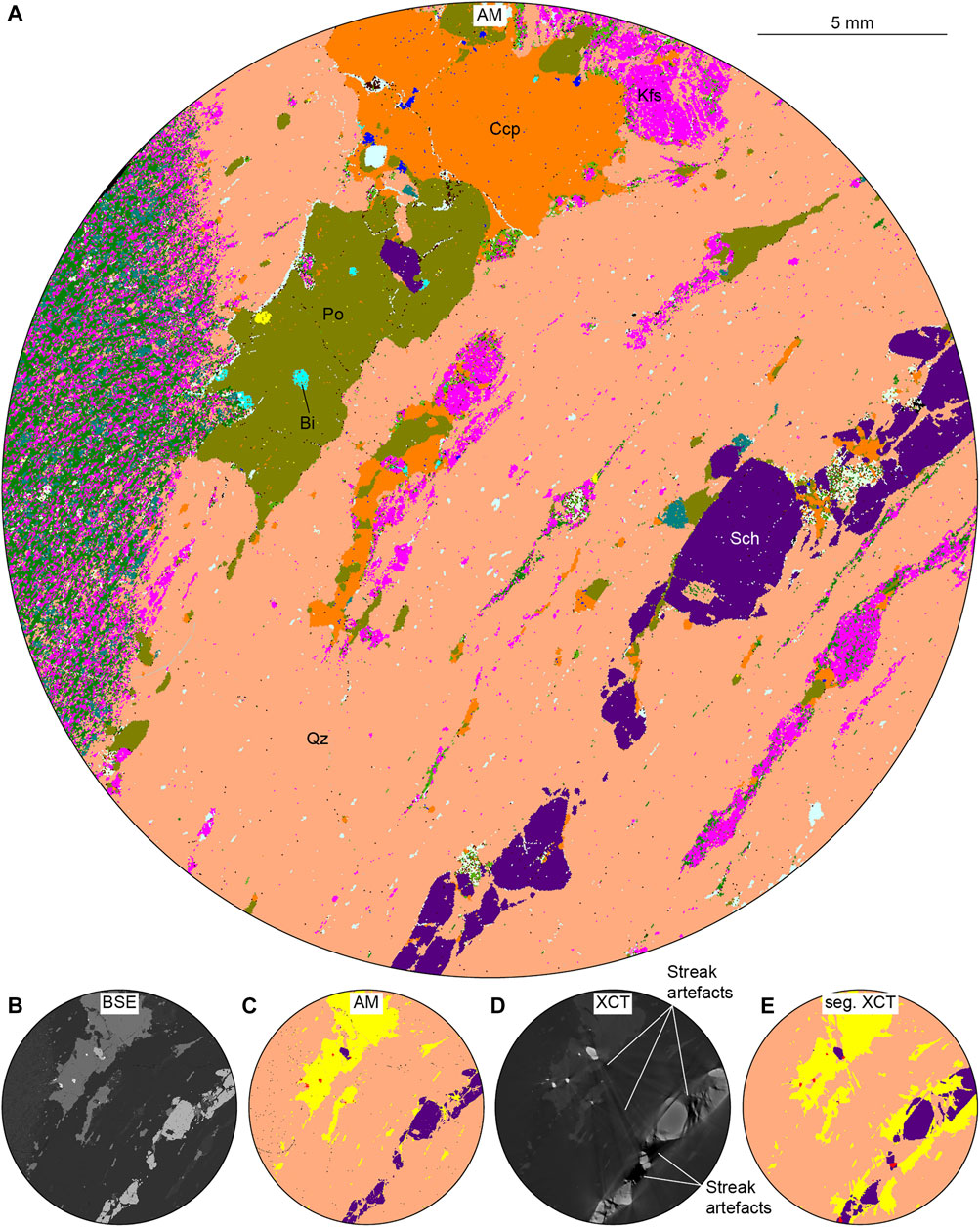
FIGURE 2. AM and XCT images of a polished rock chip of a scheelite- and Bi-telluride-bearing aplite (sample 1). For color coding of the minerals see Table 2. (A) 30 μm pixel size AM mineral map. (B) 1.87 μm pixel size AM BSE image. (C) 30 μm pixel size simplified AM mineral map. (D) 30 μm voxel size XCT scan. (E) 30 μm voxel size segmented XCT scan. Streak artefacts of scheelite and Bi-mineral grains in the XCT scan (D) cause segmentation of scheelite grain boundaries as heavy minerals, quartz as sulfides (bright streaks), and sulfides as quartz (dark streaks). Abbreviations: Ccp – chalcopyrite, Kfs – k-feldspar, Po – pyrrhotite, Sch – scheelite, Qz – quartz.

FIGURE 3

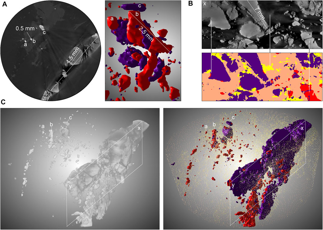
FIGURE 3. XCT images of the rock chip of sample 1. For color coding of the minerals, see Table 2. (A) Grains of Bi-telluride (a, b) and scheelite (c) within pyrrhotite in the top slice of the sample (left). 3D segmented volumes of the same grains in 3D viewed at a close to 90° pitch (right). Especially grain ‘b’ has a much larger size than may be presumed from the 2D slice. (B) Profile along the scheelite vein. Scheelite grains are partly elongated towards depth and fractured. Variation in the grey scale due to streak artefacts (top) results in the margins or entire grains of scheelite to be segmented as heavy minerals and parts of quartz as sulfides (bottom). (C) 3D-rendered volumes of scheelite and heavy minerals (Bi-tellurides) based on the x-ray attenuation data (left) and segmentation (right). The yellow and pink dots in the segmented image (right) show the rough outline of the sulfides and quartz, respectively. The large heavy minerals in the scheelite vein are likely wrongly segmented scheelite grains (see (B)).

TABLE 3

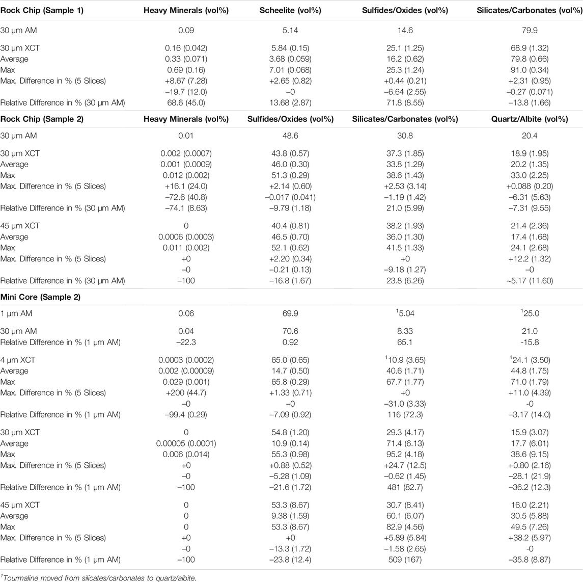
TABLE 3. Comparison of the area fraction of the classes segmented in the rock chip of samples 1 and 2 between the AM mineral map and the corresponding XCT slice. Additionally, the maximal difference in percent between the XCT slice used for comparison with AM and the following four slices is shown. Average and Max values refer to all slices within a specific segmented volume (rock chip, mini core) of an XCT data set. The XCT values are the mean values of six segmentations (n = 6) of the same volume, with the standard deviation in brackets. A minimal error (<0.2 area %) may occur for the 1 μm AM data of sample 2 due to file corruption (see section Automated Mineralogy).

Gold-Bearing Sulfide-Rich Quartz Vein (Sample 2)

The XCT scan of the half drill core shows a complex intergrowth of sulfide and gangue minerals (Figure 4). The undifferentiated sulfides mainly occur to one side of the core. The gangue can be differentiated into a dark grey fine-grained matrix replacing larger fractured grains of even darker grey. Very bright heavy mineral grains occur scattered within the gangue. These bright phases are likely galena and/or scheelite, based on the relatively large grain sizes compared with other heavy minerals in the Liikavaara Östra Cu-(W-Au) deposit (Warlo et al., 2020). To target the Au mineralization, the rock chip was taken from the sulfide-dominated part of the drill core. Although the XCT scan of the half core shows only few bright phases in this region (Figure 4), this is to be expected considering the generally small grain size of Au minerals (Warlo et al., 2020).

FIGURE 4

FIGURE 4. XCT images of the drill core piece, rock chip, and mini core of sample 2. For color coding of the minerals, see Table 2. (A) Segmented XCT images of the various scans (45, 30, 4, and 1 μm voxel size) along the three spatial axes. (B) Opaque (top) and transparent (bottom) 3D-rendered XCT images of the drill core piece, rock chip, and mini core. The black and dark grey phases correspond mainly to silicates and carbonates, the medium grey phases to sulfides, and the bright phases to heavy minerals (e.g., scheelite, galena, Au- and Bi-minerals). (C) 3D-rendered XCT image of the rock chip (30 μm voxel size). The sulfides are rendered transparent to better reveal the heavy mineral inclusions (bright grains). (D) 3D-rendered XCT image of the mini core (4 μm voxel size). The sulfides are rendered transparent to better reveal the heavy mineral inclusions (bright grains). (E) 3D-rendered XCT image of the volume of interest within the mini core (1 μm voxel size). The sulfides are rendered transparent to better reveal the heavy mineral inclusions (bright grains).

AM of the surface of the rock chip resolves the mineralogy in better detail compared with XCT (Figure 5). A fine-grained matrix of mainly biotite, chlorite, ankerite, quartz, and Fe-oxides/carbonates, with ubiquitous brecciated subhedral tourmaline, replaces large (>15 mm) quartz grains. Sub-to euhedral pyrite crystals grow within and replace massive chalcopyrite, which permeates the fine-grained silicate matrix. Thin calcite-filled cracks occur throughout the rock. Very fine mineral grains of <30 microns of precious metals Au and Ag, and Bi form scattered inclusions mainly in pyrite and quartz. In the XCT data of the rock chip, four mineral classes (similarly to the half drill core scan) are segmented (Figure 5, Table 3): 1) quartz and albite, 2) silicates and carbonates, 3) sulfides and oxides, and 4) heavy minerals. The high beam energy (160 kV) necessary to penetrate the sample sufficiently, does not allow visual separation of pyrite and chalcopyrite due to their overlapping x-ray attenuation coefficient at that energy (Figure 5; Godel 2013; Kyle and Ketcham 2015; Reyes et al., 2017). Similarly, no differentiation between the dense minerals, including Au-, Ag- and Bi-minerals, is possible. On the other hand, quartz and albite are somewhat distinguishable from other silicates and carbonates unlike in sample 1. The fine-grained character of large parts of the sample cause a pronounced partial volume effect and significant grey scale overlap between the classes. This lowers image resolution compared to AM (both have a 30 micron pixel/voxel size), and causes over-segmentation of particularly silicates/carbonates at the expense of quartz/albite and sulfides/oxides (Figure 5, Table 3). Further, fine textures like carbonate-filled cracks are hardly resolved by the segmentation. Concerning detection of heavy trace metal minerals, both techniques are well suited. For AM, simple element filters enable effective detection and classification of trace metal mineral grains even below pixel size due to their unique element composition (Figure 5, Table 3; Warlo et al., 2019). For XCT, the much higher x-ray linear attenuation coefficient of the heavy trace metal minerals compared with the other minerals in the sample allow rapid segmentation via grey scale thresholding, although not between the different heavy trace metal minerals. In comparison, AM is more effective than XCT in the detection of heavy minerals. The area classified as heavy minerals is ∼70% less in the XCT slice compared to the corresponding AM mineral map (Table 3). Yet, due to the benefit of XCT to analyze volumes, the overall number of heavy mineral grains detected by XCT is much larger than for AM (Figure 4). For example, the amount of heavy minerals in the top XCT slice is only 0.5% of the segmented volume of heavy minerals across all slices. To study the effect of voxel size on quantification, the AM mineral map was also compared with the corresponding XCT slice of the half drill core scan (Table 3). The discrepancy of sulfides/oxides is larger than between AM and the 30 micron XCT scan, whereas it is lower for quartz/albite. Notably, no heavy minerals are classified for the half drill core XCT slice (Table 3).

FIGURE 5

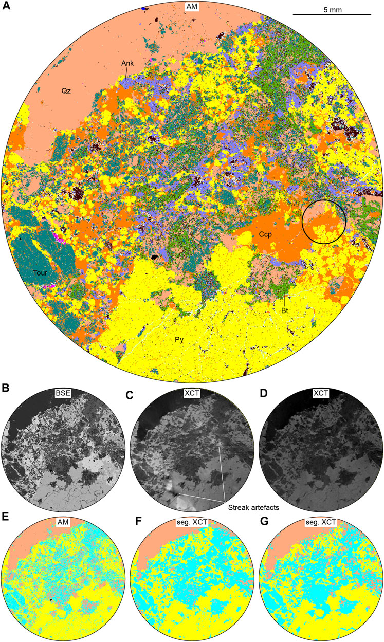
FIGURE 5. AM and XCT images of a polished rock chip of a mineralized quartz-(tourmaline-calcite) vein (sample 2). For color coding of the minerals, see Table 2. (A) 30 μm pixel size AM mineral map. The black circle indicates the overlapping region between the 1 μm pixel size AM mineral map and the 4 μm voxel size XCT scan (see Figure 6). (B) 1.87 μm AM BSE image. (C) 30 μm voxel size XCT scan. The image displays some bright and dark spots, streak artefacts from scheelite in the rock chip of sample 1 because of stacking of the samples for XCT analysis. (D) 45 μm voxel size XCT scan. (E) Simplified 30 μm pixel size AM mineral map. (F) 30 μm voxel size segmented XCT scan. (G) 45 μm voxel size segmented XCT scan. Abbreviations: Ank – ankerite, Bt – biotite, Ccp – chalcopyrite, Py – pyrite, Tour – tourmaline, Qz – quartz.

In a small area within the AM mineral map, two pixels are identified as Au: one in pyrite, the other in adjacent quartz. This region of interest was subsequently scanned by AM at 1 μm pixel size (Figures 5, 6). It reveals numerous <30 μm Au grains (and Ag, Bi) within the pyrite and quartz, but also tourmaline, ankerite, and chlorite (Figure 6). Similarly, the XCT scan at 4 μm voxel size of the mini core, drilled through this region of interest, shows many more dense particles not seen in the coarser scans (Figure 4). Yet, the Au grains identified by AM are not resolved. The smaller size of the mini core compared with the rock chip allows XCT analysis at lower beam energy (80 kV), which makes visual separation of chalcopyrite and pyrite possible (Figure 6). Yet, grey levels are still too close for meaningful histographic segmentation. The change in beam energy also causes tourmaline to dominantly be classified together with quartz rather than the group of silicates/carbonates. Table 3 summarizes the quantitative comparison of this region of interest between the 1 μm pixel size AM scan and all other scans. Expectedly, but still noteworthy, the detection of heavy minerals is higher for AM than XCT and increases with scan resolution for both techniques. The detected amounts for silicates/carbonates and quartz/albite vary significantly, partly due to the change in beam energy (160–80 kV) for XCT analysis and in consequence ambiguous classification of some minerals (e.g., tourmaline). Yet again, overall detection of heavy minerals (all slices) is much higher for XCT than AM (Figure 4). For the 4 μm voxel size XCT scan, the portion of the class of heavy minerals in the top XCT slice is only 0.01% of the volume across all slices.

FIGURE 6

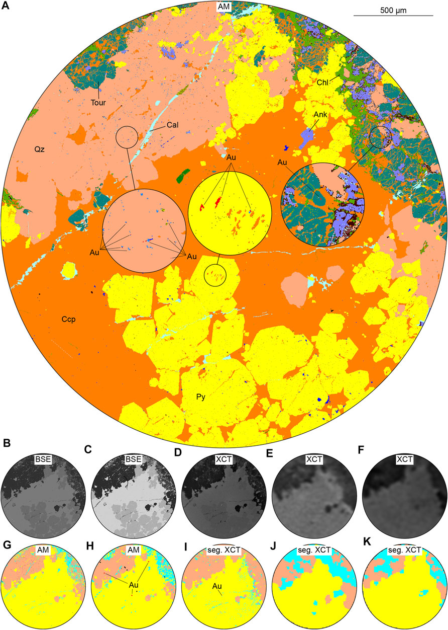
FIGURE 6. AM and XCT images of a region of interest in the polished rock chip of sample 2. For color coding of the minerals, see Table 2. (A) 1 μm pixel size AM mineral map. The circles show enlarged images of the small circles. Gold inclusions are found in a number of minerals but are very fine-grained. The marked grains represent only a portion of the Au grains detected in the map. (B) 1.87 μm pixel size AM BSE image. (C) 250 nm pixel size AM BSE image. (D) 4 μm voxel size XCT scan. (E) 30 μm voxel size XCT scan. (F) 45 μm voxel size XCT scan. (G) 1 μm pixel size simplified AM mineral map. The same gold grains as in (A) are detected but not visible in the map due to the small size of the image. (H) 30 μm pixel size simplified AM mineral map. Three Au grains are detected. (I) 4 μm voxel size segmented XCT scan. One Au grain is detected. (J) 30 μm voxel size segmented XCT scan. (K) 45 μm voxel size segmented XCT scan. The loss in detail between the 4 μm XCT scan (D, I) and the 30 μm (E, J) and 45 μm (F, K) XCT scans is apparent. Abbreviations: Ank – ankerite, Cal – calcite, Ccp – chalcopyrite, Chl – chlorite, Py – pyrite, Tour – tourmaline, Qz – quartz.

The 1 μm voxel size XCT scan of a cylindrical volume (1 mm height, 1 mm diameter) within the mini core was centered around the largest Au grain in pyrite (identified by AM). This scan resolves the Au grain and many more dense particles with depth, undetected by the 4 μm voxel size scan (Figure 4). Conversely, visual separation between chalcopyrite and pyrite is not possible. The position of the cylinder within the mini core causes the mini core to act as a shield against the x-rays. Hence, a high beam energy (160 kV) is necessary for proper x-ray penetration.

The study of this sample demonstrates how information on the occurrence and distribution of particularly fine-grained minerals, such as heavy trace metal minerals, is highly reliant on the technique and resolution of analysis.

Molybdenite- and Scheelite-Bearing Quartz Veins in Aplite (Sample 3)

The AM mineral map shows the aplite dyke to consist mainly of K-feldspar, plagioclase, and quartz with minor biotite and muscovite (Figure 7). Sulfides (pyrite, pyrrhotite, and chalcopyrite), tourmaline, and calcite occur disseminated. In the sample, three quartz vein connect at an angle (Figure 7). Molybdenite mineralization occurs in one vein but not in the others. Conversely, scheelite occurs in one of the other veins but not in the molybdenite-filled vein. Chalcopyrite, pyrite, and pyrrhotite are found in all three veins. In the XCT data, differentiation of the aplite dyke is hardly possible due to beam hardening correction optimized for the highly attenuating scheelite and molybdenite rather than the silicates and carbonates (similar to sample 1). Only the disseminated sulfides can be segmented from the silicates. Yet, comparison between the mineral map and the top slice of the XCT data show a considerable under-segmentation of sulfides and over-segmentation of silicates (Figure 7, Table 4). Nevertheless, the veins and their orientation in the sample are clearly visible. XCT data confirms the separation of scheelite and molybdenite into two veins and shows the extent of the mineralization with depth in the sample (Figure 8). XCT also shows that the veins are dipping in the same direction. In addition, individual segmentation of both scheelite and molybdenite is possible and the quantitative difference between AM and XCT is similar for both minerals (Table 4). The main errors for scheelite come from streak artefacts and a pronounced partial volume effect at grain boundaries (despite the use of a Sobel filter) in the XCT data. For molybdenite, errors are especially miss-segmentation of fine grains as silicates and sulfides. This is because blurring is more pronounced in fine molybdenite grains (Hanna and Ketcham 2017), which therefore appear darker than larger molybdenite grains in the XCT images.

FIGURE 7

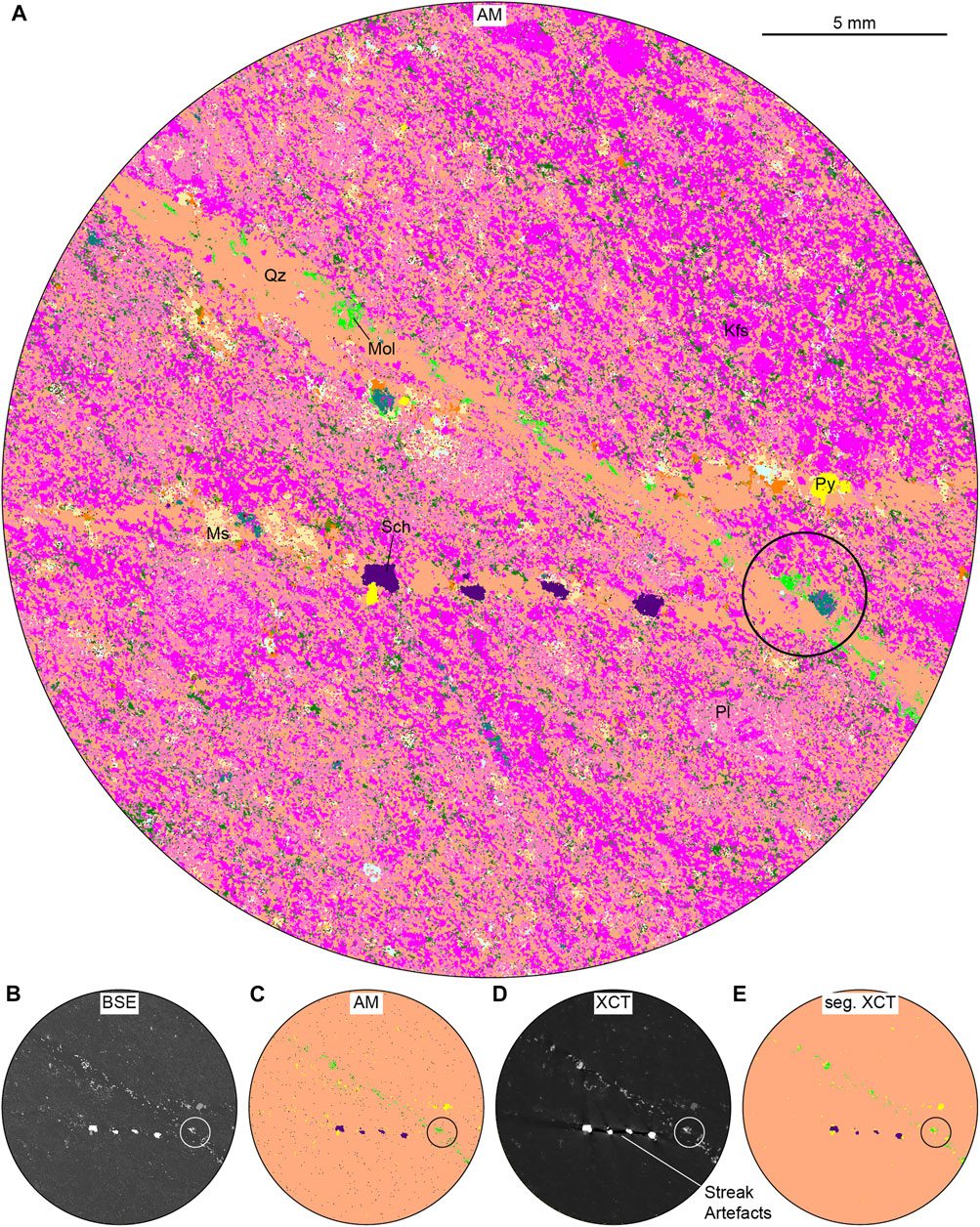
FIGURE 7. AM and XCT images of a polished rock chip of scheelite- and molybdenite-mineralized quartz veins in an aplite dyke (sample 3). For color coding of the minerals, see Table 2. (A) 30 μm pixel size AM mineral map. The black circle indicates the overlapping region between the 1 μm pixel size AM mineral map and the 4 μm voxel size XCT scan (see Figure 9). (B) 1.87 μm pixel size AM BSE image. (C) 30 μm pixel size simplified AM mineral map. (D) 30 μm voxel size XCT scan. The scheelite grains cause some streak artefacts. (E) 30 μm voxel size segmented XCT scan. Some of the silicates/carbonates in contact with scheelite are segmented as sulfides/oxides due to the streak artefacts but overall impact is minor. Abbreviations: Kfs – k-feldspar, Mol – molybdenite, Ms – muscovite, Pl – plagioclase, Py – pyrite, Sch – scheelite, Qz – quartz.

TABLE 4

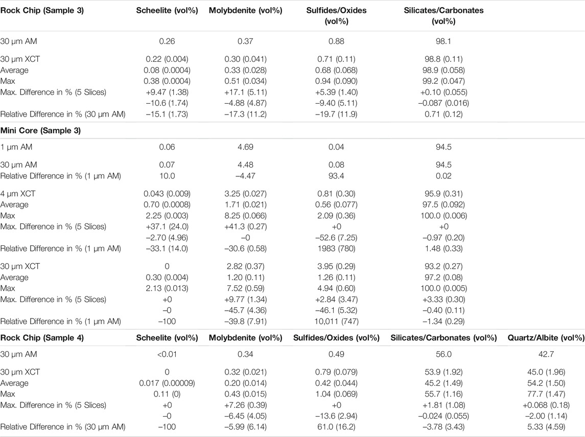
TABLE 4. Comparison of the area percentage of the classes segmented in the rock chip and mini core of samples 3 and 4 between the AM mineral maps and the corresponding slice of the different XCT scans. Additionally, the maximal difference in percent between the XCT slice used for comparison with AM and the following four slices is shown. Average and Max values refer to all slices within a specific segmented volume (rock chip, mini core) of an XCT data set. The XCT values are the mean values of six segmentations (n = 6) of the same volume, with the standard deviation in brackets.

FIGURE 8

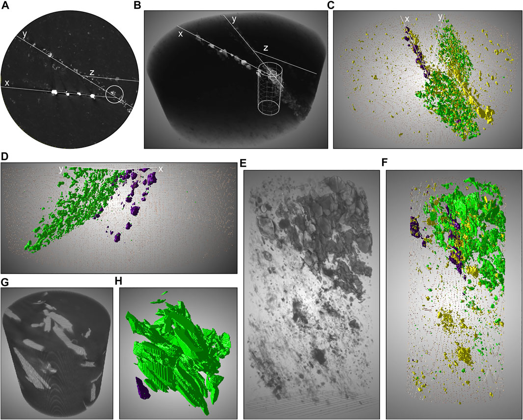
FIGURE 8. XCT images of the rock chip and mini core of sample 3. For color coding of the minerals, see Table 2. (A) Top slice of the sample showing quartz veins with mineralization of scheelite (x), molybdenite (y), and sulfides (z) in an aplite dyke. (B) 3D-rendered XCT image (30 μm voxel size) of the rock chip. The white cylinders indicate the position of the mini core and the subvolume within. (C) 3D segmented volumes of scheelite, molybdenite, and sulfides. All veins dip to the right and show mineralization extending with depth in the sample. (D) Different view of (C) without the sulfides. The control of the veins on mineralization and the contact between the veins are clearly displayed. (E) 3D-rendered XCT image (4 μm voxel size) of the mini core (stripped of silicates/carbonates). (F) 3D segmented volumes of scheelite, molybdenite, and sulfides in the mini core. Sulfides in the upper, molybdenite-dominated part are mostly wrongly segmented molybdenite grains. (G) 3D-rendered XCT subvolume (1 μm voxel size) within the mini core. (H) 3D segmented volumes of scheelite and molybdenite in the subvolume of the mini core. The molybdenite grains are flaky but aligned with the vein. Hence, grains appear as thin and elongated in the 2D sections.

The 1 μm pixel size scan by AM was focused on an area of molybdenite mineralization at the intersection of the molybdenite-bearing quartz vein with the scheelite-bearing quartz vein. In several molybdenite grains, bright inclusions (a few micron large) are visible in the BSE image (Figure 9). Some grains are identified as hessite associated with native Bi, others escape detection. The topography of many deformed and fractured molybdenite grains is particularly problematic. Uneven surfaces cause low and spurious x-ray counts in the EDS detector (Newbury and Ritchie 2015). To limit misidentification a cut-off value was set at 1,000 x-ray counts per pixel. As a result, many molybdenite grains contain unclassified areas (Figure 9). At the intersection between the quartz veins, three (∼40–80 μm) large scheelite grains were detected, but well separated from the molybdenite grains. The XCT data reveal the contact between scheelite and molybdenite mineralization at depth in the sample, but are unsuccessful in resolving heavy mineral inclusions in molybdenite (Figure 8). Streak artefacts and blurring of the scheelite and molybdenite grains affect segmentation of the XCT data. Particularly, grain edges and space between grains in clusters of molybdenite grains are segmented as sulfides due to blurring of bright molybdenite with dark quartz. This causes an extreme over-segmentation of sulfides compared to AM and shows why for example AM is needed to correctly interpret XCT data (Table 4).

FIGURE 9

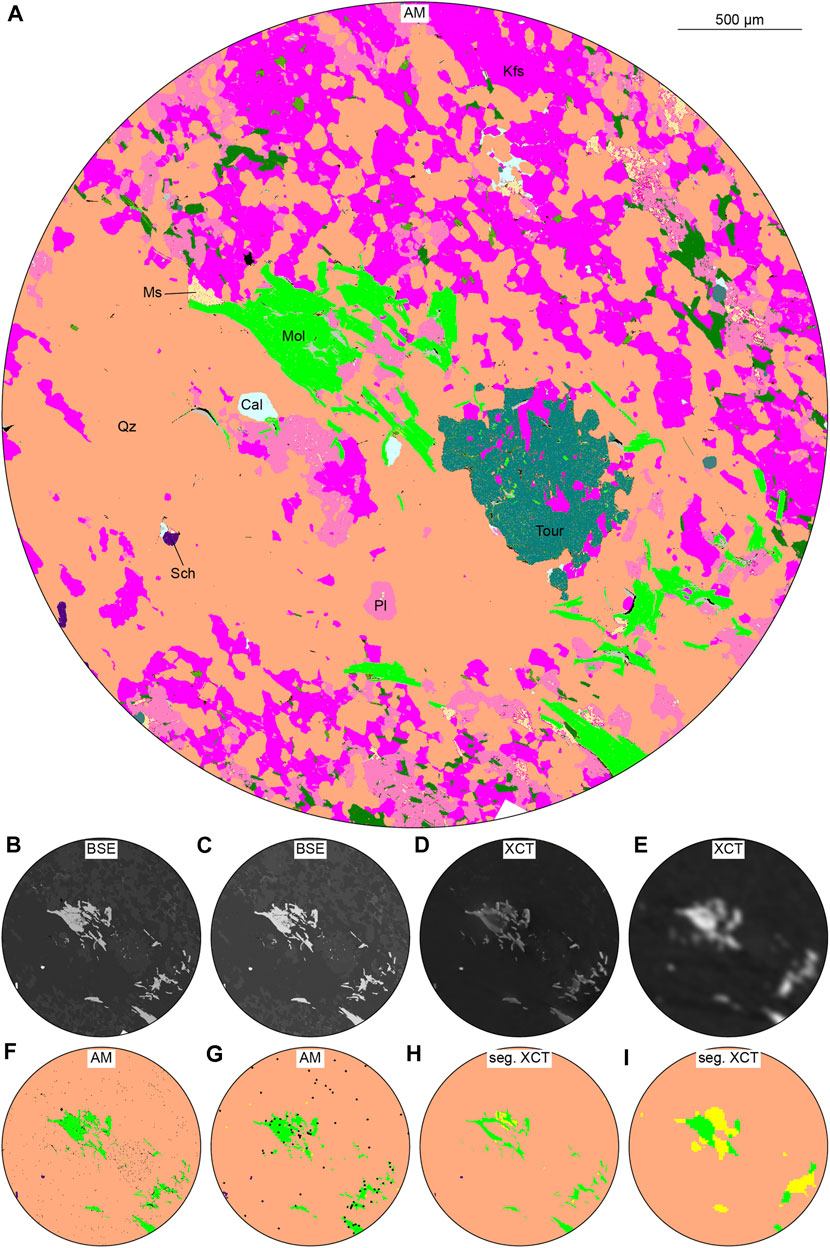
FIGURE 9. AM and XCT images of a region of interest in the polished rock chip of sample 3. For color coding of the minerals, see Table 2. (A) 1 μm pixel size AM mineral map. Uneven topography in some molybdenite grains caused issues with EDS analysis, rendering some areas in the molybdenite grains unclassified. (B) 250 nm pixel size AM BSE image. (C) 1.87 μm pixel size AM BSE image. (D) 4 μm voxel size XCT scan. (E) 30 μm voxel size XCT scan. (F) 1 μm pixel size simplified AM mineral map. (G) 30 μm pixel size simplified AM mineral map. (H) 4 μm voxel size segmented XCT scan. (I) 30 μm voxel size segmented XCT scan. Abbreviations: Cal – calcite, Kfs – k-feldspar, Mol – molybdenite, Ms – muscovite, Pl – plagioclase, Sch – scheelite, Tour – tourmaline, Qz – quartz.

The XCT scan (cylinder with 1 mm height and diameter) of 1 μm voxel size of a molybdenite cluster is still hardly of good enough quality to resolve heavy mineral inclusions. Yet their presence in molybdenite of the Liikavaara Östra Cu-(W-Au) deposit is known from AM and prior studies by synchrotron radiation x-ray fluorescence mapping (Warlo et al. submitted). The study of such small-scale features might be difficult to achieve in a lab and could require e.g., synchrotron-based XCT (Wang and Miller 2020). Nevertheless, the high-resolution XCT scan successfully visualizes the flaky texture of molybdenite well (Figure 8). All three XCT scans show molybdenite grains to be predominantly aligned with the vein (Figure 8). For that reason, many molybdenite grains in the surface maps appear as thin elongated grains (cut more or less perpendicular to the crystallographic c-axis) rather than tabular flakes.

Molybdenite-Rich Contact Between a Quartz Vein and Biotite Schist (Sample 4)

AM analysis shows gradually increasing biotitization of the K-feldspar and plagioclase matrix of the biotite schist towards the contact with the quartz vein (Figure 10). It also reveals ubiquitous epidote and tourmaline alteration within the biotite schist. The quartz vein contains disseminated calcite, which extends into the biotite schist. A thin straight calcite veinlet cuts through the quartz vein and continues as a zigzagging chlorite veinlet through the biotite schist. It also cuts disseminated pyrite associated with chalcopyrite (Figure 10). Mineralization of pyrite, chalcopyrite, pyrrhotite, and sphalerite within the quartz vein is strongly associated with calcite, which appears to replace the sulfides. Molybdenite mainly occurs along the contact of the quartz vein with the biotite schist and shows association with calcite but no signs of replacement like the other sulfides. Finally, a single rounded 100 μm large grain of scheelite is found in the quartz vein. In the XCT data, low or missing contrast in the grey values between many minerals results in a very simplified segmentation of five mineral classes (Figure 10, Table 4): 1) quartz and albite, 2) silicates and carbonates, 3) sulfides and oxides, 4) molybdenite, and 5) scheelite. This means that most of the features observed by AM concerning the biotite schist cannot be differentiated by XCT (Figure 10). In addition, calcite dissemination within the quartz vein is poorly resolved. However, it is possible to follow the molybdenite mineralization towards depth in the sample along the contact between the quartz vein and biotite schist (Figure 11). Additionally, larger scheelite grains are revealed at depth in the sample (Figure 11). Comparison of the top sample slice with AM shows a relatively good fit of segmented molybdenite, whereas sulfides/oxides are over-segmented (Table 4). Under-segmentation of silicates/carbonates appears to compensate mainly for this difference (Table 4). The scheelite grain observed by AM is too fine-grained for proper resolution and segmented as quartz/albite.

FIGURE 10

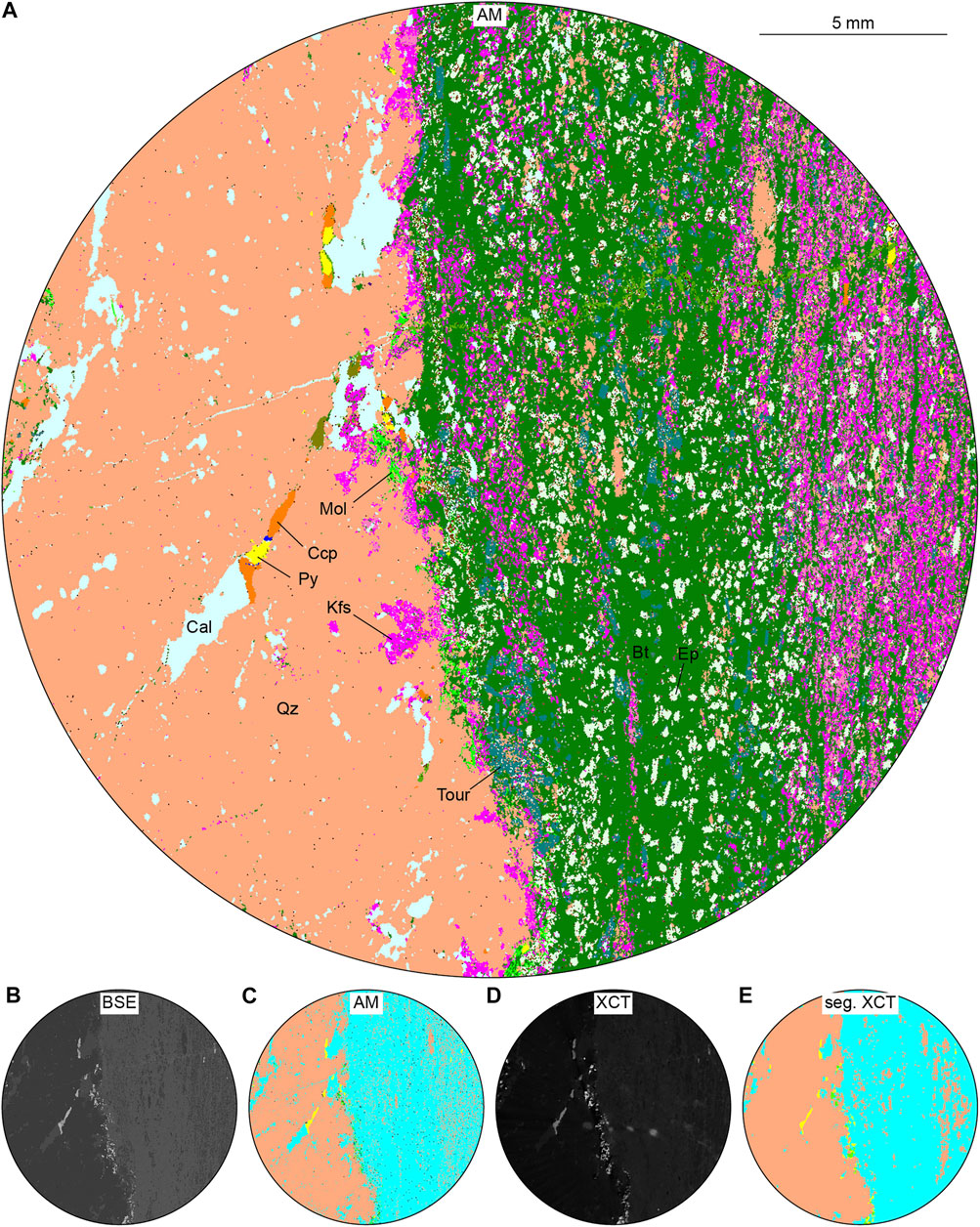
FIGURE 10. AM and XCT images of a polished rock chip of molybdenite mineralization along the contact between a quartz vein and biotite schist (sample 4). For color coding of the minerals, see Table 2. (A) 30 μm pixel size AM mineral map. (B) 1.87 μm pixel size AM BSE image. (C) 30 μm pixel size simplified AM mineral map. (D) 30 μm voxel size XCT scan. (E) 30 μm voxel size segmented XCT scan. Abbreviations: Bt – biotite, Cal – calcite, Ccp – chalcopyrite, Ep – epidote, Kfs – k-feldspar, Mol – molybdenite, Py – pyrite, Tour – tourmaline, Qz – quartz.

FIGURE 11

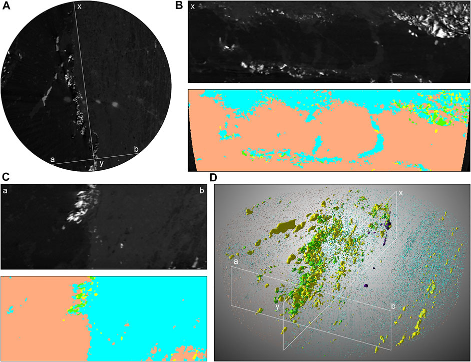
FIGURE 11. XCT images of the rock chip of sample 4. For color coding of the minerals, see Table 2. (A) Top slice showing the position of two profiles seen in (B,C). (B) Profile along the contact between the quartz vein and biotite schist. X-ray attenuation image (top) and segmented image (bottom). (C) Profile across the contact between the quartz vein and biotite schist. X-ray attenuation image (top) and segmented image (bottom). (D) 3D segmented volumes of molybdenite and sulfides. Volumes of silicates/carbonates and quartz/albite are indicated by dots.

Discussion

The results reveal several challenges with the correlation and integration of AM and XCT data. Yet they also show how multi-scale analysis of AM and XCT may aid in ore characterization. Below both aspects are discussed.

Correlation and Integration of Automated Mineralogy and X-Ray Computed Tomography Data

Linking AM and XCT has a strong potential in (ore) geology to improve quantitative and textural information on a rock sample (Butcher 2020). XCT is already applied in combination with x-ray diffraction microtomography (e.g., Artioli et al., 2010; Valentini et al., 2011; Mürer et al., 2018; Takahashi and Sugiyama 2019) and x-ray fluorescence microtomography (e.g., Wildenschild and Sheppard 2013; Laforce et al., 2017; Suuronen and Sayab 2018), although mainly constrained to synchrotron facilities and very small sample sizes. In contrast, the recently developed Oreexplore GeoCore X10 merges XCT with x-ray fluorescence analysis for drill core pieces up to 4 × 1 m but limited to a maximal voxel size of 200 μm (Bergqvist et al., 2019). The combination of these analytical techniques in a single system is possible since all techniques utilize an x-ray beam. In contrast, AM is an electron beam-based technique. Thus, a combination of XCT and AM in a single system is impossible with the current technological knowledge. Instead, research and development have to focus on software solutions to improve cross-system integration. So far commercially available integration of XCT and AM only concerns geo-referencing of samples for easier visual correlation and presentation (e.g., Zeiss Atlas 5). This is mainly helpful for qualitative comparison, e.g., for the XCT data to aid in 3D interpretations of AM data. In this study, XCT scans of ore samples show the extent of mineralization with depth in the samples, the angle and orientation of veins, and shapes and sizes of well-separated mineral grains of high contrast to the surrounding phases (e.g., molybdenite, scheelite, heavy minerals). Yet, the segmentation and study of gangue minerals like silicates and carbonates in XCT datasets is challenging, due to too low grey value contrast between the minerals. While in this study AM analysis was mainly performed prior to XCT analysis, results suggest XCT also to be useful for targeted sampling for 2D analysis. In none of the XCT analyses, the topmost slice (the polished surface, which was also analyzed by AM) is the slice with the highest content of the minerals of interest (heavy minerals, molybdenite, and scheelite; Tables 3, 4). Hence, if the goal was to maximize the amount of these minerals in a sample for AM, the XCT scan data should be used to guide the sub-sampling of the sample. This would be especially helpful to better quantify trace metal minerals, as the required number of grains for statistical robustness could be achieved with fewer samples (Goodall and Scales 2007; Godel 2013).

On the other hand, integrating 2-dimensional AM data and 3-dimensional XCT data for quantitative analysis is not straightforward. The reliance on dedicated software to process 2-dimensional AM data is a challenge when merging with 3-dimensional XCT data. The AM software used in this study (Mineralogic Explorer) calculates valuable mineral parameters like mineral association, grain size distribution, metal deportment, etc. but only for the entire AM scan. Obtaining this information for a region of interest in the scan, e.g., for better fitting with the XCT data, is not possible. Further, the software is limited to the processing of AM data. AM and XCT images are easily overlaid in a graphical software but at the cost of losing the functionalities of the AM software. In addition, success in overlaying the images can depend on the quality of the stitching of the montaged AM mineral map. In this study, multiple steps were required to integrate the AM mineral maps into the XCT processing software (ORS Dragonfly) for geo-referencing and quantitative analysis. Currently, the best way to address data integration between AM and XCT seems to be through programming of dedicated algorithms in e.g., MatLab (Reyes et al., 2017; Guntoro et al., 2019b). However, this requires proficiency in programming. Furthermore, software is not the only challenge concerning quantitative correlation.

In this study, one issue of XCT analysis was x-ray attenuation artefacts at the top of the samples (cone-beam effect; Cnudde and Boone 2013). To prevent these artefacts, the epoxy mounted rock samples were stacked with their surfaces facing each other during XCT analysis. However, instead dense minerals caused artefacts into adjacent samples. Thus, to resolve this issue the topmost slices were excluded from segmentation. Consequently, comparison with AM of the same exact surface was hardly possible. To assess the impact of a potential slight vertical offset between the AM mineral maps and topmost segmented XCT slices on quantitative comparison, the relative variation in bulk mineralogy across the five topmost segmented XCT slices was calculated in all scans (Tables 3, 4). Results indicate that the variation in bulk mineralogy is generally smaller between XCT slices than between AM and XCT for major and minor phases. This is to say, segmentation plays a larger role in the quantitative differences between AM and XCT than a potential vertical offset. Yet, for trace phases, especially the heavy mineral phase in sample 2, variation between slices is larger than between AM and XCT. This is due to the small grain size of the heavy minerals, which are partly not detectable across more than one slice. To improve correlation a better approach may be to cut and polish a rock sample after XCT analysis, to perform AM on a surface corresponding to an inner slice in the XCT data, unaffected by the cone-beam effect. An even better alternative may be to try to remove the cone-beam effect altogether. This is achieved with a helical scanning trajectory (De Witte 2010; Cnudde and Boone 2013) or a multiscan with top and bottom scans centered on the edges of the sample.

A 30 μm step size was chosen for both AM and XCT analysis for better modal comparison. Yet, effective resolution differed significantly. For AM, a 30 μm pixel size was sufficiently large not to cause overlap of the beam interaction volume with more than one pixel. In contrast, in XCT analysis the impact of mineral grains on the calculated x-ray linear attenuation exceeded their own voxels due to instrument-related resolution limitations (Kyle and Ketcham 2015; Hanna and Ketcham 2017). This blurring resulted in a relatively worse resolution of XCT than AM. To achieve similar resolution, a better XCT instrument would need to be used and/or the step size of XCT analysis reduced. Yet, the latter would entail a reduction in scanning volume also (Kyle and Ketcham 2015). Moreover, other artefacts like beam hardening, particularly for high-Z mineral grains, would persist (Kyle and Ketcham 2015). Hence, a perfect correlation of XCT data with AM data is hardly possible.

The possibility to differentiate between individual minerals is much lower for XCT than AM due to the nature of the techniques (x-ray linear attenuation coefficients vs. energy dispersive x-ray spectra coupled with backscattered electron intensity). Thus, AM mineral maps require simplification for correlation with the segmented mineral classes of XCT. This simplification may be based on visual comparison of the data sets and calculations on the x-ray linear attenuation coefficients for the various minerals quantified by AM. The approach works well for coarse-grained minerals, easily identified in the data of both techniques, but is less reliable for fine-grained minerals, which are blurred and lack distinct grain boundaries in the XCT images. Furthermore, in this study, molybdenite grains are significantly darker than scheelite grains in all analyses of this study, regardless of size and shape, despite a higher calculated x-ray linear attenuation coefficient. This creates ambiguity regarding which segmented class some minerals belong to.

Reliable mineral segmentation of XCT data, particularly of complex geological samples, is challenging, as described in literature (e.g., Godel 2013; Guntoro et al., 2019a, 2019b; Wang and Miller 2020), but also demonstrated by the results of this study. The challenge starts with the generation of high-quality images used for segmentation: 1) the co-occurrence of minerals with largely different x-ray linear attenuation coefficients makes choosing a beam energy optimized to separation of all minerals impossible. The same applies to selecting of filters and beam hardening corrections post analysis (Herman 1979; Kyle and Ketcham 2015; Hanna and Ketcham 2017). Rocks abundant in heavy minerals require high beam energies for adequate x-ray penetration. This lowers the x-ray attenuation contrast between many minerals. In addition, analytical settings to minimize streak artefacts of highly attenuating minerals like scheelite lower overall beam intensity, thus requiring longer scan times (Gusenbauer et al., 2016). Post-analysis metal artefact reduction methods exist but are not yet common in industrial XCT analysis (Gusenbauer et al., 2016). Combining the results from multiple scans at varied beam energies may help to alleviate some of the issue concerning the x-ray linear attenuation coefficient but comes with a cost of increased scan time. 2) Choosing a voxel size to resolve features of interest adequately while minimizing scan time (and thereby cost of analysis) is difficult in rocks of heterogeneous grain size. Fine intergrowths of minerals with small differences in attenuation coefficient easily become visually homogenized through blurring. A small voxel size may not be cost effective due to long scan times, but too large a voxel size carries the risk of small grains to be unresolved. Additionally, scan volume limits the available scan resolution (Kyle and Ketcham 2015). 3) The edge contrast between mineral grains, especially for minerals of similar x-ray attenuation coefficient (e.g., silicates), is less pronounced than between e.g., grain and air, which makes segmentation more difficult in low-porosity rocks. 4) Minerals may exhibit a large range of grey scale values, even if chemical composition is uniform, based on grain size and associated minerals due to blurring (Kyle and Ketcham 2015). Other artificial grey scale variations (e.g., gradients, partial volumes, streaks, shadows, and rings) cause overlap in the grey scale value ranges of minerals of similar x-ray linear attenuation coefficient, which again constrains segmentation.

Recently, advancements have been made to improve segmentation of XCT data through matching of slices in the XCT data with corresponding AM quantitative maps via a MatLab algorithm, which are then used to determine global thresholds for segmentation (Reyes et al., 2017) or as training data for machine learning algorithms (Guntoro et al., 2019b; Guntoro et al., 2020). Results were shown to be superior to traditional segmentation techniques like grey scale thresholding or watershed segmentation (Reyes et al., 2017; Guntoro et al., 2019b). This integration of XCT and AM is promising and will perhaps help to routinize the use of XCT in ore geology and the mining industry in the future. However, the complexity of the method, the necessity of proficient programming skills, and a relatively long post-processing time per sample are still an obstacle to broad application. In this study, especially the segmentation of chalcopyrite and pyrite in the XCT scan of the mini core of sample 2 and molybdenite in the rock chips of samples 3 and 4 could benefit from the use of machine learning. Concerning chalcopyrite and pyrite, they are clearly differentiable with the naked eye in the 80 kV scan, yet histographic segmentation is unsatisfactory (Figure 6). The slight grey scale gradient from the center to the sidewalls of the cylinder causes overlap of grey scale values between the minerals (cupping effect; Cnudde and Boone 2013). Additionally, the noise in the images prevents the sobel filter from properly resolving grain boundaries between pyrite and chalcopyrite despite sharpening and denoising of the XCT images. Matching of the characteristic cubic shaped pyrite grains between the XCT data and AM may however overcome these hurdles. Similarly, molybdenite grains have rather distinct elongated shapes, which may support discrimination against other sulfides of similar x-ray linear attenuation coefficient. In this study, especially the decrease in brightness of molybdenite with grain size leads to false segmentation of small molybdenite grains as sulfides/oxides and silicates/carbonates.

Multi-Scale Analysis

For every type of microanalysis method, time-to-result (and therefore the cost), has to be weighed up against the resolution needed to resolve the textures and mineral chemistry, which in turn may impact the quantity and quality of information gained. As a consequence, a common approach is sequential analysis – where the resolution is increased but at the same time the area scanned is made progressively smaller. This approach of ‘zooming in’ on a region of interest was also used in this study.

In the 30 μm pixel size AM mineral map of the rock chip of sample 2, several Au and Ag minerals are detected, but generally not in sizes larger than 1 or 2 pixels (Figure 5). The subsequent 1 μm pixel size scan on a much smaller area reveals numerous grains of Au, Ag, and Bi that are undetected in the 30 μm resolution scan (Figure 6). Thus, the 1 μm resolution provides much better information on parameters like grain size distribution, mineral association, etc. Obviously, a 1 μm pixel size scan of the entire polished surface of the rock chip would be ideal, yet it would consume an unreasonable amount of time (several days) to complete. In addition, if and to what extend identification of trace metal minerals could be expected would be purely based on observations of e.g., petrographic microscopy (often too low resolution) or manual SEM-EDS (mainly spot-checking, possibly time-consuming). Hence, the coarser but faster 30 μm scan serves as a good overview and allows targeted high-resolution analysis. Similar results are obtained by XCT, where with each scan at a smaller voxel size heavy mineral grains that the prior scans fail to resolve are detected (Figures 4, 6). Generally, coarser grains account for the majority of the bulk metal in an ore deposit and fine grains, even in high numbers, accumulate to only a small overall volume. In mining, loss of the finest-grained fractions is commonly accepted, partly due to missing tools and added costs for their recovery. However, for economic trace metals like Au, the fine-grained fractions can be substantial and loss to tailings a significant loss in potential profit (Vaughan 2004). Hence, these high-resolution analyses are needed to provide the necessary knowledge to develop production strategies.

Similarly, the study of molybdenite grains in the rock chip and mini core of sample 3 shows how high-resolution analyses are necessary to quantify micro- and nano-inclusions in molybdenite grains. Even the 1 μm resolution scans of AM and XCT only managed to resolve a small portion of the inclusions. Although the effect of these inclusions on processing of molybdenite requires more research, a study by Triffett et al. (2008) suggests foreign mineral grains trapped in molybdenite have potentially a negative effect on flotation.

Conclusion

XCT can aid AM in various ways: 1) The technique is well suited to provide three-dimensional visualization of textures and structures at centimeter-to micron-scale. The separation of molybdenite and scheelite mineralization onto two different quartz veins observed by AM in this study was confirmed to extend with depth in the sample. Furthermore, the XCT data revealed similar dipping angles and dip directions for the two quartz veins. In contrast, the seemingly straight contact between a quartz vein and biotite schist observed by AM was shown to be more rugged with depth by XCT. 2) XCT can help assess the stereological error of 2D analysis, although in this study it was limited to qualitative assessment of only well-separated high-contrast grains (e.g., Bi-minerals and scheelite). The stereological error was not quantified as no proper grain separation of the segmented XCT data was performed, e.g. molybdenite clusters were registered as a single grain rather than an accumulation of grains. Grain separation is possible but very time consuming and was not the focus of this study. 3) XCT can increase data volume on rare minerals to quickly achieve statistical robustness and guide (sub)-sample selection. In this study, heavy trace minerals in a single XCT slice constituted only a tiny fraction of the amount of heavy trace minerals within the entire volume of an XCT scan. Furthermore, the XCT slice corresponding to an AM mineral map was never the slice with the highest amount of heavy trace minerals. 4) XCT can be performed at various scales and allows zooming in onto an area of interest. In this study, successive sub-sampling (by e.g., mini-coring) allowed XCT analysis of a 1 × 1 mm cylindrical volume at 1 μm voxel size from within a ∼20 cm long drill core piece, previously scanned at 45 μm voxel size. Further, despite the destruction caused by the sub-sampling, the spatial information of the rock samples was preserved in the XCT data to allow interpretation of the data in its original spatial context.

AM, on the other hand, can also guide subsampling for high-resolution XCT (e.g., drilling of mini cores) and help with the segmentation of the XCT data. Yet, quantitative integration of XCT and AM data remains challenging and is restricted by the quality of segmentation of the XCT data. This is particularly true for low-porosity rock samples with complex mineralogy like in this study. Despite this, recent studies look promising for improving segmentation and thereby gaining more quantitative mineral analysis of XCT data. Overall, linking XCT and AM provides a better characterization of an ore than applying only one technique, or using them separately (Warlo et al., Forthcoming 2021).

Data Availability Statement

The raw data supporting the conclusions of this article will be made available by the authors, without undue reservation.

Author Contributions

MW, AB, GB, and CW designed the study. MW collected the samples for analysis and performed the mini drilling. MW performed the Automated Mineralogy analysis including processing of the data. JK did the x-ray computed tomography analysis at the Geological Survey of Finland including corrections to the data post analysis. FF and HL performed the x-ray computed tomography analysis at Luleå University of Technology and also corrected the data post analysis. MW processed and segmented the x-ray computed tomography data in Dragonfly and did the correlation with the Automated Mineralogy data. MW compiled the results and wrote the manuscript. GB, CW, AB, JK, FF, and HL provided feedback to the manuscript.

Funding

This study was funded by the Center of Advanced Mining and Metallurgy (CAMM) at Luleå University of Technology, together with Boliden Mineral AB. XCT at the Geological Survey of Finland was funded by the Academy of Finland through the RAMI infrastructure grant (#293109).

Conflict of Interest

The authors declare that the research was conducted in the absence of any commercial or financial relationships that could be construed as a potential conflict of interest.

Publisher’s Note

All claims expressed in this article are solely those of the authors and do not necessarily represent those of their affiliated organizations, or those of the publisher, the editors and the reviewers. Any product that may be evaluated in this article, or claim that may be made by its manufacturer, is not guaranteed or endorsed by the publisher.

Acknowledgments

Ignacio Gonzalez-Alvarez is thanked for constructive editorial work and three reviewers for significantly improving the manuscript. The authors would also like to thank Boliden Mineral AB for permitting the study on rock samples of the Liikavaara Östra Cu-(W-Au) deposit. An earlier version of this manuscript has previously appeared in the doctoral thesis by Warlo (2021).

Supplementary Material

The Supplementary Material for this article can be found online at: https://www.frontiersin.org/articles/10.3389/feart.2021.789372/full#supplementary-material

References

Artioli, G., Cerulli, T., Cruciani, G., Dalconi, M. C., Ferrari, G., Parisatto, M., et al. (2010). X-ray Diffraction Microtomography (XRD-CT), a Novel Tool for Non-invasive Mapping of Phase Development in Cement Materials. Anal. Bioanal. Chem. 397 (6), 2131–2136. doi:10.1007/s00216-010-3649-0

PubMed Abstract | CrossRef Full Text | Google Scholar

Baker, D. R., Mancini, L., Polacci, M., Higgins, M. D., Gualda, G. A. R., Hill, R. J., et al. (2012). An Introduction to the Application of X-ray Microtomography to the Three-Dimensional Study of Igneous Rocks. Lithos 148, 262–276. doi:10.1016/j.lithos.2012.06.008

CrossRef Full Text | Google Scholar

Bam, L., Miller, J., and Becker, M. (2020). A Mineral X-ray Linear Attenuation Coefficient Tool (MXLAC) to Assess Mineralogical Differentiation for X-ray Computed Tomography Scanning. Minerals 10 (5), 441. doi:10.3390/min10050441

CrossRef Full Text | Google Scholar

Berger, M. J., Hubbell, J. H., Seltzer, S. M., Chang, J., Coursey, J. S., Sukumar, R., et al. (2010). XCOM: Photon Cross Sections Database. NIST Stand. Reference Database 8 (XGAM), NBSIR 87–3597. doi:10.18434/T48G6X

CrossRef Full Text | Google Scholar

Bergqvist, M., Landström, E., Landström, E., and Luth, S. (2019). Access to Geological Structures, Density, Minerals and Textures through Novel Combination of 3D Tomography, XRF and Sample Weight. ASEG Extended Abstr. 2019 (1), 1–3. doi:10.1080/22020586.2019.12073146

CrossRef Full Text | Google Scholar

Butcher, A. R. (2020). Upscaling of 2D Mineralogical Information to 3D Volumes for Geoscience Applications Using a Multi-Scale, Multi-Modal and Multi-Dimensional Approach. IOP Conf. Ser. Mater. Sci. Eng. 891 (1), 012006. doi:10.1088/1757-899X/891/1/012006

CrossRef Full Text | Google Scholar

Cnudde, V., and Boone, M. N. (2013). High-resolution X-ray Computed Tomography in Geosciences: A Review of the Current Technology and Applications. Earth-Science Rev. 123, 1–17. doi:10.1016/j.earscirev.2013.04.003

CrossRef Full Text | Google Scholar

De Man, B., Nuyts, J., Dupont, P., Marchal, G., and Suetens, P. (1998). Metal Streak Artifacts in X-ray Computed Tomography: a Simulation Study. IEEE Nucl. Sci. Symp. Conf. Rec. 3, 1860–1865. doi:10.1109/NSSMIC.1998.773898

CrossRef Full Text | Google Scholar

De Witte, Y. (2010). Improved and Practically Feasible Reconstruction Methods for High Resolution X-ray tomography. Doctoral Thesis. Ghent, Belgium: Ghent University, 270.

Google Scholar

European Commission (2020). Critical Raw Materials Resilience: Charting a Path towards Greater Security and Sustainability. Luxembourg: EU Publications, 23. COM 474 final.

Google Scholar

Godel, B. (2013). High-resolution X-ray Computed Tomography and its Application to Ore Deposits: From Data Acquisition to Quantitative Three-Dimensional Measurements with Case Studies from Ni-Cu-PGE Deposits. Econ. Geology. 108 (8), 2005–2019. doi:10.2113/econgeo.108.8.2005

CrossRef Full Text | Google Scholar

Goodall, W. R., and Scales, P. J. (2007). An Overview of the Advantages and Disadvantages of the Determination of Gold Mineralogy by Automated Mineralogy. Minerals Eng. 20 (5), 506–517. doi:10.1016/j.mineng.2007.01.010

CrossRef Full Text | Google Scholar

Guntoro, P. I., Ghorbani, Y., Butcher, A. R., Kuva, J., and Rosenkranz, J. (2020). Textural Quantification and Classification of Drill Cores for Geometallurgy: Moving toward 3D with X-ray Microcomputed Tomography (ΜCT). Nat. Resour. Res. 29 (6), 3547–3565. doi:10.1007/s11053-020-09685-5

CrossRef Full Text | Google Scholar

Guntoro, P. I., Ghorbani, Y., Koch, P.-H., and Rosenkranz, J. (2019a). X-ray Microcomputed Tomography (ΜCT) for Mineral Characterization: A Review of Data Analysis Methods. Minerals 9 (3), 183. doi:10.3390/min9030183

CrossRef Full Text | Google Scholar

Guntoro, P. I., Tiu, G., Ghorbani, Y., Lund, C., and Rosenkranz, J. (2019b). Application of Machine Learning Techniques in mineral Phase Segmentation for X-ray Microcomputed Tomography (ΜCT) Data. Minerals Eng. 142, 105882. doi:10.1016/j.mineng.2019.105882

CrossRef Full Text | Google Scholar

Gusenbauer, C., Reiter, M., Salaberger, D., and Kastner, J. (2016). “Comparison of Metal Artefact Reduction Algorithms from Medicine Applied to Industrial XCT Applications.” Proceedings of 19th World Conference on Non-Destructive Testing (WCNDT 2016), Munich, June 2016. IEEE, 13–17.

Google Scholar

Hanna, R. D., and Ketcham, R. A. (2017). X-ray Computed Tomography of Planetary Materials: A Primer and Review of Recent Studies. Geochemistry 77 (4), 547–572. doi:10.1016/j.chemer.2017.01.006

CrossRef Full Text | Google Scholar

Herman, G. T. (1979). Correction for Beam Hardening in Computed Tomography. Phys. Med. Biol. 24 (1), 81–106. doi:10.1088/0031-9155/24/1/008

PubMed Abstract | CrossRef Full Text | Google Scholar

Ketcham, R. A., and Carlson, W. D. (2001). Acquisition, Optimization and Interpretation of X-ray Computed Tomographic Imagery: Applications to the Geosciences. Comput. Geosciences 27 (4), 381–400. doi:10.1016/S0098-3004(00)00116-3

CrossRef Full Text | Google Scholar

Kyle, J. R., and Ketcham, R. A. (2015). Application of High Resolution X-ray Computed Tomography to mineral deposit Origin, Evaluation, and Processing. Ore Geology. Rev. 65, 821–839. doi:10.1016/j.oregeorev.2014.09.034

CrossRef Full Text | Google Scholar

Laforce, B., Masschaele, B., Boone, M. N., Schaubroeck, D., Dierick, M., Vekemans, B., et al. (2017). Integrated Three-Dimensional Microanalysis Combining X-ray Microtomography and X-ray Fluorescence Methodologies. Anal. Chem. 89 (19), 10617–10624. doi:10.1021/acs.analchem.7b03205

PubMed Abstract | CrossRef Full Text | Google Scholar

Lätti, D., and Adair, B. J. I. (2001). An Assessment of Stereological Adjustment Procedures. Minerals Eng. 14 (12), 1579–1587. doi:10.1016/S0892-6875(01)00176-5

CrossRef Full Text | Google Scholar

Mürer, F. K., Sanchez, S., Álvarez-Murga, M., Di Michiel, M., Pfeiffer, F., Bech, M., et al. (2018). 3D Maps of mineral Composition and Hydroxyapatite Orientation in Fossil Bone Samples Obtained by X-ray Diffraction Computed Tomography. Sci. Rep. 8 (1), 1–13. doi:10.1038/s41598-018-28269-1

PubMed Abstract | CrossRef Full Text | Google Scholar

Newbury, D. E., and Ritchie, N. W. M. (2015). Performing Elemental Microanalysis with High Accuracy and High Precision by Scanning Electron Microscopy/silicon Drift Detector Energy-Dispersive X-ray Spectrometry (SEM/SDD-EDS). J. Mater. Sci. 50 (2), 493–518. doi:10.1007/s10853-014-8685-2

CrossRef Full Text | Google Scholar

Reich, M., Large, R., and Deditius, A. P. (2017). New Advances in Trace Element Geochemistry of Ore Minerals and Accessory Phases. Ore Geology. Rev. 81, 1215–1217. doi:10.1016/j.oregeorev.2016.10.020

CrossRef Full Text | Google Scholar

Reyes, F., Lin, Q., Udoudo, O., Dodds, C., Lee, P. D., and Neethling, S. J. (2017). Calibrated X-ray Micro-tomography for mineral Ore Quantification. Minerals Eng. 110, 122–130. doi:10.1016/j.mineng.2017.04.015Get

CrossRef Full Text | Google Scholar

Schulz, B., Sandmann, D., and Gilbricht, S. (2020). SEM-based Automated Mineralogy and its Application in Geo- and Material Sciences. Minerals 10 (11), 1004. doi:10.3390/min10111004

CrossRef Full Text | Google Scholar

Sutherland, D. (2007). Estimation of mineral Grain Size Using Automated Mineralogy. Minerals Eng. 20 (5), 452–460. doi:10.1016/j.mineng.2006.12.011

CrossRef Full Text | Google Scholar

Suuronen, J.-P., and Sayab, M. (2018). 3D Nanopetrography and Chemical Imaging of Datable Zircons by Synchrotron Multimodal X-ray Tomography. Sci. Rep. 8 (1), 1–13. doi:10.1038/s41598-018-22891-9

PubMed Abstract | CrossRef Full Text | Google Scholar

Takahashi, H., and Sugiyama, T. (2019). Application of Non-destructive Integrated CT-XRD Method to Investigate Alteration of Cementitious Materials Subjected to High Temperature and Pure Water. Construction building Mater. 203, 579–588. doi:10.1016/j.conbuildmat.2019.01.128

CrossRef Full Text | Google Scholar

Triffett, B., Veloo, C., Adair, B. J. I., and Bradshaw, D. (2008). An Investigation of the Factors Affecting the Recovery of Molybdenite in the Kennecott Utah Copper Bulk Flotation Circuit. Minerals Eng. 21 (12-14), 832–840. doi:10.1016/j.mineng.2008.03.003

CrossRef Full Text | Google Scholar

Valentini, L., Dalconi, M. C., Parisatto, M., Cruciani, G., and Artioli, G. (2011). Towards Three-Dimensional Quantitative Reconstruction of Cement Microstructure by X-ray Diffraction Microtomography. J. Appl. Cryst. 44 (2), 272–280. doi:10.1107/S0021889810054701

CrossRef Full Text | Google Scholar

Vaughan, J. P. (2004). The Process Mineralogy of Gold: the Classification of Ore Types. JOM 56 (7), 46–48. doi:10.1007/s11837-004-0092-8

CrossRef Full Text | Google Scholar

Wang, Y., and Miller, J. D. (2020). Current Developments and Applications of Micro-CT for the 3D Analysis of Multiphase mineral Systems in Geometallurgy. Earth-Science Rev. 211, 103406. doi:10.1016/j.earscirev.2020.103406

CrossRef Full Text | Google Scholar

Warlo, M. (2021). Improving Trace Metal Characterisation of Ore Deposits Through Multi-Modal, Multi-Scale, and Multi-Dimensional Micro-Analysis. Doctoral Thesis. Luleå, Sweden: Luleå University of Technology, 144.

Google Scholar

Warlo, M., Bark, G., Wanhainen, C., McElroy, I., Björling, A., and Johansson, U. (Forthcoming 2021). Extreme-Resolution Synchrotron X-Ray Fluorescence Mapping of Ore Samples. Ore Geology Reviews.

Google Scholar

Warlo, M., Wanhainen, C., Bark, G., Butcher, A. R., McElroy, I., Brising, D., et al. (2019). Automated Quantitative Mineralogy Optimized for Simultaneous Detection of (Precious/Critical) Rare Metals and Base Metals in a Production-Focused Environment. Minerals 9, 440. doi:10.3390/min9070440

CrossRef Full Text | Google Scholar

Warlo, M., Wanhainen, C., Martinsson, O., and Karlsson, P. (2020). Mineralogy and Character of the Liikavaara Östra Cu-(w-Au) deposit, Northern Sweden. GFF 142 (3), 169–189. doi:10.1080/11035897.2020.1753807

CrossRef Full Text | Google Scholar

Wildenschild, D., and Sheppard, A. P. (2013). X-ray Imaging and Analysis Techniques for Quantifying Pore-Scale Structure and Processes in Subsurface Porous Medium Systems. Adv. Water Resour. 51, 217–246. doi:10.1016/j.advwatres.2012.07.018

CrossRef Full Text | Google Scholar

Withers, P. J., Bouman, C., Carmignato, S., Cnudde, V., Grimaldi, D., Hagen, C. K., et al. (2021). X-ray Computed Tomography. Nat. Rev. Methods Primers 1 (18), 1–21. doi:10.1038/s43586-021-00015-4

CrossRef Full Text | Google Scholar