 Shakil Ahmad Romshoo
 Aazim Yousuf
 Sadaff Altaf
 Muzamil Amin
94% of researchers rate our articles as excellent or good
Learn more about the work of our research integrity team to safeguard the quality of each article we publish.
Find out more
ORIGINAL RESEARCH article
Front. Earth Sci., 23 December 2021
Sec. Quaternary Science, Geomorphology and Paleoenvironment
Volume 9 - 2021 | https://doi.org/10.3389/feart.2021.782128
This article is part of the Research TopicAdvances in Quantitative Geomorphology: From DEM Analysis to Modeling of Surface ProcessesView all 5 articles
Soil erosion is one of the serious environmental threats in the Himalayas, primarily exacerbated by the steep slopes, active tectonics, deforestation, and land system changes. The Revised Universal Soil Loss Equation was employed to quantify soil erosion from the Vishav watershed in the Kashmir Himalaya, India. Topography and land use/land cover (LULC) are important driving factors for soil erosion. Most often, a Digital Elevation Model (DEM) is used in erosion models without any evaluation and testing which sometimes leads to erroneous estimates of soil erosion. For the best topographic characterization of the watershed, four publicly available DEMs with almost identical resolution (∼30 m), were evaluated. The DEMs were compared with GPS measurements to determine the most reliable among the tested DEMs for soil erosion estimation. Statistical evaluation of the DEMs with GPS data indicated that the CARTO DEM is better with root mean square error (RMSE) of 18.2 m than the other three tested DEMs viz., Advanced Spaceborne Thermal Emission and Reflection Radiometer (ASTER), Shuttle Radar Topography Mission (SRTM), and Advanced Land Observing Satellite (ALOS). Slope length and slope steepness factors were computed from the DEMs. Crop cover and management factors were generated from the satellite-derived LULC. Moreover, rainfall data of the nearest stations were used to compute rainfall erosivity and soil erodibility factor was derived from the soil texture data generated from 375 soil samples. The simulated erosion estimates from SRTM, ALOS, and CARTO DEMs showed similar spatial patterns contrary to the ASTER estimates which showed somewhat different patterns and magnitude. The mean erosion in the study area has almost doubled from 2.3 × 10⁶ tons in 1981 to 4.6 × 10⁶ tons in 2019 mainly driven by the anthropogenic LULC changes. The increased soil erosion is due to the degradation of forest cover, urbanization, steep slopes, and land system changes observed during the period. In absence of the observations, the simulated soil erosion was validated with the land degradation map of the watershed which showed a good correspondence. It is hoped that the results from this work would inform policymaking on soil and water conservation measures in the data-scarce mountainous Kashmir Himalaya.
Soil erosion is a serious global concern mainly caused by land cover changes, landslides, the collapse of man-made terraces, steep slopes, and high-intensity rainfall (ICIMOD, 1994). The erosion rates are very high in Asia, Africa, and South America varying from 30 to 40 Mg ha−1 year−1 (Barrow, 1991). In India, Narayana and Babu (1983) have estimated that ∼5,334 million tons at the rate of 16.4 t/ha−1 year−1 of soil are being detached annually of which 10% is deposited in reservoirs and 29% is transported to the sea by the rivers (Narayan and Babu, 1983). Soil erosion has always been a serious concern in the fragile mountainous Himalayan region (Jain et al., 2001) with an increasing tendency in the future (Pal et al., 2021). The impact of the depleting forest and pasture cover on the steep slopes in tandem with the high seismicity have been the major factors driving the soil erosion and sedimentation in the Himalayan headwaters (Jain et al., 2001; Dar et al., 2014; Romshoo et al., 2016). Soil erosion, especially by water, is a serious problem in watersheds and erodes fertile soil from catchment areas and deposits sediments in rivers, lakes, and reservoirs (Pal et al., 2021). Moreover, the excess deposition of sediments due to erosion in rivers and lakes reduces their natural storage capacity and retention which ultimately leads to bank overflow and increases the probability of flooding (Meraj et al., 2018). Apart from these, the erosion processes also lead to the high loss of fertile soil leading to the dwindling of cultivable lands, deterioration of water quality, loss of flora and fauna in rivers and lakes by pollution, eutrophication, and turbidity (Lal, 1998; Time, 2004).
There are numerous methods used for the assessment of soil loss from varying land units (Morgan and Nearing, 2002). Various methods have been used to assess the soil loss, including empirical erosion models (Boggs et al., 2001; Cerri et al., 2001), a ranking method based on selected indicators such as percentage of bare ground, aggregate stability, organic carbon, percentage clay, and bulk density (Shakesby et al., 2002), and qualitative erosion risk mapping based on the combination of five factors (geology, soil, relief, climate, and vegetation) (Vrieling et al., 2002). The soil erosion estimation in the GIS environment has become a useful and common tool the world over and uses remotely sensed inputs (Kalambukattu and Kumar, 2017; Amin and Romshoo, 2019; Romshoo et al., 2020; Xu et al., 2021). However, little work has been carried out on the uncertainties associated with the use of input parameters in erosion estimation. The uncertainties in the model prediction can be efficiently minimized with the inclusion of relevant input parameters related to soil erosion (Pal et al., 2021).
The topography, LULC, drainage system, soil properties, and climate parameters are the important factors governing the soil erosion processes (Kolli et al., 2021). The topography in digital format is represented by DEM which is a two-dimensional array of height values representing the varying elevation of any terrain (Zheng et al., 2021). There are several ways of acquiring the DEMs and one of the most common sources is the satellite stereo images (Jenson, 1991). The other techniques and tools include topographic maps, aerial photography, laser scanning, global positioning systems (GPS), and Interferometric Synthetic Aperture Radar (InSAR) (Sefercik et al., 2007). Different types of DEMs possess different levels of accuracies and errors typically varying with terrain, sensor types, algorithms, grid spacing, and other characteristics (Thompson et al., 2001; Sharma et al., 2010).
Most often, the publicly available Digital Elevation Model (DEM) is used in erosion models without any evaluation and testing which often leads to erroneous estimates of soil erosion. Numerous studies have shown that the topographic and hydrological attributes derived from DEM depend upon the quality of the DEM (Chang and Tsai, 1991; Florinsky, 1998; Kienzle, 2004; Arabameri et al., 2021). Therefore, the right choice of the most reliable among the publicly available DEMs is important to minimize the errors related to the estimation of topographic attributes and the processes thereof (Chowdhuri et al., 2021). This study, therefore, evaluated the robustness of the four publicly available DEMs with similar resolutions for providing the precise representation of the topographic parameters for improved estimation of the soil erosion under changing LULC from 1981 to 2019 in one of the topographically complex watersheds in the Kashmir Himalayan region viz., Vishav using multi-source DEMs, climate, soils, and LULC parameters. In absence of observed erosion data in the data-scarce study area, a typical situation throughout the entire Himalayas, the model estimates were validated with the remotely-sensed extensively field-validated land degradation assessment in the watershed.
The study was carried out in the Vishav watershed of the Kashmir Himalayan region, India. The watershed is located between the 33°20′N to 33°50′N latitudes and 74°40′E to 75°50E longitudes (Figure 1). The watershed comprises south-western hilly areas in the Pir Panjal range (Raza et al., 1978). The topographically complex watershed covers an area of 994 km2 which is drained by the Vishav River originating from Kousarnag Lake, situated at 3,500 m. The river descends up to 2,407 m at Sangam, the confluence point with Jhelum, one of the 24 major tributaries of the Indus. The Vishav, a high-gradient tributary upstream of the Jhelum, drains the northern slopes of the Pir Panjal and has a long river course of about 80 km with a dendritic drainage pattern in the higher reaches and braided pattern towards the planar areas (Romshoo et al., 2017). The peculiar geomorphic setup of the watershed makes it prone to recurrent flash floods during summer (Romshoo et al., 2017). The elevation of the watershed ranges from 1,400 to 4,600 m and comprises seven sub-watersheds and 74 micro-watersheds. The higher reaches of the watershed are mostly covered by exposed rocks and perennial snow while the middle transition zone is covered by forests and scrubs. The planar areas of the watershed are mostly under paddy cultivation, horticulture, and settlements. The soil texture of the study area varies from sandy to loamy with generally high organic matter and a pH ranging from acidic to slightly alkaline in the range of 5.0–8 (Mahapatra et al., 2000).
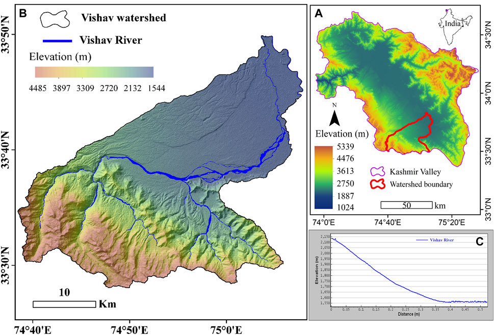
FIGURE 1. (A) Location of the study area in India; (B) Study area (Vishav watershed); (C) Longitudinal river profile of Vishav river.
The watershed endures a varied climate as a result of its terrain with a dramatic decrease in the temperature as we approach the river source at higher altitudes. The watershed is characterized by moderate summers and bitterly cold winters, and it is classed as a temperate alpine climate zone. The watershed mostly receives an average annual precipitation of 1,057 mm from western disturbances, but occasionally also from the southwestern monsoons during a brief period in summer (Zaz et al., 2019). The average yearly snowfall is approximately 670 mm. The mean temperature during the hottest month (July) is 24.6°C and that of the coldest month (January) is 1°C (Zaz and Romshoo, 2013).
Various tectono-geomorphic features, viz, scarp faces, river terraces, triangular facets, knick points, dissected hills, ridges, joints, faults, landslides, etc. are present in the watershed (Wadia, 1931). The watershed is tectonically active and as a result the Vishav River has an asymmetric shape lying more towards the right of the watershed (Figure 1). The gradient of the tributary is very steep with numerous Knick points observed all along its course (Figure 1). Some of the Knick points are very active and have played an important role in the river channel shifting and the consequent erosion of the river banks.
The geology of the watershed comprises of the rocks of Agglomeratic slate, Panjal volcanics, Carbonaceous shale, Triassic Limestone, Hirpur Formation, and recent alluvium which varies from Upper Carboniferous to recent in age (Bhushan et al., 1972). Agglomeratic slates are composed chiefly of quartz. Panjal volcanics of permo-carboniferous age cover the major part of the watershed and comprise augites, andesites, and basalts. Carbonaceous shale comprises fossiliferous shale. Triassic limestones are highly fossiliferous in nature. Hirpur formation comprises unconsolidated sediments of Pleistocene age and preglacial in origin with an estimated thickness of ∼1,700 m. The Recent alluvium is deposited at a place along the rivers and streams.
The datasets used in this study include four DEMs from various sources viz., Advanced Space Borne Thermal Emission and Reflection Radiometer- Global Digital Elevation Model (ASTER-GDEM), Shuttle Radar Topography Mission (SRTM), Advanced Land Observing Satellite (ALOS), and CARTO-DEM for the topographic characterization. The LULC was generated from the Landsat satellite imagery dated 1981/10/24 and 2019/09/08. Moreover, the rainfall data of the nearest stations to the watershed, viz., Qazigund, Kokernag, Pahalgam, and Srinagar stations from 1981 to 2010 was procured from the Indian Meteorological Department for use in this study. The soil texture data were generated from the analysis of the 375 soil samples collected from the watershed. Other data, viz., high-resolution Google Earth images, and ground truth was used for the validation of the LULC. The details of the datasets used in this study are provided in Table 1.
TABLE 1. Datasets used in this study.
The geospatial modeling in a GIS environment is often used for the assessment of various land surface processes due to its ability to integrate inputs from various sources (Moore et al., 1991; Maidment and Djokic, 2000). For the soil erosion estimation, various distributed and empirical models have been developed and applied at various spatial scales like hill slopes, field size, catchment, and basin level (Altaf et al., 2014; Romshoo et al., 2016; Borrelli et al., 2021). Among the globally recognized empirical models for soil erosion estimation, the Universal Soil Loss Equation (USLE), the Modified Universal Soil Loss Equation (MUSLE), and the Revised Universal Soil Loss Equation (RUSLE) have been commonly used the world over (Foster et al., 2003; Hernandez et al., 2012; Saha et al., 2018; Djoukbala et al., 2019). These models are known to predict soil erosion at the watershed scale due to their minimal data requirements and ease of application in the GIS environment. With the additional research, experiments, use of remotely sensed data, and computational advancement which became available over time, the improvement of the USLE led to the development of Revised Universal Soil Loss Equation which includes some new and revised iso-erodent maps, a time-varying approach for soil erodibility factor, a subfactor approach for evaluating the cover-management factor, a new equation to reflect slope length and steepness, and new conservation-practice values (Renard et al., 1997). The model not only provides an estimation of soil loss at the plot scale but also presents the spatial distribution of the soil erosion (Renard et al., 1991). Further, the model is simple, requires fewer data and time to run, and together with the convenience to be used in GIS, the RUSLE is a widely used empirical soil erosion model worldwide (Renard et al., 1991; Bartsch et al., 2002; Dabral et al., 2008; Shinde et al., 2010) and is therefore well suited to be used in the data-scarce mountainous watersheds. The detailed methods regarding the generation of various input parameters, model operation, and accuracy evaluation of the input parameters and validation of the model are briefly discussed in the following sections.
The RUSLE calculates the average annual rate of soil loss (A) in the watershed using the input parameters which are generated, stored, and analyzed in the GIS environment. All the parameters of the RUSLE were converted into raster layers, overlaid, and then multiplied together using the following equation:
where, R = Rainfall erosivity factor; K= Soil erodibility factor; LS = Slope length and slope steepness factor; C = Cover and management factor; and P = Supporting conservation practice factor. The soil loss output was categorized into five erosion classes following the classification system proposed for soil loss (Belayneh et al., 2019). The five soil erosion severity classes are; very slight (0–5 t ha−1 year−1), slight (5–15 t ha−1 year−1), moderate (15–30 t ha−1 year−1), severe (30–50 t ha−1 year−1), and very severe (>50 t ha−1 year−1).
LULC, by affecting the holding capacity of the soils (Sharma et al., 2011), has a profound impact on soil erosion. Land cover with high root biomass will have an impeding impact on the erosion while the human-induced land-use changes exacerbate soil erosion (Gyssels and Poesen, 2003). The Landsat remote sensing data of 1981 and 2019 were used for LULC data generation (Lillesand et al., 1987). Spectral signatures of 13 major LULC classes up to level II were generated using visual image interpretation (Fu, 1976). An extensive field survey was conducted and 311 ground-truth sites for various LULC types were identified and verified with the support of the high-resolution Google Earth satellite images to assess the accuracy of the classified LULC map for the year 2019. The accuracy assessment of various LULC was done using the error matrix. The accuracy assessment provides overall accuracy and overall Kappa (κ). Overall accuracy, the most common error estimate, summarizes the accuracy of a land cover classification, while the Kappa coefficient (K) is the measure of agreement of accuracy. It provides a difference measurement between the observed agreement of two maps and agreement that is contributed by chance alone.
The C-factor accounts for the effect of cropping and management practices on soil erosion (Wischmeier and Smith, 1978) and is derived from LULC which has a direct impact on the rate of erosion (Roose, 1977) and directly impacts several land surface processes including surface hydrology (Romshoo et al., 2011; Badar et al., 2013). The C-factor indicates how the conservation and management plans will affect soil loss. The C-factor reduces the soil loss according to the effectiveness of vegetation and mulch at preventing detachment and transport of soil particles during a rainfall event. Vegetation cover protects soil by dissipating the raindrop energy before it reaches the soil surface. The C-factor values vary between 0 and 1 based on the type of LULC. The C-factor values were calculated from the literature based on the LULC generated for the watershed in this study.
The value of P-factor depends on vegetation type, stage of growth, and cover percentage as soil loss is very sensitive to vegetation cover (Renard et al., 1997). It is the ratio of soil loss from lands with contouring and/or strip cropping to that with straight row farming up-and-down slope. The P-factor varies between 0 and 1 based on the type of land cover with the highest value of 1 assigned to the areas covered by bare soil, built-up areas, and bare rocks where the possibility of erosion rate is very high due to lack of conservation practices. While lower P-factor values were assigned to the rest of the land cover types which represent vegetal cover with some conservation measures in practice. P-factor values were generated from the available literature with the highest value assigned to the areas with no conservation practice and the lowest value of 0.6 was assigned to agriculture in the planar areas of the watershed with moderate slopes and certain conservation practices like contour farming etc. were already in place.
The rainfall erosivity factor (R) is a climate factor used to determine the impact of rain on soil erosion (Wischmeier and Smith, 1978). It has been observed that surface runoff is one of the major reasons for the movement of sediments from the topsoil (Saha et al., 2020). The R-factor is calculated from the long-term summation of annual rainfall energy and maximum 30 min intensity rainfall (Renard et al., 1997; Morgan, 2009). It is one of the important factors in any soil erosion model due to its ability to detach soil particles from one another. Rainfall triggers erosion by the action of runoff and rainfall on the soil surface in MJ mm ha−1 h−1 yr−1. An inverse distance weighting (IDW) interpolation method was used to generate an annual rainfall raster map from four neighboring observation stations around the Vishav watershed. The distribution of the rainfall erosivity factor was calculated using Eq. 2 (Singh et al., 1981). Mean annual precipitation data from 1981 to 2010 was used for the calculation of R-factor by keeping in view the fact that there are no significant changes in precipitation in the region (Murtaza and Romshoo, 2017).
where R is the rainfall erosivity and r is the annual average rainfall in millimeters.
The soil erodibility factor (K) signifies the susceptibility of different soils to erosion (Renard et al., 1997) and is a function of the vulnerability of soil to erosion, the transportability of the sediment, the amount of rainfall, and the rate of runoff. Generally, soils with higher permeability, high levels of organic matter, and improved soil structure have a greater resistance to erosion than the soils having high silt content (Meraj et al., 2018). Erodibility factor map of the study area was generated from the interpolated soil data (Khan S., 2008), based on 375 soil samples collected from the field. The soil erodibility factor (K) was calculated using percent of sand (ms), clay (mc), silt (msilt), organic matter (orgc), soil permeability class, and soil structure class as follows (Williams, 1995):
where,
Topography is an important factor influencing soil erosion. The slope length factor L computes the effect of slope length on erosion and the slope steepness factor S computes the effect of slope steepness on erosion. Values of L and S are relative and represent how erodible a parcel of land with the specific slope length and steepness is relative to the reference plot. The LS factor is computed on the basis of the constant slope exponent (m = 0.5) using the Eq. 8 (Morgan, 2009) and the LS factor estimation was repeated for all the four DEMs.
where LS is slope length and slope steepness factor, Qa is flow accumulation grid, Sg is grid slope (%), M is grid or pixel size (x−y) and y is a dimensionless supporter that assumes the value from 0.2 to 0.5. The value of y varies from 0.2 to 0.5 depending on the slope and slope gradient value, 0.5 is used for the slopes exceeding 4.5%, 0.4 for 3–4.5% slopes, 0.3 for 1–3% slopes, and 0.2 for slopes less than 1%.
The selection of an appropriate DEM for studying land surface processes plays a very important role in minimizing the errors associated with the imprecise topographic characterization extracted from a DEM (De Vente et al., 2009; Coveney and Fotheringham, 2011). In this study, the vertical accuracy of the four-open source DEMs, with the horizontal resolution of ∼30 m viz., ALOS, ASTER, CARTO, and SRTM, was evaluated using the GPS data from 176 ground control points collected from across the watershed (Figure 2). For that purpose, the differences between the elevation values of the DEM and GPS measurements were compared at a pixel level. The GPS measurements were collected using the handheld GPS model- Trimble GCX 6000, mostly from the planar part of the watershed within the elevation range of 1,500–2,200 m. The GPS measurements were projected to the WGS84 horizontal datum in the UTM coordinate system zone 43°N. The point measurements were overlaid upon the four DEMs in order to extract corresponding DEM values for statistical evaluation. The DEM evaluation was done using different statistical measures like mean bias error (Willmott., 1982), root mean square error (Xue et al., 2013), and Nash-Sutcliffe efficiency (Nash and Sutcliffe., 1970). Mean bias error tells us whether the set of measurements consistently underestimate or overestimate the true value and is expressed by the following equation:
where oi is the observed value and pi is the predicted value.
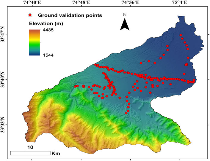
FIGURE 2. Distribution of GPS measurements in the study area used for DEM evaluation.
RMSE indicates how far the observed values differ from the true value (Mukherjee et al., 2012) and is expressed as follows:
where Xobs,i is the observation value and Xmodel,i is the forecast value.
Nash-Sutcliffe efficiency (NSE) was used to determine the match between the GCPs and the DEM values. The NSE value = 1 corresponds to a perfect match between the observed and assumed value (McCuen et al., 2006). NSE is expressed as follows:
where OBSi is the observation value and SIMi is the forecast value and
Apart from the above statistical evaluation, a visual assessment of the erosion pattern and distribution derived from the DEMs was done by comparison with the erosion features and patterns present on the high-resolution satellite data.
Validation of the soil erosion estimated from the RUSLE model is important to ascertain the accuracy of the model output. However, due to the lack of soil erosion observations in the Himalayas, we are constrained to quantitatively assess the accuracy of the soil erosion estimates from the RUSLE model. Therefore, the model output was evaluated and correlated with the land degradation indicators prepared at 1:30 k scale and generated using three-season Landsat-8 OLI data for the year-2017–18 (ISRO, 2016; 2018). The land degradation map showing vegetal degradation, water erosion, and waterlogging at three different severity levels, was correlated with the modeled soil erosion maps.
The spatial distribution of LULC observed in the study area during 1981 and 2019 is shown in Figures 3A,A′ and the data is provided in Table 2. Analysis of the data shows that there are significant changes in LULC over the study area during the last 38 years. The maximum LULC change is observed in agriculture which has reduced from 38% in 1981 to 9.1% in 2019. Correspondingly, the horticulture lands show an increasing trend from 7.6% in 1981 to 26.6% in 2019. Forest land has decreased from 22.7% in 1981 to 13.7% in 2019 which has led to the expansion of degraded forests from just 0.9–10.8% during the same period. The built-up area in the watershed has increased from 0.4 to 3.9% during the period. Barren land (0.3%) shows no significant change between the two dates. Plantation shows an increasing trend from 2.7% in 1981 to 9% in 2019. The river bed shows a slight increase from 2.3 to 2.4% during the period. The watercourses have shrunk from 0.9% in 1981 to 0.4% in 2019. However, the changes in the water could be due to the fluctuations in the water levels between 1981 and 2019 as the streamflow has significantly depleted in the Jhelum over time (Romshoo et al., 2015). Scrublands show a slight increase from 12.8% in 1981 to 13.7% in 2019. Pasturelands decreased in extent from 2% in 1981 to 1.1% in 2019. For the accuracy assessment of the LULC of the year 2019 using 311 sample points, the overall accuracy of the LULC delineated from 2019 satellite data is 91% and the Kappa coefficient is 0.85.
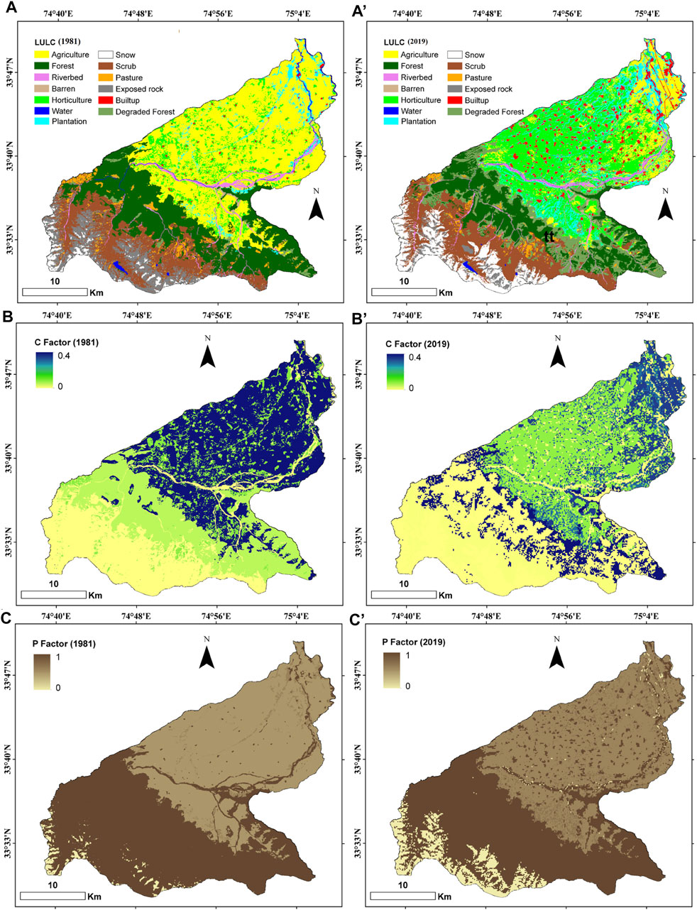
FIGURE 3. LULC map of the study area during (A) 1981 and (A′) 2019; Crop management factor (C) map during (B) 1981 and (B′) 2019; Conservation practices factor (P) map during (C) 1981 and (C′) 2019.
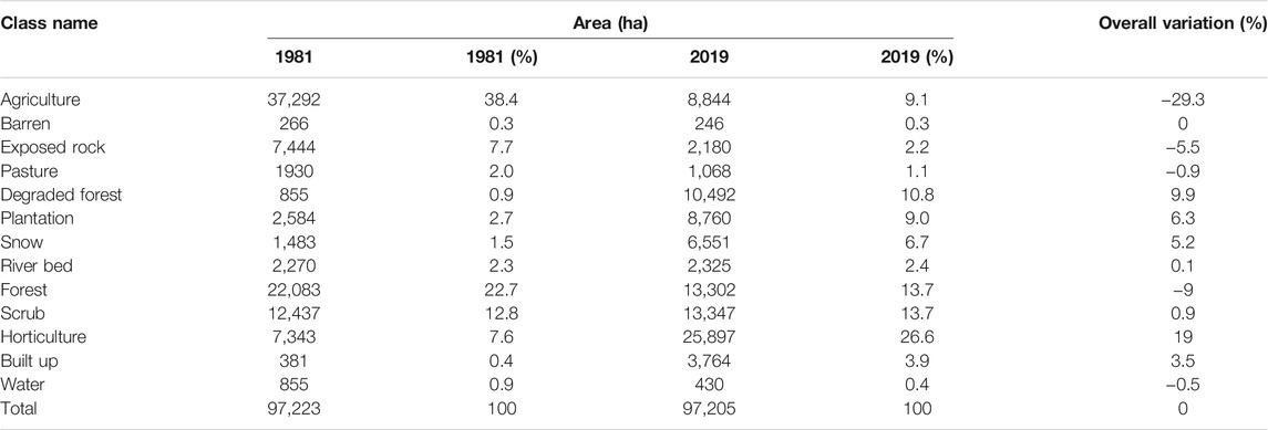
TABLE 2. LULC change observed from 1981 to 2019 in the study area.
Crop management factor represents the relative effectiveness of soil and crop management systems in preventing soil loss (Roose, 1977) and is considered as the most important factor in management programs in erosion vulnerable areas for proper land practices (Teh, 2011; Saha et al., 2021). Figures 3B,B′ shows the C factor distribution derived from the LULC map of the study area in 1981 and 2019. The C-factor values spatiotemporally varied due to the variability of the LULC in the watershed, such as the higher C factor values were often widespread along the valley plains in 1981, and then declined due to the decreased agricultural activities in the year 2019. Nevertheless, the values in the mountainous areas, tended to decrease, resulting from the presence of forests and semi-natural areas like pasturelands. In the case of the degraded forests and scrublands, the increased soil erosion risk was observed, primarily, because the P-factor values for these LULC classes have typically shown a decreasing trend over the years due to their Spatio-temporal variability. The resulting maps illustrate an increasing trend in artificial surfaces and horticulture and a decreasing trend in agricultural areas and forests.
The factor represents the effect of practices that reduce the runoff rate and check the soil loss (Stone and Hilborn, 2000). Figures 3C,C′ shows the P-factor distribution estimated from the LULC maps of 1981 and 2019. P-factor values vary from 0 to 1 where the highest value is allocated to LULC zone with no management practices (scrub and barren land) and the lowest values are assigned to LULC type like built-up-land and agriculture with contour cropping. More effective the conservation and management practices, the lower the p-value.
The spatial distribution of the rainfall erosivity factor (R) is provided in Figure 4A. It was observed that the values of R in the Vishav watershed range from 457 to 512 MJ mm/ha-h-yr. Around 300 km2 (30%) of the Vishav watershed has R ranging from 495 to 512 MJ mm/ha-h-yr, 407 km2 (41%) is covered by the range 477–494 MJ mm/ha-h-yr and 289 km2 (29%) has R ranging from 457 to 476 MJ mm/ha-h-yr. Since the R-factor is a function of the amount of rainfall, therefore, the more the rainfall the more soil will get detached from the land (Wischmeier and Smith, 1978).
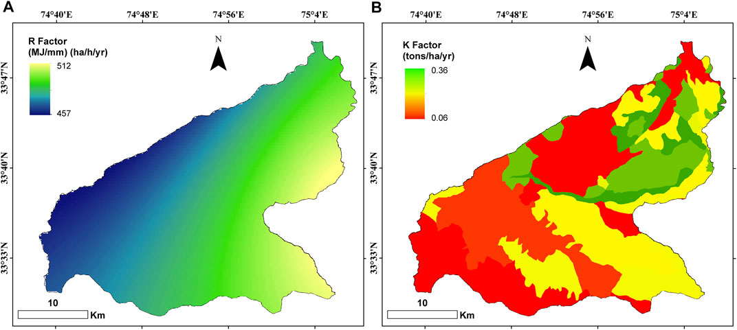
FIGURE 4. (A) Rainfall erosivity factor (R) map of the study area; (B) Soil erodibility factor (K) map of the study area.
The distribution of the soil erodibility factor (K) is provided in Figure 4B. It is observed that around 37% of the watershed is covered by sandy soils which are prone to erosion. K-factor varied from 0.063 to 0.361 T ha−1 yr−1. The values of K-factor decreased from plains to the higher altitudes due to the presence of rocky outcrops and seasonal snow cover at high altitudes. K-factor was found to be lower in the cultivated areas due to the application of chemical fertilizers and single-crop cultivation activity (Ayoubi et al., 2012).
The slope of the study area ranges from 0 to 72.8° (324.3%) with the steepest slopes located in the south-western part of the watershed which is usually susceptible to soil erosion compared to the flatter areas on the northern side. LS factor values were also higher along the flow path, with a rapid increase at zones of flow concentration. The LS value was estimated by using a multiple flow direction approach which showed significant variability among different DEMs used in this study. The higher values of the LS factor characterize steep slopes (Moore and Wilson, 1992; Prasannakumar et al., 2012) which were found on the higher south-western reaches of the watershed facing severe erosion problems. The CARTO, SRTM, and ALOS DEMs possess comparably similar LS factor values as shown in Table 3. It is pertinent to mention that all other parameters of the RUSLE equation were kept constant while the LS factor varied with the changing DEM to determine the impact on DEM quality on soil erosion.
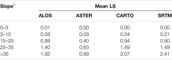
TABLE 3. Mean LS-factor values for different slope categories derived from different DEMs in the study area.
The DEMs were compared with the 176 GPS measurements in terms of the elevation and the absolute differences in elevation were calculated and evaluated using various statistical measures (Table 4). The Root Mean Square Error (RMSE) of CARTO, ASTER, SRTM, and ALOS DEMs was 18.2, 35, 35.7, and 36.9 m with the mean bias of −9.11, 33.65, 32.33, and 30.88 m, respectively. The CARTO DEM showed a negative bias which suggests underestimation of the elevation values but the other three DEMs showed a positive bias, i.e., overestimation of the elevation values. The RMSE for ALOS, SRTM, and ASTER observed in this study is higher compared to that reported in other studies (Team, 2009; Jarvis et al., 2012; Takaku et al., 2014). In the case of the NSE, the GPS measurements showed the best agreement with the elevation values in case of the CARTO DEM followed by the ASTER, SRTM, and ALOS DEMs yielding NSE values of 0.99, 0.96, 0.95, and 0.95, respectively.
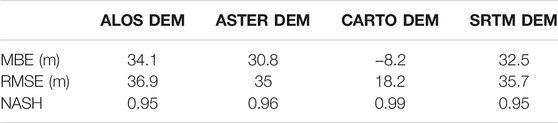
TABLE 4. Statistical evaluation of different DEMs on basis of comparison with the GPS measurements over the study area using ground control points.
The soil erosion estimates based on the use of four DEMs vary significantly due to the varying topographic characterization provided by the DEMs, mainly a variation of slope gradient and therefore the variation in the LS factor. It was observed that the erosion estimate derived from the CARTO, SRTM, and ALOS DEMs have a similar spatial pattern while the soil erosion estimates derived from the ASTER DEM show a comparatively slightly different pattern. This variation in the amount and distribution of erosion from the four DEMs is due to the inherent errors associated with the DEMs observed both in the planar and undulating areas of the watershed. As evident from Figure 5, the soil erosion is observed to be higher along the higher regions of the Pir Panjal range in the southern and south-eastern part of the watershed, having steep slopes as compared to the planar areas of the watershed. The erosion estimates generated from the SRTM DEM and the ALOS DEM show a good correlation with each other in the plain areas of the watershed. The erosion estimates from the CARTO DEM show a close correlation to those derived from the SRTM and ALOS DEMs in the higher reaches of the watershed. Among the four erosion prediction estimates, the erosion from the 30-m ASTER underestimates the erosion rate by ∼90% over the flat and moderate slope terrains due to lower observed mean LS values. The mean annual soil loss estimates derived from the watershed using ALOS and SRTM DEMs are approximately 2.8 tons/ha/yr. The CARTO and ASTER DEM estimates are around 2.9 tons/ha/yr and 1.2 tons/ha/yr respectively (Figure 5). The total estimated soil loss from the watershed based on the use of the four DEMs is shown in Table 5 which indicates a significant variation of the soil erosion estimates attributed to the differences in the topographic characterization of the watershed extracted from the four DEMs. It was observed that the soil erosion estimates from the ASTER DEM significantly vary (underestimation) from the estimates obtained from the other three DEMs. This demonstrates the importance of and need for making the right choice of the DEM for accurate assessment of the soil erosion at the watershed scale.
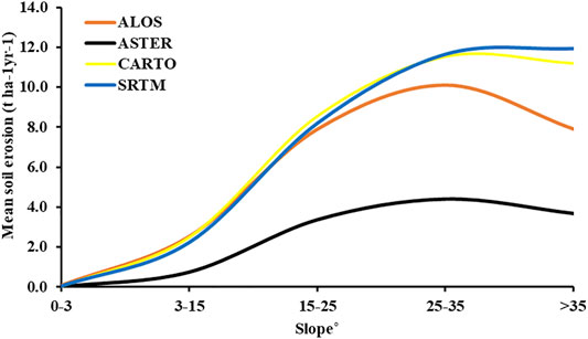
FIGURE 5. Comparison of the mean soil erosion rates under various slope categories using the four DEMs used in this study.
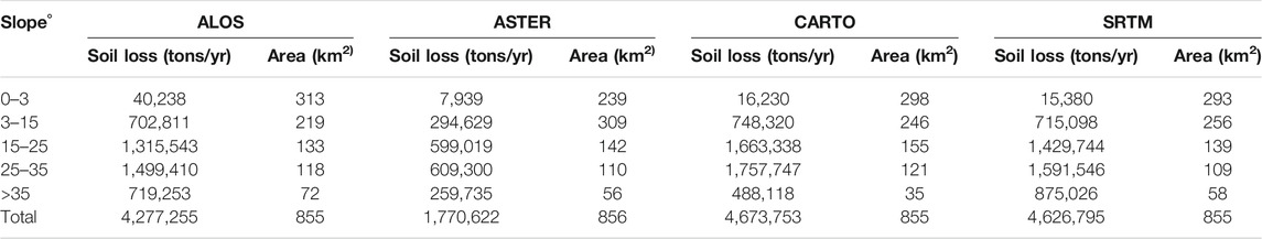
TABLE 5. Area under different slope categories provided by the four DEMs and the total soil loss thereof.
The LULC plays a significant role in controlling soil erosion by reducing the direct impacts of raindrops on the soil, enhancing the organic matter content, increasing the infiltration rate of water, reducing the velocity of runoff, and reducing the transportation of sediments on the soil surface (ICIMOD, 1994). Therefore, any change in the LULC, whether driven by natural or anthropogenic activities, would significantly affect the rate of soil erosion (Borrelli et al., 2013). The LULC of 1981 and 2019 along with the other parameters related to climate, soils, and topography was used to determine the impact of LULC on soil erosion. The soil loss estimates from the watershed for 1981 and 2019 are shown in Table 6. As can be seen from the analysis of the data provided in the table, there is an overall increase in the mean soil erosion from the watershed due to the LULC change observed between 1981 and 2019. The soil erosion has increased by almost double from 23.93 t ha−1 year−1 in 1981 to 46.24 t ha−1 year−1 in 2019. A decrease in erosion is observed in some LULC classes from 1981 to 2019 due to the shrinkage in the LULC type. For example, the erosion from the agricultural lands in the watershed decreased by 18.6% during the period due to the conversion of them and of paddy lands to other land classes. Similarly, the pasturelands show lower erosion indicating a decrease of 3.9% (Table 6). Contrarily, the soil erosion under the degraded forests, scrublands, and horticulture is showing a significant increase due to the increase in the area under these LULC classes in 2019. The maximum soil erosion is observed from the degraded forest which has increased from 6% in 1981 to 57% in 2019. The degraded forest LULC type is mostly situated on denudated and steep slopes with little tree cover directly exposed to the raindrop impact which accelerates the detachment, removal, and transportation of soil particles. The LULC based soil loss estimates from the watershed for the two periods is presented in Figures 6A,B, 7A,B and Table 6 which provides information about the soil erosion changes as a function of the land system changes in the watershed observed from 1981 to 2019.
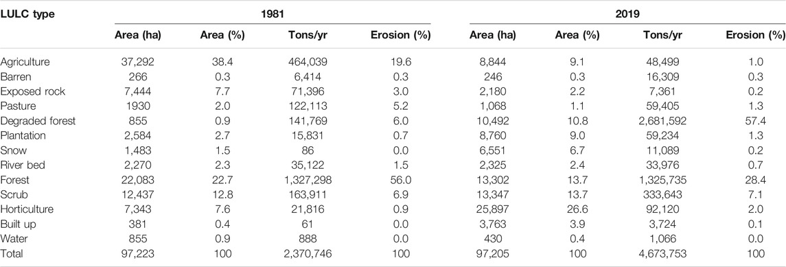
TABLE 6. Soil erosion estimated under each LULC type in the study area during 1981 and 2019 using CARTO DEM.
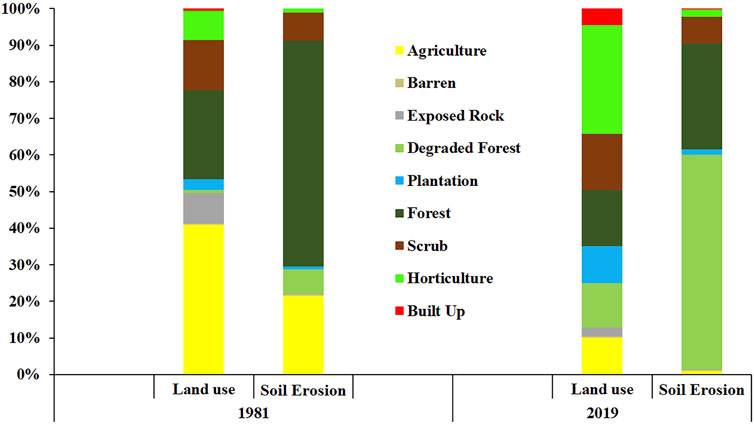
FIGURE 6. Soil erosion under different LULC classes during 1981 and 2019.
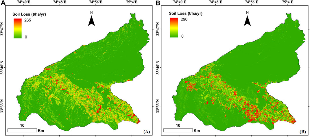
FIGURE 7. Spatial distribution of soil erosion in the study area during (A) 1981 and (B) 2019 using CARTO DEM.
The estimated soil erosion from the study area was classified into five severity classes. The results for the year 1981 showed that ∼85% (829 km2) of the study area is under very slight soil erosion, followed by 12% (118 km2) of the watershed area falling under the slight soil erosion class and only 2% (20 km2) under moderate erosion class. The watershed area categorized under severe to very severe erosion was a meager 0.37% (4 km2) and 0.33% (3 km2) as given in Table 7. In the year 2019, 84% (820 km2) of the area comes under the very slight erosion class followed by 8% (82 km2) under slight erosion risk. While 3.07% (30 km2) of the watershed is facing moderate soil erosion. Watershed areas under severe and very severe soil erosion classes in 2019 increased by 1.5 and 1.9%, respectively due to LULC changes observed during the period which showed an increase in the area under these two erosion classes from 14 km2 in 1981 to 19 km2 in 2019. The two classes are characterized by steep slopes with little or no vegetal cover. There is an increase in the area under the moderate, severe, and very severe soil erosion classes in 2019 due to the increase in the area under horticulture and degraded forest observed from the LULC data during 1981–2019. Similarly, the watershed area under severe and very severe soil erosion classes has increased from 0.37 to 1.82% and 0.33–2.23% respectively from 1981 to 2019 which implies a loss of the forests and other land degradation processes in the watershed.
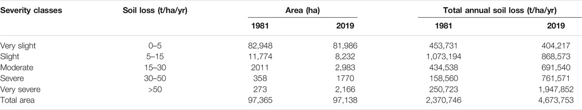
TABLE 7. Total annual soil loss under various soil erosion severity classes during 1981 and 2019 using CARTO DEM.
In absence of the observed soil erosion data in the watershed, the validation of the simulated soil erosion estimates obtained in this study was done using the land degradation maps generated for the study area. The simulated soil erosion estimates showed an overall good correlation with the land degradation map generated at 1:30 k scale for the watershed (Figure 8). The watershed areas under low and very low soil erosion class (0–2 t ha−1 yr−1) correlate well with the lowest level of the land degradation severity classes, like {Fv1(Forest, vegetal degradation, low severity), Sv1(Land with scrub, vegetal degradation, low severity), Dw1(unirrigated-agriculture, water erosion, low severity)} or no apparent land degradation class (NAD). The watershed areas where the rate of simulated soil erosion is >5 t ha−1 yr−1 but <10 t ha−1 yr−1 correspond well with the moderate or severe degradation severity classes like {Fw2 (Forest, water erosion, moderate severity), Fv2 (Forest, vegetal degradation, moderate severity); Sv2 (Land with scrub, vegetal degradation, moderate severity)}. The watershed areas that showed the highest rate of soil erosion i.e., >10 t ha−1 yr−1 showed high correspondence with the land degradation indicator map classes having the high severity, like {Fw3 (Forest, water erosion, moderate severity), Fv3 (Forest, vegetal degradation, severe severity) and Sv3 (Land with scrub, vegetal degradation, severe severity)}.
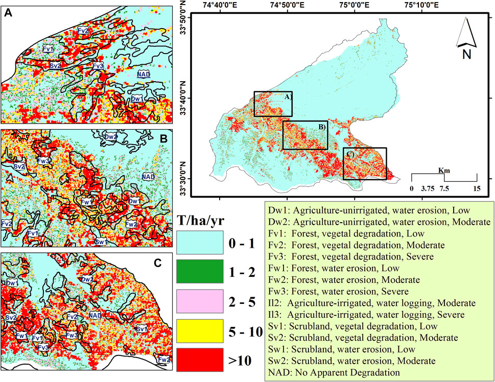
FIGURE 8. Validation of the estimated soil erosion for the year 2019 generated using the land degradation map.
The Revised Universal Soil Loss Equation (RUSLE) was used in this study to quantify soil erosion from the data-scarce Vishav watershed in the Kashmir Himalaya. Since the topography is a major contributor to the transport of the soil from a watershed, it was therefore thought necessary to choose the best of the publicly available digital topographic datasets for accurate topographic characterization of the watershed so that the errors associated with soil erosion estimates due to the imprecise representation of the topography are minimized. The evaluation of the DEMs with respect to the GPS observations using various statistical tests showed that the CARTO DEM has better accuracy among the four evaluated topographic datasets. The soil erosion estimates using CARTO DEM and 2019 LULC showed good validation with the land degradation indicator maps. The study also revealed that the LULC changes observed in the watershed from 1981 to 2019, mainly driven by anthropogenic factors, have led to the doubling of the soil erosion from 23.93 t ha−1 year−1 in 1981 to 46.24 t ha−1 year−1 in 2019. Degradation of forests and the expansion of cultivation on the degraded lands on steep-slope in the mountainous areas of the watershed and other land system changes observed during the past 28 years together with the anthropogenic pressures and the consequent land degradation processes are the root cause of the observed soil erosion from the watershed. Use of the precise set of topographic characteristics from the most reliable publicly available DEM remotely sensed and extensively validated LULC, and lab-observed soil properties in the GIS framework facilitated the quantification of soil erosion estimates at the watershed scale. However, the inadequate representation of the precipitation record in the watershed affects the precise quantification of two important factors; rainfall erosivity and soil erodibility, and thus adding uncertainty to the soil erosion estimates simulated in this study.
Choosing the most appropriate publicly available DEMs provided in this study would help researchers in the selection of the precise topographic characteristics to model various land surface processes at watershed scale in the data-scarce mountainous terrains where the topography is the dominant factor controlling various processes. However, the DEMs need to be validated with a larger set of ground control points from a wide range of topography and the study needs to be replicated in different topographic settings to draw more valid and universal conclusions about the suitability of the publicly available DEMs for characterizing land surface processes.
It is further believed that the findings from this research shall inform the policymaking on land use planning, soil and water conservation, and environmental degradation so that the appropriate strategies are devised for the sustainable development of land and water resources in the ecologically fragile Kashmir Himalaya and other mountainous regions in the Indian Himalaya and beyond.
The original contributions presented in the study are included in the article/Supplementary Material, further inquiries can be directed to the corresponding author.
SAR conceptualized the idea, supervised the research and wrote the manuscript with contributions from AY and SA. SAR, AY and SA together analysed the data and results. AY generated the inputs, ran simulations in GIS and created figures and tables. AY and SA conducted the field validation of the LULC data and DEMs. MA conducted the validation of the soil erosion output.
The research work was conducted as part of the Ministry of Environment, Forests and Climate Change (MoEF&CC), Government of India, New Delhi sponsored research project under National Mission on Himalayan Studies (NMHS) titled “Enhancement of the quality of livelihood opportunities and resilience for the people in the Indian Himalayas…”
The authors declare that the research was conducted in the absence of any commercial or financial relationships that could be construed as a potential conflict of interest.
All claims expressed in this article are solely those of the authors and do not necessarily represent those of their affiliated organizations, or those of the publisher, the editors and the reviewers. Any product that may be evaluated in this article, or claim that may be made by its manufacturer, is not guaranteed or endorsed by the publisher.
The financial assistance received under the project to accomplish this research is thankfully acknowledged. The authors express their gratitude to the two reviewers for their valuable comments and suggestions that improved the quality of the manuscript.
Altaf, S., Meraj, G., and Romshoo, S. A. (2014). Morphometry and Land Cover Based Multi-Criteria Analysis for Assessing the Soil Erosion Susceptibility of the Western Himalayan Watershed. Environ. Monit. Assess. 186, 8391–8412. doi:10.1007/s10661-014-4012-2
Amin, M., and Romshoo, S. A. (2019). Comparative Assessment of Soil Erosion Modelling Approaches in a Himalayan Watershed. Model. Earth Syst. Environ. 5 (1), 175–192. doi:10.1007/s40808-018-0526-x
Arabameri, A., Rezaie, F., Pal, S. C., Cerda, A., Saha, A., Chakrabortty, R., et al. (2021). Modelling of Piping Collapses and Gully Headcut Landforms: Evaluating Topographic Variables from Different Types of DEM. Geosci. Front. 12, 101230. doi:10.1016/j.gsf.2021.101230
Ayoubi, S., Mokhtari Karchegani, P., Mosaddeghi, M. R., and Honarjoo, N. (2012). Soil Aggregation and Organic Carbon as Affected by Topography and Land Use Change in Western Iran. Soil Tillage Res. 121, 18–26. doi:10.1016/j.still.2012.01.011
Badar, B., Romshoo, S. A., and Khan, M. A. (2013). Integrating Biophysical and Socioeconomic Information for Prioritizing Watersheds in a Kashmir Himalayan lake: A Remote Sensing and GIS Approach. Environ. Monit. Assess. 185, 6419–6445. doi:10.1007/s10661-012-3035-9
Barrow, C. J. (1991). Land Degradation: Development and Breakdown of Terrestrial Environments. Cambridge,U K: Cambridge University Press.
Bartsch, K. P., Van Miegroet, H., Boettinger, J., and Dobrowolski, J. P. (2002). Using Empirical Erosion Models and GIS to Determine Erosion Risk at Camp Williams, Utah. J. Soil Water Conserv 57 (1), 29–37.
Belayneh, M., Yirgu, T., and Tsegaye, D. (2019). Potential Soil Erosion Estimation and Area Prioritization for Better Conservation Planning in Gumara Watershed Using RUSLE and GIS Techniques. Environ. Syst. Res. 8 (1), 1–17. doi:10.1186/s40068-019-0149-x
Bhushan, B., Raina, K. B., Maiti, R. P., and Pathak, S. C. (1972). Geological Mapping of the Part of the Pir Panjal Range in Kulgam Tehsil, Anantnag District, Jammu and Kashmir State, India. Northern Region, Lucknow: Geological Survey of India, 1–9.
Boggs, G., Devonport, C., Evans, K., and Puig, P. (2001). GIS-based Rapid Assessment of Erosion Risk in a Small Catchment in the Wet/dry Tropics of Australia. Land Degrad. Dev. 12 (5), 417–434. doi:10.1002/ldr.457
Borrelli, P., Alewell, C., Alvarez, P., Anache, J. A. A., Baartman, J., Ballabio, C., et al. (2021). Soil Erosion Modelling: A Global Review and Statistical Analysis. Sci. Total Environ. 780, 146494. doi:10.1016/j.scitotenv.2021.146494
Borrelli, P., Hoelzmann, P., Knitter, D., and Schütt, B. (2013). Late Quaternary Soil Erosion and Landscape Development in the Apennine Region (central Italy). Quat. Int. 312, 96–108. doi:10.1016/j.quaint.2012.12.007
Cerri, C. E. P., Demattě, J. A. M., Ballester, M. V. R., Martinelli, L. A., Victoria, R. L., and Roose, E. (2001). GIS Erosion Risk Assessment of the Piracicaba River Basin, Southeastern Brazil. Mapp. Sci. Remote Sensing 38, 157–171. doi:10.1080/07493878.2001.10642173
Chang, K.-t., and Tsai, B.-w. (1991). The Effect of DEM Resolution on Slope and Aspect Mapping. Cartography Geogr. Inf. Syst. 18 (1), 69–77. doi:10.1559/152304091783805626
Chowdhuri, I., Pal, S. C., Saha, A., Chakrabortty, R., and Roy, P. (2021). Evaluation of Different DEMs for Gully Erosion Susceptibility Mapping Using In-Situ Field Measurement and Validation. Ecol. Inform. 65, 101425. doi:10.1016/j.ecoinf.2021.101425
Coveney, S., and Fotheringham, A. S. (2011). The Impact of DEM Data Source on Prediction of Flooding and Erosion Risk Due to Sea-Level Rise. Int. J. Geographical Inf. Sci. 25 (7), 1191–1211. doi:10.1080/13658816.2010.545064
Dabral, P. P., Baithuri, N., and Pandey, A. (2008). Soil Erosion Assessment in a Hilly Catchment of North Eastern India Using USLE, GIS and Remote Sensing. Water Resour. Manage. 22 (12), 1783–1798. doi:10.1007/s11269-008-9253-9
Dar, R. A., Romshoo, S. A., Chandra, R., and Ahmad, I. (2014). Tectono-geomorphic Study of the Karewa Basin of Kashmir Valley. J. Asian Earth Sci. 92, 143–156. doi:10.1016/j.jseaes.2014.06.018
De Vente, J., Poesen, J., Govers, G., and Boix-Fayos, C. (2009). The Implications of Data Selection for Regional Erosion and Sediment Yield Modelling. Earth Surf. Process. Landforms 34 (15), 1994–2007. doi:10.1002/esp.1884
Djoukbala, O., Hasbaia, M., Benselama, O., and Mazour, M. (2019). Comparison of the Erosion Prediction Models from USLE, MUSLE and RUSLE in a Mediterranean Watershed, Case of Wadi Gazouana (N-W of Algeria). Model. Earth Syst. Environ. 5 (2), 725–743. doi:10.1007/s40808-018-0562-6
D. R. Maidment, and D. Djokic (Editors) (2000). Hydrologic and Hydraulic Modeling Support: With Geographic Information Systems (West Redlands, California, United States: ESRI, Inc).
Florinsky, I. V. (1998). Accuracy of Local Topographic Variables Derived from Digital Elevation Models. Int. J. Geographical Inf. Sci. 12, 47–62. doi:10.1080/136588198242003
Foster, G. R., Toy, T. E., and Renard, K. G. (2003). Comparison of the USLE, RUSLE1. 06c, and RUSLE2 for Application to Highly Disturbed lands. In First Interagency Conference on Research in Watersheds. 27(30), 154–160.
Gyssels, G., and Poesen, J. (2003). The Importance of Plant Root Characteristics in Controlling Concentrated Flow Erosion Rates. Earth Surf. Process. Landforms 28 (4), 371–384. doi:10.1002/esp.447
Hernandez, E. C., Henderson, A., and Oliver, D. P. (2012). Effects of changing land use in the Pagsanjan-Lumban catchment on suspended sediment loads to Laguna de Bay, Philippines. Agric. Water Management 106, 8–16. doi:10.1016/j.agwat.2011.08.012
ICIMOD (1994). “Mountain Environment and Development: Constraints and Opportunities,” in Proceedings of the and Papers of the ICIMOD 10th Anniversary Symposium held on 1-2 Dec 1993, Kathmandu, Nepal, 1-2 Dec 1993.
ISRO (2016). Desertification and Land Degradation Atlas of India (Based on IRS AWiFS Data of 2011-13 and 2003-05). ISRO, Ahmedabad, India: Ahmedabad: Space Applications Centre, 219.
ISRO (2018). Desertification and Land Degradation, Atlas of Selected Districts of India (Based on IRS LISS III Data of 2011-13 and 2003-05) Volume -1. ISRO, Ahmedabad, India: Ahmedabad: Space Applications Centre, 148.
Jain, S. K., Kumar, S., and Varghese, J. (2001). Estimation of Soil Erosion for a Himalayan Watershed Using GIS Technique. Water Resour. Manag. 15 (1), 41–54. doi:10.1023/a:1012246029263
Jarvis, A., Reuter, H. I., Nelson, A., and Guevara, E. (2008). Hole-filled SRTM for the globe Version 4. Available from the CGIAR-CSI SRTM 90m Database. Cali, Colombia: CGIAR Consortium for Spatial Information. Available at: http://srtm.csi.cgiar.org.
Jenson, S. K. (1991). Applications of Hydrologic Information Automatically Extracted from Digital Elevation Models. Hydrol. Process. 5 (1), 31–44. doi:10.1002/hyp.3360050104
Kalambukattu, J., and Kumar, S. (2017). Modelling Soil Erosion Risk in a Mountainous Watershed of Mid-himalaya by Integrating RUSLE Model with GIS. Eurasian J. Soil Sci. 6 (2), 92. doi:10.18393/ejss.286442
Khan, S., and Romshoo, S. A. (2008). Integrated Analysis of Geomorphic, Pedologic and Remote Sensing Data for Digital Soil Mapping. J. Himalayan Ecol. Sustain. Dev. 3, 84–93. doi:10.36106/gjra
Kienzle, S. (2004). The Effect of DEM Raster Resolution on First Order, Second Order and Compound Terrain Derivatives. Trans. GIS 8, 83–111. doi:10.1111/j.1467-9671.2004.00169.x
Kolli, M. K., Opp, C., and Groll, M. (2021). Estimation of Soil Erosion and Sediment Yield Concentration across the Kolleru Lake Catchment Using GIS. Environ. Earth Sci. 80 (4), 1–14. doi:10.1007/s12665-021-09443-7
Lal, R. (1998). Soil Erosion Impact on Agronomic Productivity and Environment Quality. Crit. Rev. Plant Sci. 17 (4), 319–464. doi:10.1080/07352689891304249
Lillesand, T. M., and KieferChipman, R. W. J. W. (1987). Remote Sensing and Image Interpretation. New York: John Wiley & Sons.
Mahapatra, S. K., Walia, C. S., Sidhu, G. S., Rana, K. P. C., and Lal, T. (2000). Characterization and Classification of the Soils of Different Physiographic Units in the Subhumid Eco-System of Kashmir Region. J. Indian Soc. Soil Sci 48 (3), 572–577.
McCuen, R. H., Knight, Z., and Cutter, A. G. (2006). Evaluation of the Nash-Sutcliffe Efficiency Index. J. Hydrol. Eng. 11 (6), 597–602. doi:10.1061/(asce)1084-0699(2006)11:6(597)
Meraj, G., Romshoo, S. A., Ayoub, S., and Altaf, S. (2018). Geoinformatics Based Approach for Estimating the Sediment Yield of the Mountainous Watersheds in Kashmir Himalaya, India. Geocarto Int. 33 (10), 1114–1138. doi:10.1080/10106049.2017.1333536
Moore, I. D., and Wilson, J. P. (1992). Length-slope Factors for the Revised Universal Soil Loss Equation: Simplified Method of Estimation. J. Soil Water Conserv 47 (5), 423–428.
Moore, I. D., Grayson, R. B., and Ladson, A. R. (1991). Digital Terrain Modelling: A Review of Hydrological, Geomorphological, and Biological Applications. Hydrol. Process. 5, 3–30. doi:10.1002/hyp.3360050103
Morgan, R. P. C., and Nearing, M. A. (2002). “Soil Erosion Models: Present and Future. In Man and Soil at the Third Millennium,” in Proceedings International Congress of the European Society for Soil Conservation, Valencia, Spain, 28 March-1 April, 2000, 187–205.
Morgan, R. P. C. (2009). Soil Erosion and Conservation. Hoboken, New Jersey, United States: John Wiley & Sons.
Mukherjee, S., Joshi, P. K., Mukherjee, S., Ghosh, A., Garg, R. D., and Mukhopadhyay, A. (2012). Evaluation of Vertical Accuracy of Open Source Digital Elevation Model (DEM). Int. J. Appl. Earth Obs Geoinf 21, 205–217. doi:10.1016/j.jag.2012.09.004
Murtaza, K. O., and Romshoo, S. A. (2017). Recent Glacier Changes in the Kashmir alpine Himalayas, India. Geocarto Int. 32 (2), 188–205. doi:10.1080/10106049.2015.1132482
Narayana, D. V. V., and Babu, R. (1983). Estimation of Soil Erosion in India. J. Irrigation Drainage Eng. 109 (4), 419–434. doi:10.1061/(asce)0733-9437(1983)109:4(419)
Nash, J. E., and Sutcliffe, J. V. (1970). River Flow Forecasting through Conceptual Models Part I - A Discussion of Principles. J. Hydrol. 10 (3), 282–290. doi:10.1016/0022-1694(70)90255-6
Pal, S. C., Chakrabortty, R., Arabameri, A., Santosh, M., Saha, A., Chowdhuri, I., et al. (2021). Chemical Weathering and Gully Erosion Causing Land Degradation in a Complex River basin of Eastern India: an Integrated Field, Analytical and Artificial Intelligence Approach. Nat. Hazards, 1–33. doi:10.1007/s11069-021-04971-8
Pal, S. C., Chakrabortty, R., Roy, P., Chowdhuri, I., Das, B., Saha, A., et al. (2021). Changing Climate and Land Use of 21st century Influences Soil Erosion in India. Gondwana Res. 94, 164–185. doi:10.1016/j.gr.2021.02.021
Prasannakumar, V., Vijith, H., Abinod, S., and Geetha, N. (2012). Estimation of Soil Erosion Risk within a Small Mountainous Sub-watershed in Kerala, India, Using Revised Universal Soil Loss Equation (RUSLE) and Geo-Information Technology. Geosci. Front. 3, 209–215. doi:10.1016/j.gsf.2011.11.003
Raza, M., Ahmad, A., and Mohammad, A. (1978). The Valley of Kashmir: A Geographical Interpretation, Vol, 1: The Land. New Delhi: Vikas Publishing House Pvt., Ltd., 1–59.
Renard, K. G., Foster, G. R., Weesies, G. A., and Porter, J. P. (1991). RUSLE: Revised Universal Soil Loss Equation. J. Soil Water Conserv. 46 (1), 30–33.
Renard, K. G. (1997). Predicting Soil Erosion by Water: A Guide to Conservation Planning with the Revised Universal Soil Loss Equation (RUSLE). Washington, DC: United States Government Printing.
Romshoo, S. A., Altaf, S., Rashid, I., and Dar, R. A. (2017). Climatic, Geomorphic and Anthropogenic Drivers of the 2014 Extreme Flooding in the Jhelum basin of Kashmir, India. Geomatics, Nat. Hazards Risk 9 (1), 224–248. doi:10.1080/19475705.2017.1417332
Romshoo, S. A., Ali, N., and Rashid, I. (2011). Geoinformatics for Characterizing and Understanding the Spatio-Temporal Dynamics (1969 to 2008) of Hokersar Wetland in Kashmir Himalayas. Int. J. Phys. Sci. 6 (5), 1026–1038.
Romshoo, S. A., Amin, M., and Sastry, I. K. L. N. (2016). Soil Erosion Estimation of Lidder Watershed, Kashmir Himalaya Using Morgan-Morgan-Finney Model in GIS Environment. J. Himalayan Ecol. Sustain. Dev. 11, 3–20.
Romshoo, S. A., Amin, M., Sastry, K. L. N., and Parmar, M. (2020). Integration of Social, Economic and Environmental Factors in GIS for Land Degradation Vulnerability Assessment in the Pir Panjal Himalaya, Kashmir, India. Appl. Geogr. 125, 102307. doi:10.1016/j.apgeog.2020.102307
Romshoo, S. A., Dar, R. A., Rashid, I., Marazi, A., Ali, N., and Zaz, S. N. (2015). Implications of Shrinking Cryosphere under Changing Climate on the Streamflows in the Lidder Catchment in the Upper Indus basin, India. Arctic, Antarctic, Alpine Res. 47, 627–644. doi:10.1657/aaar0014-088
Roose, E. J. (1977). “Use of the Universal Soil Loss Equation to Predict Erosion in West Africa,” in Soil Erosion: Prediction and Control (Ankeny, Iowa: Soil Conservation Society of America Ankeny), 21, 60–74.
Saha, A., Ghosh, M., and Pal, S. C. (2020). “Understanding the Morphology and Development of a Rill-Gully: an Empirical Study of Khoai Badland, West Bengal, India,” in Gully Erosion Studies from India and Surrounding Regions (Cham: Springer), 147–161. doi:10.1007/978-3-030-23243-6_9
Saha, A., Ghosh, P., and Mitra, B. (2018). GIS Based Soil Erosion Estimation Using RUSLE Model: a Case Study of Upper Kangsabati Watershed, West Bengal, India. Int. J. Environ. Sci. Nat. Resour. 13 (5), 119–126. doi:10.19080/ijesnr.2018.13.555871
Saha, A., Pal, S. C., Arabameri, A., Chowdhuri, I., Rezaie, F., Chakrabortty, R., et al. (2021). Optimization Modelling to Establish False Measures Implemented with Ex-Situ Plant Species to Control Gully Erosion in a Monsoon-Dominated Region with Novel In-Situ Measurements. J. Environ. Manage. 287, 112284. doi:10.1016/j.jenvman.2021.112284
Sefercik, U., Jacobsen, K., Oruc, M., and Marangoz, A. (2007). Comparison of Spot, Srtm and Aster Dems. Proc. Int. Soc. Photogrammetry Remote Sensing 36 (1), W51.
Shakesby, R. A., Coelho, C. O. A., Schnabel, S., Keizer, J. J., Clarke, M. A., Lavado Contador, J. F., et al. (2002). A Ranking Methodology for Assessing Relative Erosion Risk and its Application Todehesas Andmontados in Spain and Portugal. Land Degrad. Dev. 13 (2), 129–140. doi:10.1002/ldr.488
Sharma, A., Tiwari, K. N., and Bhadoria, P. B. (2011). Effect of Land Use Land Cover Change on Soil Erosion Potential in an Agricultural Watershed. Environ. Monit. Assess. 173 (1), 789–801. doi:10.1007/s10661-010-1423-6
Sharma, M., Paige, G. B., and Miller, S. N. (2010). DEM Development from Ground-Based LiDAR Data: A Method to Remove Non-surface Objects. Remote Sensing 2 (11), 2629–2642. doi:10.3390/rs2112629
Shinde, V., Tiwari, K. N., and Singh, M. (2010). Prioritization of Micro Watersheds on the Basis of Soil Erosion hazard Using Remote Sensing and Geographic Information System. Internat J. Water Resour. Environ. Eng. 5 (2), 130–136.
Singh, G., Chandra, S., and Babu, R. (1981). Soil Loss and Prediction Research in India. Ankeny, Iowa: Central Soil and Water Conservation Research Training Institute.
Stone, R. P., and Hilborn, D. (2000). Universal Soil Loss Equation – Factsheet, Ontario Ministry of Food, Agriculture and Rural Affairs. Ankeny, Iowa: Soil Conservation Society of America Ankeny.
Takaku, J., Tadono, T., Tsutsui, K., and Ichikawa, M. (2016). Validation of 'aw3d' Global DSM Generated from Alos Prism. ISPRS Ann. ISPRS J. Photogramm Remote Sens Spat. Inf. Sci. 3 (4). doi:10.5194/isprsannals-iii-4-25-2016
Team, A. G. V. (2009). ASTER Global DEM Validation Summary Report. Available at: http://www.ersdac.or.jp/GDEM/E/3.
Teh, S. H. (2011). Soil Erosion Modeling Using RUSLE and GIS on Cameron highlands, Malaysia for Hydropower Development (Doctoral Dissertation). Iceland and University of Iceland.
Thompson, J. A., Bell, J. C., and Butler, C. A. (2001). Digital Elevation Model Resolution: Effects on Terrain Attribute Calculation and Quantitative Soil-Landscape Modeling. Geoderma 100, 67–89. doi:10.1016/s0016-7061(00)00081-1
Vrieling, A., Sterk, G., and Vigak, O. (2006). Spatial Evaluation of Soil Erosion Risk in the West Usambara Mountains, Tanzania. Land Degrad. Dev. 17, 307–319. doi:10.1002/ldr.711
Wadia, D. N. (1931). The Syntaxes of the North-West Himalayas its Rock Tectonics and Orogeny. Rec. Geol. Surv. India 65, 42–53.
Willmott, C. J. (1982). Some Comments on the Evaluation of Model Performance. Bull. Amer. Meteorol. Soc. 63 (11), 1309–1313. doi:10.1175/1520-0477(1982)063<1309:scoteo>2.0.co;2
Wischmeier, W. H., and Smith, D. D. (1978). Predicting Rainfall Erosion Losses: A Guide to Conservation Planning (No. 537). India: Department of Agriculture, Science and Education Administration.
Xu, Z., Wan, S., Colin, C., Clift, P. D., Chang, F., Li, T., and Lim, D. (2021). Enhancements of Himalayan and Tibetan Erosion and the Produced Organic Carbon Burial in Distal Tropical Marginal Seas during the Quaternary Glacial Periods: An Integration of Sedimentary Records. J. Geophys. Res. Earth Surf. 126 (3). doi:10.1029/2020jf005828
Xue, Y., Chen, M., Kumar, A., Hu, Z.-Z., and Wang, W. (2013). Prediction Skill and Bias of Tropical Pacific Sea Surface Temperatures in the NCEP Climate Forecast System Version 2. J. Clim. 26 (15), 5358–5378. doi:10.1175/jcli-d-12-00600.1
Zaz, S. N., and Romshoo, S. A. (2013). Recent Variation in Temperature Trends in Kashmir Valley (India). J. Himalayan Ecol. Sustain. Dev. 8, 42–63.
Zaz, S. N., Romshoo, S. A., Krishnamoorthy, R. T., and Viswanadhapalli, Y. (2019). Analyses of Temperature and Precipitation in the Indian Jammu and Kashmir Region for the 1980-2016 Period: Implications for Remote Influence and Extreme Events. Atmos. Chem. Phys. 19 (1), 15–37. doi:10.5194/acp-19-15-2019
Zheng, Z., Xiao, X., Zhong, Z. C., Zang, Y., Yang, N., Tu, J., et al. (2021). A Rapid and High-Precision Mountain Vertex Extraction Method Based on Hotspot Analysis Clustering and Improved Eight-Connected Extraction Algorithms for Digital Elevation Models. Remote Sens 13 (1), 81. doi:10.3390/rs13010081
Keywords: DEM (digital elevation model), soil erosion, LULC (land use land cover), RUSLE, USLE, GIS—geographic information system, remote sensing, GPS—global positioning system
Citation: Romshoo SA, Yousuf A, Altaf S and Amin M (2021) Evaluation of Various DEMs for Quantifying Soil Erosion Under Changing Land Use and Land Cover in the Himalaya. Front. Earth Sci. 9:782128. doi: 10.3389/feart.2021.782128
Received: 23 September 2021; Accepted: 17 November 2021;
Published: 23 December 2021.
Edited by:
Dario Gioia, Istituto di Scienze del Patrimonio Culturale (CNR), ItalyReviewed by:
Subodh Chandra Pal, University of Burdwan, IndiaCopyright © 2021 Romshoo, Yousuf, Altaf and Amin. This is an open-access article distributed under the terms of the Creative Commons Attribution License (CC BY). The use, distribution or reproduction in other forums is permitted, provided the original author(s) and the copyright owner(s) are credited and that the original publication in this journal is cited, in accordance with accepted academic practice. No use, distribution or reproduction is permitted which does not comply with these terms.
*Correspondence: Shakil Ahmad Romshoo, c2hha2lscm9tQGthc2htaXJ1bml2ZXJzaXR5LmFjLmlu
Disclaimer: All claims expressed in this article are solely those of the authors and do not necessarily represent those of their affiliated organizations, or those of the publisher, the editors and the reviewers. Any product that may be evaluated in this article or claim that may be made by its manufacturer is not guaranteed or endorsed by the publisher.
Research integrity at Frontiers
Learn more about the work of our research integrity team to safeguard the quality of each article we publish.