 Dambaru Ballab Kattel
 Haitham Aabdin Mohamed Salih
 Tandong Yao1,3
- 1Key Laboratory of Tibetan Environment Changes and Land Surface Processes, Institute of Tibetan Plateau Research, Chinese Academy of Sciences, Beijing, China
- 2Weather and Shipping Forecast Section, Khartoum Airport, Sudan Meteorological Authority (SMA), Khartoum, Sudan
- 3CAS Center for Excellence in Tibetan Plateau Earth Sciences, Beijing, China
- 4Department of Meteorology, COMSATS University, Islamabad, Pakistan
This study examined 30-year of in situ observations (1981–2010) to determine monthly, and diurnal characteristics of near-surface temperature gradients (TG) in the Sudanese desert, both spatially and with elevation. The TG variation, along with its spatial and elevation dependence, forcing mechanisms for its variability, and its relationship with moisture and gradients of other climatic variables, were evaluated using a multi-collinearity approach and empirical analysis, respectively. A distinct annual cycle was observed in both the temperature gradient (or lapse rate) with elevation (TGE) and the temperature gradient with latitude (TGLat). The TGE is strongly negative during the warmer months (summer) and less strongly negative (or even positive) during the colder months (winter). However, for TGLat, the results are reversed. The mean TGE value steepens during the summer due to intense adiabatic cooling during the day and less inversion during the night, while this process is reversed for the observed shallower TGLat value in the same season. This result is attributed to desert characteristics at the northern lower elevations or higher latitudes, as well as the effects of the ITCZ, moisture, and cloud cover as a result of high elevations at lower latitudes in the south and southwest region. Low solar insolation, and Mediterranean cold airflow and littoral effect, combined with inversion and radiative cooling at lower elevations or northern higher latitudes, lead the TGE (TGLat) value to be shallow (steep) during the drier months. Excluding the inversion and radiative cooling at night, this effect is more pronounced in the winter. The extreme high and low values of TGE and TGLat, as well as their diurnal range, were found to strongly coincide with variations in the equatorial trough, as well as diurnal radiative energy differences and the regional synoptic phenomenon. In addition to being valuable for hydro-climatic, ecological, and agricultural modeling, this study can be replicated in other tropical desert areas around the world to gain a better understanding of desert’s climate.
1 Introduction
Near-surface air temperature is the most important characteristic of the Earth’s climate system thermal regime, and changes in near-surface temperature are widely used to assess the variability of climate change (Mokhov and Akperov, 2006; IPCC, 2013; Marotzke and Forster, 2015; Lian et al., 2017). The near-surface air temperature varies with space and time, and is affected by elevation, geographical coordinates, aspect, slope, extent and type of ground cover, as well as the temperature and stability of the overlying air (Cramer, 1972; Cutchan and Fox, 1986; Bolstad et al., 1998; Lookingbill and Urban, 2003; Bennie et al., 2010; Shen and Leptoukh, 2011; Good, 2016). More importantly, radiative conditions and the local energy balance regime influence the magnitude distribution of near-surface air temperature (Marshall et al., 2007). On the other hand, the magnitude of local surface energy balances is determined by the instability of atmospheric conditions (wind, cloud and humidity) as well as Earth surface characteristics such as albedo and thermal capacity (Jin et al., 1997; Good, 2016; Lian et al., 2017).
In general, maximum temperature is sensitive to differences in radiation, whereas minimum temperature is strongly influenced by relative slope position and mountain air currents (Bolstad et al., 1998). Both of these effects have an impact on the mean temperature (Lookingbill and Urban, 2003). In the mid-latitudes of the northern hemisphere, for example, north-facing slopes are a few degrees Celsius colder than south facing slopes at the same elevation (Lookingbill and Urban, 2003). The situation is reversed in the southern hemispheric mid-latitude region (e.g., Albaba, 2014; Pelletier et al., 2018). These effects are largely governed by the slope orientation to solar radiation relationship, particularly for the maximum temperature (Bolstad et al., 1998; Lookingbill and Urban, 2003; Toro Guerrero et al., 2016). Inversion and cold air pooling in low-lying areas, flat or valley terrain, on the other hand, influence temperature and topographic elevation relationships, particularly at night.
The near-surface air temperature drops linearly with increasing topographic elevation as a result of the “lapse rate effect.” When this effect is eliminated, the continent’s interior warms as a result of less cloud formation and drier atmospheric conditions due to decreased moisture transport (Kitoh, 1997). This study employs the terms “TGE” “TGLat” and “TGLon,” to describe near-surface air temperature as a function of elevation (or temperature gradient with elevation or lapse rate) and to define near-surface air temperature as a function of latitude and longitude, respectively (see Kattel et al., 2019). In addition, as with Kattel et al. (2019), a steeper gradient in this study refers to a more negative gradient, with a high decrease in near-surface temperature (or climatic variables) with elevation and geographical coordinates. An inversion is defined as a shallower gradient value (or a less strong negative or positive value), which refers to the opposite effect of a negative temperature gradient.
The value of TGE is not a constant that varies with location and time, as it is determined by the local energy balance regime (Bolstad et al., 1998; Rolland, 2003; Jain et al., 2008; Kattel et al., 2019). Local topography can also significantly alter deviations from the linear dependence of near surface air temperature on elevation, as well as its relationship with geographical coordinates (Lookingbill and Urban, 2003; Kattel et al., 2019). Furthermore, the presence of mountains, surface characteristics, synoptic climatic regime, vegetation cover, wind speed, proximity to the ocean, pooling of cold air, and inversion effects in low-lying areas all have an impact on their relationship (Mahrt, 2006; Kattel et al., 2013; Kattel et al., 2017; Kattel and Yao, 2018; Kattel et al., 2019).
Earlier studies from the mid-latitude mountain system demonstrates that TGEs or near-surface temperature lapse rates are steeper during warmer periods (summer) than colder periods (winter), and during the day than at night (e.g., Diaz and Bradley, 1997; Barry and Chorley, 2003; Rolland, 2003; Blandford et al., 2008; Pérez Díaz et al., 2015). The seasonal trends in TGE in the mid-latitude mountain system are explained by increased inversion frequency and cold air pooling in low-lying areas in winter and dry convection in summer (e.g., Whiteman et al., 1999; Harlow et al., 2004; Minder et al., 2010). The author reports a contrasting result, i.e., a bi-modal pattern of TGE (i.e., two maxima (steeper) in the pre- and post-monsoon season and two minima (shallower) in the summer and winter seasons, respectively) in several mountain systems across the Hindu Kush, Karakorum, and the Himalayas (HKH) (see Kattel et al., 2013; Kattel et al., 2015; Kattel et al., 2017; Kattel et al., 2019). A similar pattern is observed on the southeastern Tibetan Plateau (SETP) on the northern slopes of the eastern Himalayas, with the exception of winter. The reduction in TGE during summer in the HKH region over the Third Pole is considered to be due to strong dampening effects from monsoon moisture. The observed contrasting result in the SETP in winter (strong negative gradient) is attributed to both cold air surges and snow-temperature feedback, as well as elevation (Kattel and Yao, 2018).
The evaluation of near-surface air temperature lapse rates (or gradients), particularly the TGE, is a simple and effective method for better explaining the physical processes of the atmospheric thermodynamic system, particularly the adiabatic process over terrain (e.g., Kattel et al., 2013; Kattel et al., 2015; Kattel and Yao, 2018; Kattel et al., 2019). Derivation of location-specific near surface temperature gradients or lapse rates is critical to quantifying the temperature field at higher elevations or in data-scarce regions, particularly in glacier, hydro-climatic, and ecological modeling. In addition to understanding the interaction between the local and regional climate systems, TG derivations can be used to explain the cloudiness-surface temperature feedback (Schneider and Dickinson, 1974; Komatsu et al., 2010; Kattel et al., 2019). However, most studies of the relationship between near-surface air temperature, elevation and geographical coordinates have been conducted in mountainous regions, but not in desert regions. Furthermore, many studies of tropical desert land surfaces, such as Sudan, are focused on climatic trends (e.g., Elagib and Mansell, 2000; Elagib and Elhag, 2011).
However, evaluations of local climatic processes, particularly the monthly dependence of the country’s near-surface air temperatures as a function of elevation and geographic coordinates, as well as the forcing mechanisms responsible for their diurnal range variations, are still scarce. Therefore, the primary goal of this paper is to investigate the monthly, and diurnal characteristics of the near-surface air temperature gradient (or lapse rate) with respect to elevation and geographical coordinates in order to gain a better understanding of their behaviour in relation to local and regional climatic processes. The gradients of other climatic variables, primarily rainfall, relative humidity, saturation (es), and actual (e) vapor pressure, as well as the vapor pressure deficit (∆e) and moisture flux (qv), were also computed to evaluate the relationship and controlling processes for TG variations. The results of this study are also compared to those obtained from mountainous regions in the Third Pole, located in humid and high elevation areas and having distinct local and regional climatic regimes. Results of this study can be used to better understand the causes of differences, especially the distinct variation in temperature gradients over time and with different land surfaces and geography.
2 Study Area and Climatology
Sudan has a land area of approximately 2.5 million km2 and is located in the northeastern part of the African continent, between latitudes of 8°N and 23°N and longitudes of 21°E–38°E. The study area is depicted in Figure 1A. The majority of the country’s land surface is flat, with the exception of the Nubu and Marra mountains in the west and the Red Sea Coast in the northeast (Elagib and Elhag, 2011). The territory in the northeastern part of the country, which is bordered along the Red Sea coast, is about 853 km long. Salt-marsh vegetation can be found in this coastal region (Elagib, 2010). The desert covers the vast majority of the country’s land area, particularly in the north. The desert is mostly composed of gravel and stone, with only thin layers of soil, but sand has shifted to form and reform massive dune complexes (Wilson, 1991). The Nile River, which flows from south to north, cuts through the majority of the country’s flat land. The strips of land along the banks of the Nile and Atbara rivers render a living environment in the northern region.
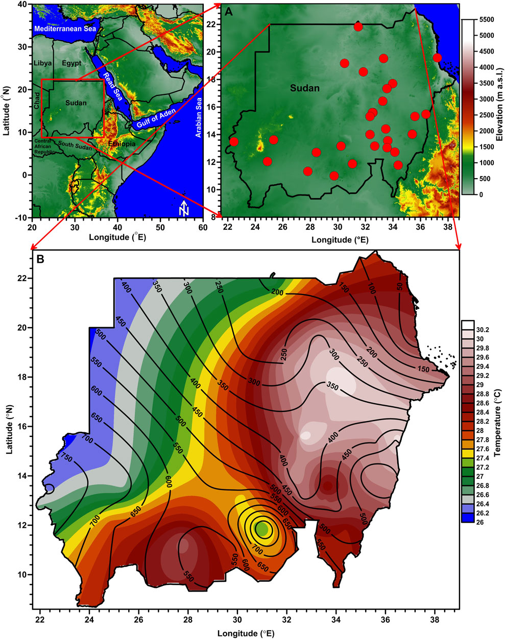
FIGURE 1. The study region’s location, spatial distribution of stations, elevations, and mean temperature. The contour lines in Figure 2B represent the elevation distribution in the study region. The mean temperature is calculated over the period 1981–2010.
The country is unique for its climate diversity, which ranges from dry and semi-arid or arid (desert) over a large area in the north to humid in the south (Elagib and Mansell, 2000). Sudan’s climate is classified into three distinct seasons: summer (wet), winter (dry), and autumn (hot). The spring season is generally not defined in the region. Elagib and Elhag (2011) explain the general characteristics of seasons in Sudan. Because of the dry and arid climatic regime of the study region, the sky is usually clear throughout the year (Diabaté et al., 2004). The northern part of the country has a continental climate, the middle has a savannah climate, and the southern parts have an equatorial climate (Elagib and Elhag, 2011). The heating and cooling processes in the region are generally influenced by dry hot desert and maritime moist air (Burpee, 1972). The monthly variation in wind vector and moisture fluxes at 850 hPa over the study region, illustrated in Figure 2, also provides a general overview of the regional synoptic phenomenon.
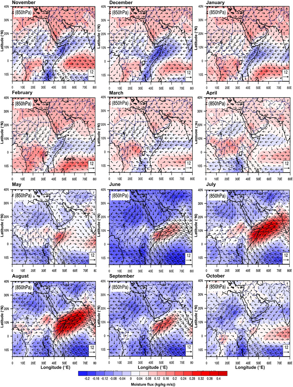
FIGURE 2. Monthly variations in mean wind vector and moisture flux at 850 hPa over the Sudanese region between 1981 and 2010.
The spatial distribution of the mean temperature in Sudan is presented in Figure 1B. The average maximum, minimum, and mean temperatures are 36.32°C, 21.23°C, and 28.77°C, respectively. The month of May has the highest Maximum (40.54°C) and mean (32.82°C) temperatures, but the month of June has the highest minimum temperature (25.40°C). January is the coldest month (Tmax = 31.12°C, Tmin = 12.71°C, and Tmean = 22.92°C). The country is characterized as a high thermal regime region, with high insolation and low evaporation, resulting in low surface pressure throughout the year (Lavaysse et al., 2009). Aside from rainfall, the monthly variability of mean temperature in the region is also linked to dust storm variability (Wilson, 1991). Most parts of the country experience cold and dry weather in December and January (Diabaté et al., 2004; Elagib and Elhag, 2011), with the coldest being July and August in the south (Elagib and Elhag, 2011). Temperatures in the southern parts of the country are mostly uniform and low throughout the year, in contrast to the northern parts (Figure 1B).
The onset of the rainy season in Sudan is highly sporadic with respect to location and timing. Several studies have suggested that the occurrence of rainfall over the study region is correlated to the apparent movement of the Inter Tropical Convergence Zone (ITCZ) (Kyle, 1970; Burpee, 1972; Elagib and Elhag, 2011). The ITCZ is known as a zone of convective rain belt (Sultan and Janicot, 2003), but there is little or no rainfall in its vicinity in the Northern African region due to extreme dryness of the surface air on its pole-ward side and mean tropospheric subsidence aloft (Kyle, 1970; Burpee, 1972). The ITCZ coincides with the minimum surface pressure over the North African land mass: when temperatures are high, a thermal low develops that is elongated in the east-west direction (Burpee, 1972). During the rainy season, the ITCZ is located in the country’s extreme south, which receives the most rainfall.
The spatial distribution of monthly rainfall is presented in Figure 3. Excluding winter, the southernmost part of the country receives the most rainfall. Rainfall is measured from April to October, for the majority of stations in the southernmost part during the summer. However, the amount of rainfall decreases sharply from the south to the country’s extreme northern border during this period (Figure 3). The months of July and August are the wettest in all areas, with the exception of the Red Sea coast. The rainy season in the northern region is found to be relatively short, with rainfall occurring only in August (Figure 3). However, rain is common in winter, especially from October to January in the surrounding area of the Red Sea coast due to littoral effects; but the distribution is quite erratic (Figures 2, 3). Because of the effects of occasional depressions from the southeastern Mediterranean region, the peak amount of rainfall in this study was observed in November (Tsvieli and Zangvil, 2005; Elagib, 2010; Elagib and Elhag, 2011). In response to the effects of westerly winds, noticeable precipitation is also observed in the northern and northeastern parts of the country during the winter months (Figures 2, 3).
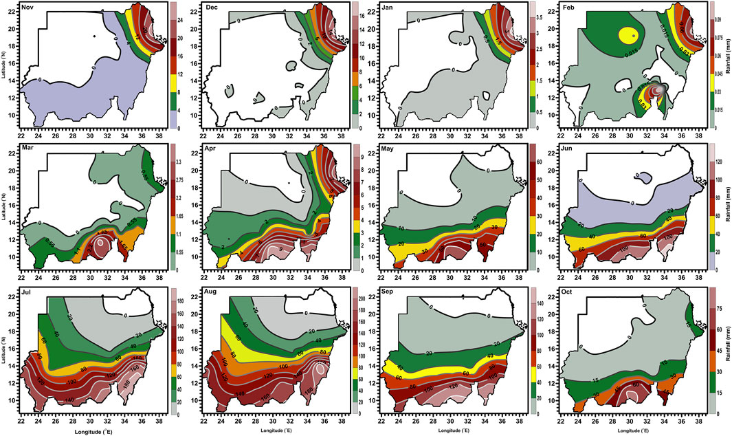
FIGURE 3. The spatial distribution of monthly mean rainfall in Sudan between 1981 and 2010.
Based on previous research by Elagib and Elhag (2011), the classification of seasons in the region is distinct, as we noted earlier. We divided the time in this study into four segments based on meteorological or astronomical classification for ease of comparison with earlier findings from other parts of the world. The amount of solar energy received at the Earth’s surface determines the seasons. This amount is mostly influenced by the angle at which sunlight strikes the surface and the position of the Sun’s shins at any latitude (daylight hours) (Ahrens 2009). Therefore, the months of December, January, and February in this study represent astronomical winter; March, April, and May represent astronomical spring; June, July, and August represent astronomical summer; and September, October, and November represent the astronomical fall (or autumnal). A detailed description of the astronomical categorization from the equator to the pole in both hemispheres is described by Ahrens (2009). It should be noted that this study focuses on the monthly variation in near-surface air temperature gradient and its diurnal range, it does not examine the seasonal variation based on local classification.
3 Data and Methods
3.1 Data and Quality Controls
Thirty years (1981–2010) of monthly mean temperatures (maximum, minimum, and mean), rainfall, cloud cover, and relative humidity data from 29 Sudanese stations (hyper-arid region) were collected from the Sudan Meteorological Authority (SMA), Government of Sudan. This study’s meteorological stations range in elevation from 5 to 850 m above sea level (m a.s.l.). The contour lines in Figure 2B represent the elevation distribution in the study region. The average elevation of the ground is lower in the northern region of the country than in the southern, mountainous region of Darfur (Elagib and Elhag, 2011). Figure 1A depicts the spatial distribution of stations and the elevation of the study region. Table 1 displays information about stations and mean temperatures.
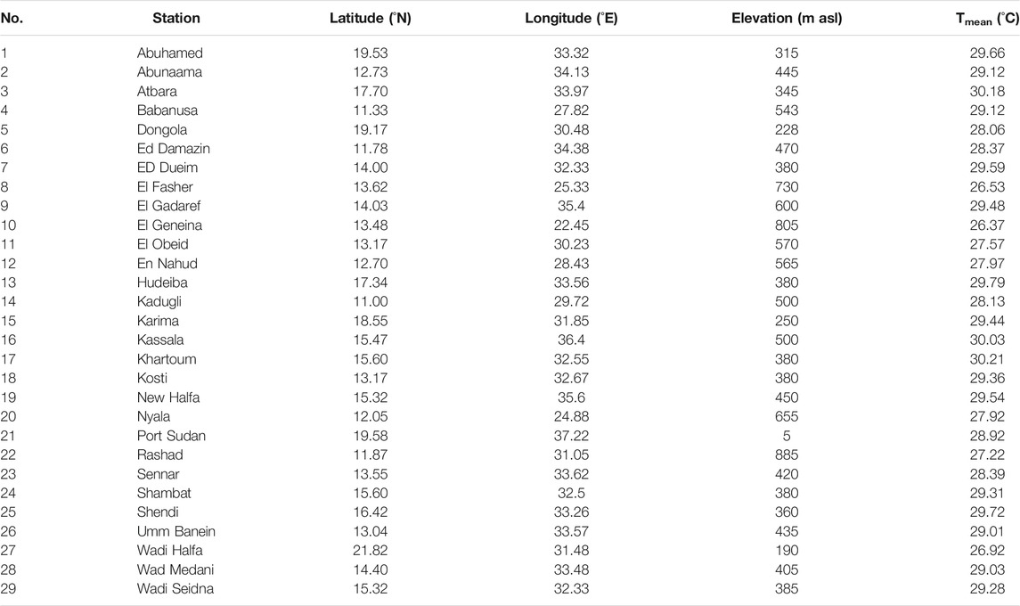
TABLE 1. Information about the stations used in this study.
All 29 stations’ maximum and minimum temperature time series data were subjected to quality control and homogenization. Firstly, all data sets were manually inspected, and any erroneous values, such as minimum temperature greater than the maximum temperature value, were filtered. Then for each data series, Grubb’s method was used to identify unusual values (Grubbs, 1950; Grubbs, 1969). This method helps in the detection of a single outlier in a univariate data set with a reasonably normal distribution. The procedure is described in detail by Kattel et al. (2013) and Kattel and Yao (2013). Outliers were detected in 4.73 percent of the 20,880 (29-station × 12-month × 30-year × 2-maximum and minimum data series) data values. The test statistics and significance values were used as a filter to determine whether these values are outliers or true values. The test statistics for all detected values ranged from 1 to 6. During evaluations, 172 (17.41%) of the 988 outliers had statistically significant (p < 0.05, 0.01, 0.001, and 0.0001). If the test statistic is ≥4 and the significance value p is ≤ 0.0001, the detected values are deemed suspect and removed from the data set. Only 70 (0.33 percent) of the 172 outliers with test statistics of ≥4 and a significance value of p ≤ 0.0001 were removed from the data set.
For all data series, homogeneity tests with respect to time were performed using the well-known criteria of Pettitt (1979), Standard Normal Homogeneity (Alexandersson, 1986); Buishand’s (1982); Von Neumann’s (1941) ratio test . Previous studies by Kattel et al. (2013); Kattel et al. (2019) provide a detailed description as well as standard values to confirm the homogeneity of the data sets. For the investigation, only data sets with significance values greater than 0.01 from this test were used. Based on this criterion, all 29 stations’ data series were found to be homogeneous. Monthly means for each parameter at all stations were calculated from 1981 to 2010 to evaluate temperature gradients and their relationships with other climatic variables.
In addition to the in situ data analysis, we plotted monthly distributions of moisture flux (qv) and wind vector (U, V) for six different pressure levels, 1,000, 925, 850, 700, 600, and 500 hPa, to evaluate its distribution and compare it to the temperature gradient variability over the study region. The moisture flux (qv) was quantified using reanalysis data for the U-wind, V-wind and the specific humidity (q). The National Centers for Atmospheric Research and the National Centers for Environmental Prediction (NCAR/NCEP) provided reanalysis data sets distributed in a 2.5° × 2.5° square grid. Monthly moisture flux (qv) values were also extracted for the above mentioned pressure levels for comparison and analysis. The Open GrADS program was used to compute the moisture flux (qv) and visualize the spatial distribution of moisture in the study region. The analysis covered the same time period, from 1981 to 2010.
3.2 Methods
3.2.1 Estimation of Temperature Gradient
A simple linear regression method is usually used to estimate the near-surface temperature gradient (or lapse rate) value, primarily using two variables (e.g., temperature and elevation). A preliminary analysis of this study shows an inverse relationship between elevation and both latitude (R = −0.74, p = 0) and longitude (−0.59, p = 0.001), possibly due to the north-to-south or southwest distribution of mountains. Individual regression results between temperature and latitudes or elevations (not shown) were also determined to differentiate the elevation and latidutional controls on temperature. We used a simple linear regression model based on a single independent variable in order to obtain the result. Individual model patterns for temperature gradients with elevation or latitude on an annual cycle are identical to multicollinearity results. The linear regression model reveals that the temperature-longitude relationship is relatively weak and variable.
It should be noted that the monthly variation in the magnitude of temperature gradients with latitude is almost identical in both results. Individual models, on the other hand, show that the magnitude of positive and negative gradient (or lapse rate) of temperature with elevation is higher in both summer and winter months. Based on the preliminary evaluations, the elevation effect is likely to be strongest in the summer and the latitude effect is likely to be strongest in the winter. Therefore, we have chosen a model to fit all parameters so as to obtain precise results for evaluations. In addition, the study area is spread across a wide range of geographical coordinate bands of about 14° from south to north and 16° from east to west. Thus, as in previous studies by Kattel et al. (2013), Kattel et al. (2015), and Kattel et al. (2019), a multi-collinearity model was used to determine the best multivariable relationship, primarily to describe the relationship of near-surface air temperature with both elevations and geographical coordinates, per Eq. 1.
The model presented in Eq. 1 is used to investigate the impacts of various simultaneous influences (for example, latitude, longitude, and elevation) on a single dependent variable (temperature). The symbol “
3.2.2 Estimation of
The distinction between wet and dry atmospheric conditions is crucial to understanding the causes of the variation of the lapse rate (or gradient) near the surface (e.g., Kattel et al., 2013), because the atmospheric water-vapor pressure depends only on the vapor temperature. To investigate the moisture present in the atmosphere and its gain or loss, the amount of vapour pressure deficit
Tetens (1930) developed an empirical formula for
The above-mentioned Equation for
The gradients of rainfall, relative humidity, saturation vapor pressure (
4 Results and Analysis
4.1 Evaluations of Co-Linearity, Estimation Strength, and Factors Influencing the Relationship
Table 2 summarizes the results of the multicollinearity analysis, while Table 3 shows the computed error and significance values. In general, the variance inflation factor (VIF) (or
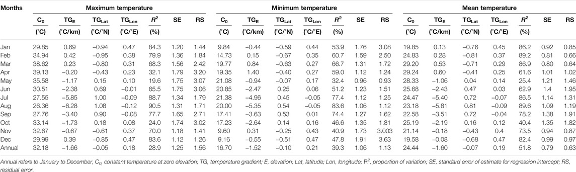
TABLE 2. Results from the multi-collinearity statistical model.
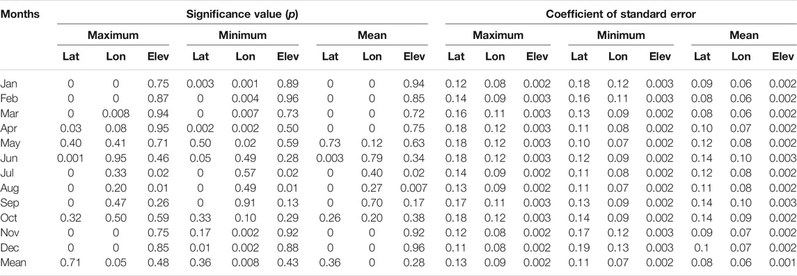
TABLE 3. The coefficient of standard error and the significance value from the multiple regressions.
The significance values derived from the multicollinearity model in this study indicate that the strength of the relationship is more linear between temperature and latitudes than between temperature, elevations, and longitudes, with the exception of the month of May (Table 3). Both latitude and longitude showed a monthly variation in coefficient of standard errors from regression analysis for maximum temperature values between 0.11°C and 0.18°C and 0.08°C and 0.12°C, respectively (Table 3). When compared with geographical coordinates, the coefficient of standard errors for elevation were lower, ranging from 0.002°C to 0.003°C. The errors for the minimum temperatures are also lower than those for the maximum temperatures across all 29 stations. The lower error values observed further imply that the computation results are accurate enough.
Based on the analysis above, the monthly mean square error (MS) of multiple regression is highly variable. The MS for the mean temperature ranges from 0.64°C to 1.95°C. The maximum temperature has larger errors (1.26°C–3.20°C) than the minimum temperature (0.93°C–3.63°C). MS errors for maximum temperatures are highest during the dry months (March to June, September, and October). The highest error (3.20°C) was recorded during the month of April. However, when it comes to minimum temperatures, the winter months has higher MS error values. This season, the highest error value (3.63°C) was recorded in December. In April and December, the highest coefficient values of standard error are also observed for maximum and minimum temperatures (Table 3). In contrast, the lowest MS values are observed in May (0.93°C) for the minimum temperature and in December (1.26°C) for the maximum temperature.
Figures 4A,B depicts the monthly variation in R2 and residual error. The results indicate that a lower (higher) R2 value corresponds to a higher (lower) mean square error. Variation in local topoclimates, surface characteristics, air moisture content, and the synoptic system can all weaken the relationship and cause higher errors (e.g., Harlow et al., 2004; Dobrowski et al., 2009; Kattel et al., 2013; Kattel et al., 2015; Kattel et al., 2019). Furthermore, the R2 value is higher for maximum temperatures (range: 65.5–90.5%) than for minimum temperatures (range: 32.4–83.6%), excluding the months of April, May and October. The lowest R2 values obtained, particularly for minimum temperature, could be attributed to the effects of inversion and local terrain. This effect is more pronounced during the winter months. There is a reduction in R2 value for both maximum (19.6 and 24.0%) and minimum (32.4 and 46.6%) temperatures in May and October (Figure 4; Table 2), presumably because of synoptic disturbances that occur during these transition months (discussed below). Based on the evaluations of R2 and errors, it is also reasonable to explain that local topoclimate influences are stronger for maximum temperatures during April-June, September-October and November, and December-February for the minimum temperatures.
FIGURE 4. Annual variation in the proportion of variation (A) and residual error (B) resulting from multi-coolinearity assessment.
FIGURE 5. Annual cycle of temperature gradient with elevation (A), latitude (B), and longitude (C) over the study region.
4.2 Gradients of Climatic Variables With Elevation and Geographical Coordinates
4.2.1 Temperature Gradient (or Lapse Rate) With Elevation (TGE)
The results of the multi-collenearity evaluations are summarized in Table 2. In this study, the mean monthly values of the near-surface air temperature lapse rate (or gradient) with elevation (TGE) were lower than the value of the free-air moist adiabatic lapse rate (−6.5°C/km). The monthly mean TGE’s values are both positive and negative. August is the month with the highest mean TGE value (−5.81°C/km). It is also the month with the steepest gradient for both maximum (−6.28°C/km) and minimum (−5.35°C/km) temperatures. The TGE values are shallowest (or strong positive) in April, especially for the mean (0.60°C/km) and minimum (1.40°C/km) temperatures, but positive gradient is highest for the maximum temperature (0.69°C/km) in January. During January, March, and December, a positive gradient is observed in maximum temperature with elevation. However, the rest of the year shows negative values (Table 2). The positive gradient values for maximum temperature with elevation range from 0.23 to 0.69°C/km, whereas the negative gradient values range from −6.28 to −0.20°C/km. For February to April, as well as November, the minimum temperature gradient is positive (0.31–1.40°C/km). During the rest of the period, the negative values of minimum TGEs range from −5.35 to −0.44°C/km (Table 2). The study found that TGE values for mean temperature are positive between January and April (ranging from 0.13 to 0.60°C/km), and negative between May and December (ranging from −5.8 to −0.08°C/km).
4.2.2 Temperature Gradients With Geographical Coordinates
In comparison to TGE, the monthly variation in TGLat shows an opposite pattern as shown in Figures 5A,B and Table 2. Latitudinal gradients for maximum (minimum) temperatures range between 0.18°C/°N (0.14°C/°N) in October to −0.95°C/°N (−0.67°C/°N) in February. The mean TGLat value is shown to be positive, close to zero in May (0.04°C/°N), but negative (−0.81°C/°N) in February during cold and dry periods. In January and April, as well as November and December, the mean TGLats are negative. During this period, the gradient value ranges between −0.43 and −0.81°C/°N. TGLats, on the other hand, are positive between May and October, with values ranging from 0.04 to 0.81°C/°N. Temperature gradients with latitude show a similar annual pattern, both for maximum and minimum temperatures. In this study, the negative gradient values range from −0.43 to −0.95°C/°N for maximum and −0.07 to −0.67°C/°N for minimum temperature (Table 2). However, the positive gradient values for maximum and minimum temperatures range from 0.15 to 1.08°C/°N and 0.14 to 0.54°C/°N, respectively. The gradient of temperature with longitude (TGLon) in this study exhibits a pattern similar to the TGE. In contrast, the temperature gradients with longitude are positive for all observation periods except July- September (Figure 5C).
4.2.3 Gradient of Rainfall
Figure 6 shows the monthly variations of mean rainfall and relative humidity (RH) over a 30-year period from all 29 Sudanese stations. August has the most rainfall and the highest humidity (rainfall = 91 mm, RH = 55 percent). However, rainfall in February is almost nil (0.01 mm). The results show that the country experiences low levels of rainfall during the winter months (range: 0.01–0.58 mm), which lasts until the month of March, though some moisture (RH) is observed during this time (RH ∼ 20–35 percent) (Figure 6).
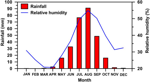
FIGURE 6. The monthly variation in mean rainfall and relative humidity in Sudan between 1981 and 2010.
The Figure 7 and Table 4 present the annual cycle of rainfall gradients with respect to elevation and geographical coordinates. The rainfall gradient with elevation is positive from July to October, with values ranging from 8.67 mm/km to 114.65 mm/km. Furthermore, the positive gradient is highest in August (Figure 7; Table 4). Except for the months of March (1.49 mm/km) and summer and October, the rest of the year shows a negative rainfall gradient. November has the highest negative RGE value (−13.93 mm/km). It should be noted that, with the exception of August, these results are not statistically significant.
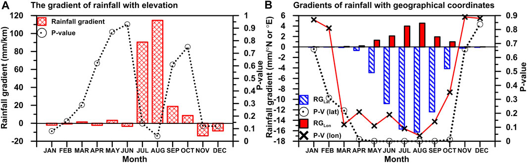
FIGURE 7. Monthly variations in rainfall gradients and their significance values as a function of elevation (A) and geographical coordinates (B).
TABLE 4. Rainfall gradients with elevation and geographical coordinates (latitude and longitude) in the study region.
RGE’s monthly variability is generally consistent with RGLon’s pattern, but the trend is nearly the opposite of RGLat’s (Figures 7A,B). The rainfall gradient with latitude is shown to be negative throughout the observation period, with values ranging from −0.003 to −16.25 mm/°N. There is a strong negative RGLat (−16.25 mm/°N) in August. During the winter, however, RGLat values are almost negligible (not significant). However the results are statistically significant when the RGLat values are steepest, (Figure 7B; Table 4). Except for the month of August, the results for longitude during the entire observation period were not statistically significant.
4.3 Empirical Relationship
Table 5 displays the gradients of es, e, and Δe with elevation and geographical coordinates. A relationship was evaluated empirically between the gradients of temperature and climatic variables (e.g., rainfall, relative humidity, moisture fluxes (qv), es, e, and Δe) to determine the forcing processes (Table 6). The relationship between the annual cycle of mean TGE and rainfall (r = −0.98, p < 0.0001), as well as relative humidity (r = −0.94, p < 0.0001) is strong and statistically significant (Table 6). TGE and rainfall gradient are also found to have a statistically significant but inverse relationship (r = −0.88, p < 0.001). On the other hand, TGEs have a positive relationship with the es GE (r = 0.998, p < 0.0001), e GE (r = 0.31, not significant) and Δe GE (r = 0.82, p < 0.01). In addition, the correlations between maximum and minimum TGE, as well as maximum and minimum es GE, are strongly positive and statistically significant (max: r = 0.99, p < 0.0001; min: r = 0.99, p < 0.0001). These results are consistent with previous studies on the Hindu-Kush and Karakorum mountain ranges by Kattel et al. (2013) and Kattel et al. (2019).
TABLE 5. The gradients of saturation (es), actual vapor pressure (e) and vapor pressure deficit (Δe) in the study region as a function of elevation and geographical coordinates (latitude and longitude).
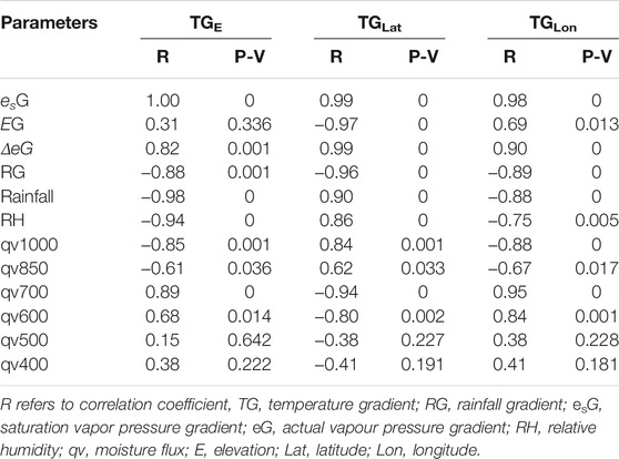
TABLE 6. The coefficients are measured from the correlation evaluation between the gradient of temperatures and climatic variables.
In this study, TGLat and rainfall (r = 0.90, p < 0.0001), as well as relative humidity (r = 0.86, p < 0.0001), were found to be positively related (Table 6). With the exception of the relationship between TGLat and e GLat (r = −0.97, p < 0.0001), the relationships between TGLat and other variables, such as es GLat (r = 0.99, p < 0.0001), Δe GLat (r = 0.99, p < 0.0001) and RGLat (r = -0.96, p < 0.0001), are similar to the TGE observations. TGLon relationships with all variables, on the other hand, are similar to TGE relationships. Mean TGEs and TGLats have a strong and statistically significant inverse relationship (r = −0.93, p < 0.0001). Its relationship with TGLons, on the other hand, is inverse (r = 0.886, p < 0.0001). Therefore, the above results confirm that temperature gradients in the study region are highly sensitive to changes in moisture and local topoclimate, in addition to elevations and geographic coordinates.
5 Discussion
The annual cycle of near-surface temperature gradients (or lapse rates) with both elevation and geographical coordinates in this study has revealed distinct seasonal trends (Figure 5). However, when compared to TGE and TGLon, the pattern for TGlat is inverse. TGE values are steeper during the summer (rainy season) months, but they are shallower (or less strong negative or even positive) during the winter months (Figure 5A). These findings are in agreement with observations from the mid-latitude mountain system (e.g., Rolland, 2003), and partially in agreement with observations from southern slopes of the Karakorum and the Himalayan mountain ranges (e.g., Kattel et al., 2013; Kattel and Yao, 2018; Kattel et al., 2019). The above finding, however, contrasts with findings from the southeastern Tibetan Plateau (SETP), which is located on the northern slopes of the eastern Himalayas (e.g., Kattel et al., 2015). A number of factors determine the thermal conditions in desert regions, including the degree of aridity, latitude, elevation, distance to the coast (Nicholson, 2004). These factors may differ from those that determine the temperature in the Third Pole region’s mountain system. Furthermore, the climates in mountainous areas over the Third Pole region are dominated by tropical cyclones, especially in summer, whereas in this study region, the inter-tropical convergence zone (ITCZ) and equatorial trough dominate the climate (Figure 2). Additionally, the region’s extremely dry and arid climate plays a role in regulating the local thermal regime in comparison to areas over the Third Pole mountain system. As a result, this distinct observation in this study area is not surprising in comparison to the results from the mountain system over the Third Pole and mid-latitude region.
5.1 Forcing Processes for Temperature Gradients Variation Over the Desert Land Surfaces
5.1.1 Variation in Temperature Gradients During Wet and Hot Period
This study demonstrates a strong negative gradient in temperature with increasing elevation during the rainy season (or summer months), but the result is reversed for latitude (Figures 5A,B). Numerous studies from the mid-latitude mountain systems (e.g., Rollend, 2003) have reported similar results, indicating that the steepening of gradients with elevation, particularly during summer, is associated with strong dry convection. The evaluation of various climatic parameters in this study suggests that the forcing mechanisms for TGE variation in summer months are partially consistent with the mechanisms reported in the mid-latitude mountain system. This result, however, is diametrically opposed to those reported in monsoon-dominated areas over the Third Pole regions, where the shallowest TGE value is recorded in rainy summer due to latent heating at higher elevations (e.g., Kattel et al., 2013; Kattel et al., 2015; Kattel and Yao, 2018).
The steepest temperature gradient with elevation (TGEs) in the study region in rainy season (or summer months) corresponds to a period of high solar radiation emissions. The country lies in the tropical belt, which receives a large amount of sensible heat during summer. Combined with the desert land surface, the hot, dry and arid environment creates an extreme thermal environment, particularly in the northern lower elevation regions. Desert land surfaces, in general, cause considerable heat transfer from the ground, as well as mostly ascending air motion in the summer (Barry and Chorley, 2003). As a result of sinking air, lower elevations warm, causing TGE to steepen in this season, especially due to strong dry adiabatic cooling. The high positive TGLat values for this season (Figure 5B) suggest warmer atmospheric conditions at the northern lower elevation station, which agrees with earlier statements. Moreover, increased cooling at higher elevation (or lower latitude) stations in the south and southwest due to excessive rainfall, cloud cover and moisture are responsible for steepening the TGE value during this period (e.g., Leffler, 1981; Kattel and Yao, 2018; Kattel et al., 2019). This is exacerbated by the elevation effect, which is stronger in the region located in the northern lower latitudes. Over the Sudanese region, the upward velocity in a stable atmosphere between pressure levels of 925 and 700 hPa, where the adiabatic term averages, usually result in a cooling process (Lavaysse et al., 2009). This can lead to rain and cloud cover over higher elevation land in the south and southwest, as opposed to the northern and central part of the country (e.g., Figures 2, 3).
The majority of stations in Sudan’s southernmost region experience a sudden drop in air temperature throughout the summer months. This result is associated to elevation, moisture and cloud cover, in addition to the effects of cooling mechanisms (Figure 2). The cooling mechanism in southern Sudan is caused by the ascent of a large parcel of horizontal air, which is simply the congregation of air parcels or masses. This is a common phenomenon on the African continent (Johnson and Morth, 1960). Strong divergence of moisture from the equatorial region at 1,000 and 850 hPa and convergence at 700 hPa (Figure 8) may have triggered precipitation and cloud formation at higher elevations in the south and southwest, possibly induced by cooling mechanisms. The dramatic changes in the relationship between TGE and moisture flux (qv) from 700 hPa (r = 0.89, p < 0.0001) to the higher pressure levels [1,000 hPa (r = −0.85, p < 0.001) and 850 hPa (r = −0.61, p < 0.05)] (Table 6), support the earlier statements. The relationship between TGLat and qv in this study, however, is inverse [e.g., 1,000 hPa (r = 0.84, p < 0.001), 850 hPa (r = 0.62, p < 0.05) and 700 hPa (r = −0.94, p < 0.0001)], which further support the result. The relationship between TGLon and qv is similar to that between TGE and qv, which is consistent with the argument relating the cooling process.
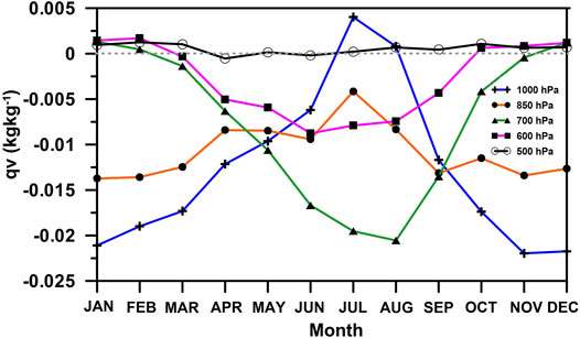
FIGURE 8. Monthly variation in the study region’s area weighted mean moisture flux (qv) at different pressure levels.
Cloud formation and rainfall in this region are also influenced by the northward migration of the Inter Tropical Convergence Zone (ITCZ). The ITCZ is a low pressure trough (also known as a thermal low), which occurs near 18°N and extends east-west near the equator, where the surface northeast and southeast trade winds meet and converge (Burpee, 1972; Flohn et al., 1974; Nicholson, 2004). As these winds converge, warm, moist air is forced upward, resulting in clouds and heavy precipitation. During the summer, the ITCZ can be found in the extreme southernmost part of Sudan, bringing moisture to the region and causing rainfall (Flohn et al., 1974). Thus, our results confirm that the reduced solar heating as well as the increased absorption of heat due to rainfall, moisture, and cloud cover as a result of the ITCZ effects at the south and southwestern higher elevations result in an increased (decreased) TGEs (TGLats) value during the rainy season. Moreover, the intense adiabatic cooling due to the high thermal environment at the northern lower elevation station (or the higher latitude region) enhances the negative (positive) TGEs (TGLats) value. Figure 2 depicts the distribution of U and V, as well as the wind moisture flux (qv) (for a more detailed example in August), which may corroborate the above results.
5.1.2 Variation in Temperature Gradients During Cold and dry Periods
It has been discussed previously that summer months has the greatest negative (positive) value for temperature gradients with elevation (latitude). On the other hand, the result is opposite during cold and dry periods. During the summer, the tropical and subtropical desert regions typically experience very steep temperature gradients, resulting in significant heat transfer from the surface and generally upward motion (Barry and Chorley, 2003). Direct contact with the heated surface causes the air to warm, become more buoyant, and rise. Rising air causes a decrease in atmospheric pressure at the surface, resulting in the formation of a “low”. This upward movement will eventually result in an upper-level outflow (a “high” aloft), which will cause more air to flow into the surface low (Nicholson, 2004; Trapasso, 2004). However, in the winter, air subsidence is associated with high-pressure cells, which are a prominent in desert regions (Barry and Chorley, 2003).
In this study, the shallowest (steepest) values (less negative or even positive) of mean TGEs (TGLats) can be observed from January to April and November to December (Figures 5A,B; Table 2). The mean TGE in this study is close to zero in November, indicating “isothermal” conditions (Figure 5A). Low solar insolation is associated with less strong negative or positive temperature gradients with elevation (TGEs) during dry and cold months, notably in the tropics during winter. Strong positive gradients were found from the individual model results between temperature and elevation regression (not shown). This is mostly owing to latitude effects. The observed strong negative TGLat values during this time period support the above statement (Figure 5B). The observed negligible gradient of TGE, or somewhat “isothermal” conditions during dry months, especially in November, is due to low heat transfer, which is associated with a constant thermal regime across all stations.
Despite a few exceptions, the majority of months in a year cycle in the study region, excluding summer months, record negligible precipitation (Figure 6), indicating a relatively dry period. Additionally, the amount of actual vapor pressure (e) is at its lowest level during this time period. In this time period, the distribution of moisture flux (qv) is inverse in comparison to the summer months, with a particular convergence between pressure levels of 1,000 and 850 hPa (Figure 8). Furthermore, during the cold and dry months, the mean es GE value is found to be shallower (or positive, i.e., close to zero) throughout the observational records (Figure 9A). In this period, however, the result is reversed for es GLat (Figure 9B). The months of December to February are the coldest months in most parts of Sudan, particularly in the north, which is influenced by the continental climate. This could also be one reason for the positive gradients in temperature with elevation in this period. It should be noted that these months also exhibit daytime inversion, which could be attributed to the effects of latitude. The observed reverse patterns of maximum and minimum TGLat in comparison to TGE support the result (Figure 5B).
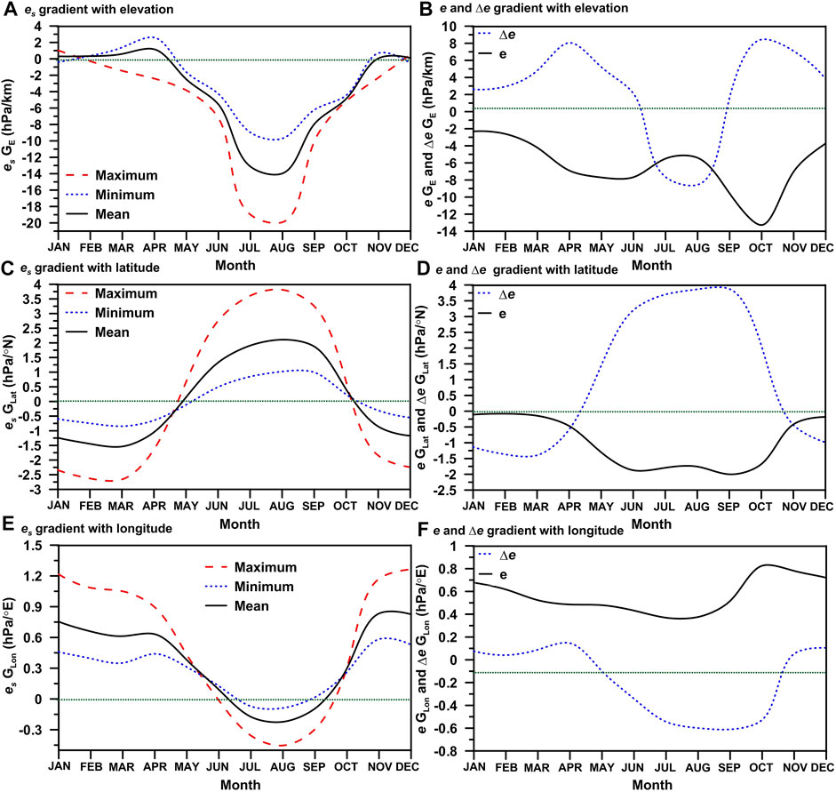
FIGURE 9. The annual cycle of es, e and Δe gradients with elevation (A,B), latitude (C,D) and longitude (E,F) over the study region.
In the winter (December, January, and February), the country receives cold and dry air from the Mediterranean Sea, with pressure levels ranging between 1,000 and 925 hPa. A little moisture flux convergence is observed at 850 hPa in December, particularly along the southern and some middle regions of the country (Figure 2). The atmosphere in the study region is dry from January to April and November to December. The winter months are extremely dry in comparison to the other months. Precipitation is almost negligible throughout the country during winter, with the exception of the northeastern Red Sea coastal belt (Figures 2, 3, 6). In general, rainfall can occur at any time in the coastal region. Nevertheless, it is common during the winter in this study region, and its spatial distribution is quite erratic from October to January, with the peak amount of rainfall occurring in November (Figure 3) (also see Elagib and Mansell, 2000; Elagib and Elhag, 2011).
Rainfall is typically associated with moisture-laden air masses that arrive in Sudan’s coastal region from both the Red Sea and the Arabian Sea. A high amount of moisture convergence was observed at 925 hPa over the Red Sea coast, particularly in November (not shown). A similar pattern can be seen in April, May, and October in the country’s northern and northeastern belts (Figures 2, 10). Furthermore, rainfall occurrences in these months over the study region are linked to the recurrence of occasional depressions along the Eastern Mediterranean Sea (Elagib, 2010). Thus, it is reasonable to conclude that shallower (steeper) TGE (TGLat) values in the study region, mainly in winter, are strongly associated with the effects of latitude, as well as the effects of Mediterranean cold airflow and the prevalence of high rainfall and humidity in the northern and northeastern regions. It is noted that there was a strong inversion during the night in the winter months, when excluding the coastal station in the multicollinearity model (not shown).
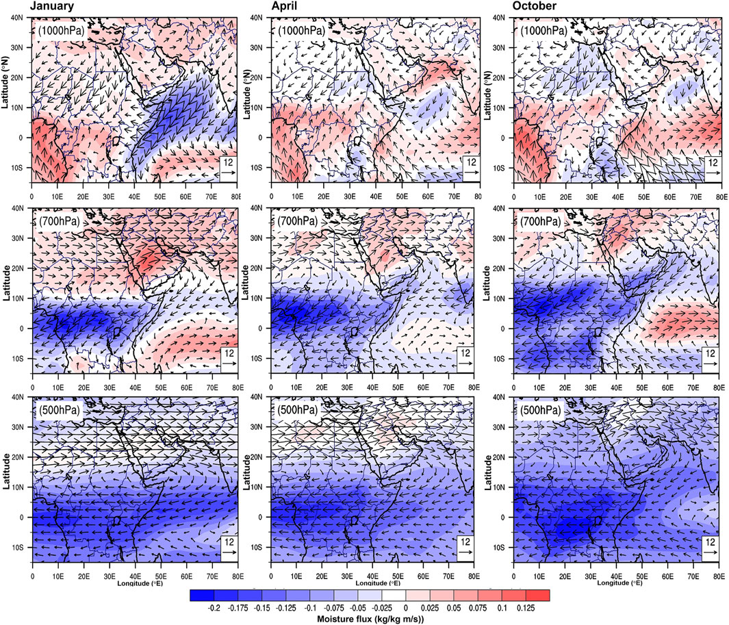
FIGURE 10. The spatial distribution of moisture flux (qv) and wind vector in three different pressure levels over 3 months (e.g., 1,000, 700, and 500 hPa).
5.2 Temperature Gradients Diurnal Range Variation and Extreme Value Observation
The above discussion suggests that seasonal variations in temperature gradients in the study region are closely associated with changes in air moisture content, as well as regional synoptic systems and local topoclimates. In this study, the highest positive value of mean TGE was found in April, whereas its value was strongly negative in August (Figure 5A). The diurnal range of TGE value is recorded as the lowest in contrast to the rest of the year, excluding the months of January, April, July, August, October, and November, as seen in Figure 11A. The minimum diurnal range of TGLat however, is found between the months of April and October (Figure 11B). Apart from the greatest/lowest values of the diurnal range of temperature gradient variations, the month for extreme value observations over the region strongly corresponds with the variation in the Equatorial Trough (ET). In January, April, and October, changing diurnal patterns of temperature gradients are evident, both for elevations and latitudes (see Figures 5A,B), which is also reflected in variations in ET. Similar to the monthly variation in temperature gradients, the moisture flux (qv) also exhibits a similar trend (Figure 8). The study also shows that in summer, the maximum TGE (TGLat) is higher (lower) than the minimum TGE (TGLat), but in winter the result is reversed (Figures 5A,B).
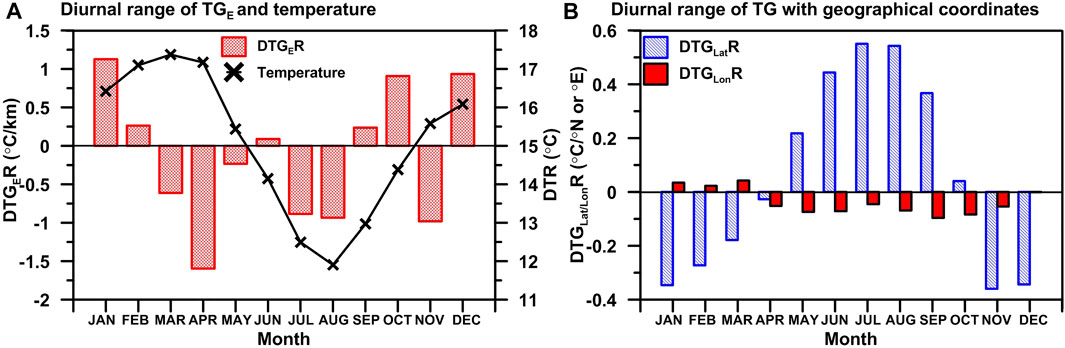
FIGURE 11. Variation in the diurnal temperature range and its gradient with elevation (A) and geographical coordinates (B) in the study region.
5.2.1 Possible Causes for the Extreme Temperature Gradients Observation
This study found that the most unique changes in magnitude of temperature gradients for elevation and latitude occurred in the months of January, April, July, and October (Figures 5A,B). In the study region, these months are referred to as transition months because the annual climate fluctuates considerably during these months. The month of August in summer has the steepest value for TGE (mean = −5.81°C/km; maximum = −6.28°C/km; minimum = −5.35°C/km) (Figure 5A; Table 2). The mean TGE value is also steeper in July (−5.40°C/km), but the magnitude is slightly lower than in August. This month has the highest amounts of rainfall and relative humidity (Figure 6), but their magnitudes are greatest in the southern and southwestern high elevation regions (Figure 3). There is more rainfall in southwestern parts of the country than in the northern or northeastern parts, and this may be due to regional synoptic phenomena (Figure 2). It has been observed that in July and August, water vapor from the south west (south of 10°N) is transported to the Darfur hills (Flohn et al., 1974). A southern component of the ITCZ typically transports water vapor to the convergence zone between latitudes 7°N and 12°N. At 1,000 (also 850) hPa, the divergence of moisture flux from the equator is evident during these months, while the moisture over southern and southern-eastern parts of the country converges at 700 hPa (Figures 2, 8). A convergence of relatively moist air masses usually results in rainfall patterns. This process also reflects the Sun’s seasonal migration (Griffiths, 2004). The observed high amounts of rainfall (Figures 3, 6), particularly at higher elevations, as well as the highest positive (negative) gradient value for rainfall with elevation (latitude) throughout the observation period (Figure 7) are consistent with the above result.
In addition to ITCZ and elevation effects, the steepest value of mean TGEs observed in this study during July and August could be attributed to the dry desert climate found at lower elevations in northern regions (or higher latitudes). There are higher (lower) values of e (Δe) in these months than the rest of the year. Thus, it is also reasonable to explain here that the cooling of moisture received from the surroundings during dry convection in July and August may also result in rainfall (e.g., Kattel et al., 2013; Kattel and Yao, 2018), particularly at higher elevations in the south and southwest. Consequently, the magnitude of TGE may increase further in these months. The magnitudes of es GE (July = −19.00 hPa/km, August = −19.91 hPa/km) and Δe GE (July = −7.65 hPa/km, August = −8.56 hPa/km) are steeper during these months (Figure 9; Table 5), indicating the northern, low-elevation sites receive large amounts of sensible heating. The greatest positive value of mean TGLat, es GLat, and Δe GLat observed in these months throughout the observational record (see Figures 5B, 9B,D) agrees well with the above result. Thus, the steepening of the TGE value in this study during July and August is owing to increased cooling caused by prevailing moisture, rainfall, and cloud cover at the southern lower latitudes due to ITCZ and elevation effects. Furthermore, the strong effects of dry convection caused by receiving large sensible heat due to desert land surface characteristics at the northern lower elevations strengthens the negative TGEs values over the region during these months.
The month of April, noted in this study as a transition month, records the shallowest (highest positive) value of TGE (0.60°C/km) (Figure 5A; Table 2). This month has a very low amount of moisture (Figure 6). In April, the vertical distribution of moisture flux was found to be almost stable (i.e., minimum changes of moisture with changing pressure levels) (Figure 8). Additionally, the value of Δe reaches its peak this month (not shown). The shallowest (highest positive) value of es GE (Figure 9A) is also recorded in April, but the value of Δe GE is shown to be lower (Figure 9B). This suggests that the dry and cold atmospheric period in April corresponds to the highest positive value of mean TGE. The climate of the region is influenced by the cold airflow from the Mediterranean Sea (Figure 10). This synoptic phenomenon intensifies atmospheric cooling over the land surface in higher latitudes or northern lower elevation areas in April, resulting in a sharp reduction (or increase in inversion) in gradient value. However, due to rainfall, the northeastern part of the country is relatively moist this month (Figures 2, 3) as a result of littoral effect. Also, this could lead to a decrease in temperatures over northeastern areas, which might help to boost positive TGE values (or increase inversions). In this study, the temperature gradient with elevation (latitude) steepens (shallows) consistently from April to September (Figure 5). The situation is almost identical for es, e and Δe gradient variations (Figure 9). A similar monthly feature in moisture flux variation is also noticed (Figure 8). Evidence also suggests that the monthly variation in TG over the region is strongly related to the variation in moisture content in the air.
The terms “high Sun” and “low Sun” in summer and winter, respectively, are used to describe reasonably changing temperatures in the tropics, (Griffiths, 2004). In this study, the steepest (strongly negative) value for TGLat was observed in February (Figure 5B). The mean es GLat and Δe GLat values are steepest in the months of February and March (Figures 9C,D). The mean es GE is extremely low in February (Figure 9A). In this study, however, the e GLat is negligible during the winter compared to the other seasons (Figure 9D). In February, in addition to the effects of the low Sun, the influence of the Mediterranean cold and dry air on higher latitudes is stronger. The magnitude of the wind vector component is found to be greater in this month than in April (Figure 2), which agrees with the result. Moreover, the result shows that the value of TGLat in October is close to zero (0.16°C/°N) (Figure 5B; Table 2). This month has the highest positive value for Δe GE, which is nearly identical to the observation in April (Figure 9B). In October, the Δe value is higher, but the magnitude is lower than in April. In addition, the magnitude of e GE is greatest in this month compared to the rest of the period (Figure 9B). Thus, the result suggests that the forcing process in October is similar to that in April, but moisture convergence in this month is expected to be greater at higher pressure levels than in April (Figure 10). This could be a factor in the occurrences of rainfall in the north and northeastern lower elevation region, causing TGE (TGLat) values to shallow (steepen) further this month. The high amount of rainfall and relative humidity observed in October compared to April (Figures 3, 6), agrees well with the result. It is therefore reasonable to conclude that the variation in extreme values of temperature gradient in the study region are influenced by the equatorial trough, as well as moisture, regional synoptic phenomena, and local topo-climate.
5.2.2 Forcing Processes for Temperature Gradient’s Diurnal Range Variation
Deserts are characterized by an extreme thermal environment, and by large changes in temperature between day and night throughout the year (Griffiths, 2004; Nicholson, 2004). The scant of cloud cover and low moisture content in the air in subtropical desert regions results in a regime of high solar insolation and surface temperature. The diurnal range of TGE (TGEmax–TGEmin) in the study region is found to be greater (negative) during the months of July (−0.89°C/km) and August (−0.93°C/km) (Figure 11A). The TGLat results are comparable, but the diurnal range differences (TGLatmax−TGLatmin) are positive throughout the observation period (Figure 11B). The greatest diurnal range for both TGE and TGLat observed in this study is associated with high solar insolation during the day and intense radiative cooling at night. In July and August, we observe steeper (shallower or positive) values of TGEs (TGLats) during the day than at night (Figures 5A,B; Table 2), which is consistent with the aforesaid result. Except for coastal belts, precipitation is minimal in the northern parts of the country during these months (Figure 3). The northern parts of the country also receive significant solar heating in July and August (Burpee, 1972). This could explain why we observed stronger positive TGLat during the day than at night in this study (see Figure 5B).
In general, the dryness of the soil and the lack of dense vegetation cover to absorb and redistribute solar radiation near the ground raise the temperature in desert regions (Nicholson, 2004). Heat is confined to the surface of the dry ground due to the deeper layers of soil; with depth into the ground as well as height above it, temperatures decrease rapidly. The observed steepest value (negative) of es GE during the day versus night in July (−19.00 hPa/km) and August (−19.91 hPa/km) (Figure 9A), clearly explains the above statements. The positive maximum TGLat (or es GLat) is greater than the negative minimum TGLat (or es GLat) in this month (Figures 5B, 9C), which further supports the result. The northern lower elevation atmosphere warms as a result of the effects of high solar insolation and a dry desert climatic regime, resulting in strong dry adiabatic cooling during the day. Furthermore, during the day, high amounts of rainfall, relative humidity, and cloud cover reduce solar insolation, favoring cooling of air near the surface at higher elevations in the south and southwest. As a result of these two processes, the temperature gradient values in the region are accentuated; therefore, the daytime TGE (TGLat) value is steepest (shallowest) in July and August in the region.
In the summer, radiative cooling at low elevations exacerbated by desert surface characteristics and warming at higher elevations caused by inverted lapse rates reduce TGE values at night. Increased temperatures at higher elevations at night due to increased cloud cover, rain, and relative humidity also reduce the minimum TGEs value (less strong negative than the maximum TGEs) in this period. There is no subsurface thermal reservoir due to the concentration of heat at the surface in the desert region (Nicholson, 2004). Moreover, where there is little or no vegetation cover, at night the surface cools extremely rapidly and efficiently. Generally, clear skies and dry air near the ground allow the majority of heat accumulated during the day to escape to the upper atmosphere at night (90% as compared to 50% in humid regions). This accentuates the nighttime cooling (Nicholson, 2004; Kattel et al., 2013; Kattel and Yao, 2018). The high summer values of positive minimum TGLat, as illustrated in Figure 5A, are coherent with the aforementioned statements. Significant differences in DTR values, such as higher (lower) at lower (higher) elevations or higher (lower) latitudes (not shown), further support the result.
The lowest TGE diurnal range values were found in June (0.09°C/km) and September (0.23°C/km) in this study (Figures 5A, 11A). However, there is a discrepancy with the result of TGLat (Figures 5B, 11B). Dust winds could be responsible for the lowest DTGER in these months. During hazy conditions, solar heating can be reduced during the day, while warming at night can be increased at lower elevations (or at higher latitudes) due to trapped released heat. This could be the reason for lower DTGER values in the study region in June and September. Diabaté et al. (2004) found a low clearness index along the northern African desert region during these months, which may support the above statements. These months also have lower DTR range values than July and August, particularly at the lower elevation station. A decrease in DTGR value may also be associated with increasing and decreasing cloud cover at higher elevations during the day and night, respectively (e.g., Kattel et al., 2013).
The value of the diurnal range for TGE is highest in the month of April (Figure 11A). This month, the minimum TGE value is considerably higher (1.40°C/km) than the maximum TGE (−0.20°C/km). In general, DTR values in desert regions can be extreme, sometimes exceeding 20°C (Griffiths, 2004). This extreme condition could be caused by the high amounts of radiation and sunshine hours. During the month of April, the majority of the stations in this study record DTR values above 18°C. Hence, the greatest diurnal range of TGE observed during this month is associated with strong radiative heating during the day and significant radiative cooling during the night. The observed shallowest value for minimum es GE in April (strongly positive) (1.6 hPa/km) compared to maximum es GE (−2.41 hPa/km) (Figure 9A; Table 5) is in good agreement with the result. Additionally, the highest positive value of Δe GE (Figure 9B; Table 5) further supports the above statement.
In April, the daytime TGE value is relatively weak, indicating somewhat isothermal conditions. This month, however, the TGLat difference between day (−0.43°C/°N) and night (−0.40°C/°N) is stable (Figures 5B, 11B; Table 2). TGLat had a similar result in October. The diurnal pattern of TGLat in this study is reversed from April to October (e.g., the increasing rate of maximum temperature with latitude is greater than the increasing rate of minimum temperature with latitude). The result for es GLat is similar, but the magnitude of the diurnal range varies slightly in April and October. Thus, evidence clearly indicates the effects of regional synoptic phenomena in addition to the effects of moisture variability. The amount of moisture is higher in October than in April (see Figure 10), also supports this notion. The variability of the regional climate system may also have played a role in this distinct observation, since April and October are also transition months, and the climate of these months is primarily influenced by the equatorial trough, as well as the westerly winds.
The mean TGE value is relatively stable during the winter months (DJF) and in March during the astronomical spring months. For TGLat, the result is almost comparable (Figure 5B). In May, the diurnal range of TGE over the study region is negligible (Figures 5A, 11A; Table 2). This month, the mean TGLat value is close to zero (0.04°C/°N). The diurnal range of es GLat is also found to be negligible in this month (Figure 9C). It is worth noting that the value of es GLat in May is slightly greater than the value in October. The climate of the study region is relatively dry, and rainfall is almost negligible during this time period. During the winter months, relatively small amounts of moisture convergence can be observed along the Red Sea coast (northeast part) and in the central western part of the country; this leads to a decrease in daytime air temperatures at lower elevations.
During the winter, the most frequent heat lows (West Africa) occur over the eastern Central African Republic (8°N, 20°E), mainly along the southeastern edge of the Darfur mountains (Lavaysse et al., 2009). In March, the elongated heat trough is moving slightly to the north, which is linked to the solar radiation moving northward. The western African heat low over the Sudanese region in November takes the form of an elongated heat trough, the same as in March. Finally, the heat low position in December is similar to that in January. Therefore, in addition to the synoptic phenomenon, the region’s diurnal TGE range variation can also be attributed to the variation in heat trough, in addition to the effects of strong radiative cooling and inversion, especially during cold and dry periods. The observed reverse pattern of TGLat (Figure 5B), and the greatest DTR range recorded in this period (not shown), support our conclusion.
The maximum TGLat is found to be steeper (strongly negative) between November and March (Figure 5B). TGE, on the other hand, has the opposite effect (Figure 5A). Results suggest that the atmosphere along the northern lower elevation stations is relatively cooler than that along southern higher elevation stations during the day. The cold airflow from the Mediterranean Sea combined with the low Sun can be attributed to this result. Moreover, the dampening effect of dust haze/storms is attributed to daytime cooling in the northern part of the country during the dry season (Elagib, 2010). Strong northerly winds blow for much of the long dry season, causing dust storms in the study region and greatly reducing visibility and Sun effects. As a result, sudden temperature drops occur (Wilson, 1991). The observed inverse TGLat during the day as previously discussed, agrees well with the above-mentioned result. The clearness index (m) is found to be greater than 0.70 in the boreal winter, particularly from November to March. With the exception of December, when dust winds occur and reduce the clearness index (m) to 0.66, the value reaches a maximum of 0.74 in February (Diabaté et al., 2004). Except for the month of June, the clearness index (m) is always greater than 0.60 during the rest of the year. During this month, the clearness index in the study region is generally 0.55, owing to heavy dust winds, which also corroborates the aforementioned results.
6 Conclusion
This paper investigated for the first time the monthly, and diurnal characteristics of temperature gradients with elevation and geographical coordinates over tropical desert land surfaces using a 30-year (1981–2010) climatic data set collected at 29 Sudanese stations. Gradients were computed using the multicolinearity technique, and additional forcing mechanisms were determined by establishing empirical relationships between gradients of temperature and gradients of other climatic variables (e.g. es, e, Δe, rainfall, RH and qv). The proportion of variations (R2) and errors were evaluated to determine the accuracy of the results and also to determine the possible effects of topo-climate and other local/regional factors on the relationship.
This study demonstrates TGE’s distinct annual cycle, with the steepest value (greatest negative) occurring during the warm and rainy period (or summer months) and the shallowest (less strong negative or even positive) value occurring during the cold winter or dry months. However, the result is reversed for TGLat. Reduced solar heating during the day and increased heat absorption at night due to increased rainfall, humidity, and cloud cover associated with the ITCZ, as well as elevation effects on lower latitudes in the south and southwest, are likely to contribute to the steepest (shallowest) TGE (TGLat) values observation during wet months (or summer). In these months, a combination of intense adiabatic cooling (inversion) during the day and less inversion (cooling) effect during the night resulted in further increases (decreases) in mean TGEs (TGLats) values.
The shallowest value of mean TGE occurs during the cold and dry months and even has positive values during the winter months, as well as the months of March and April in this period. For TGLat, the result is reversed. Low solar insolation during the day, combined with the effects of Mediterranean cold air flow, inversion and radiative cooling during the night at northern lower elevations (or higher latitudes), results in the shallowest or even positive values for mean TGE and steepest values for TGLat during cold and dry periods. The amount of rainfall and moisture at lower elevations in the north and northeast causes a less strong negative or positive (strong negative) gradient value for TGE (TGLat) during the winter months. During these months, this is also contributes for weakening the inversion effect during the night.
In addition to the highest and lowest gradient values, the dramatic variation in maxima and minima diurnal range for temperature gradients is observed during transition months (e.g., January, April, and October), which strongly coincides with the variation in the equatorial trough, moisture, as well as diurnal variation in radiative energy. Again, the considerable effects of desert land surfaces, Mediterranean cold air flow, and ITCZ further strengthen the TG magnitude and diurnal range over the region. The contrasting features of TG, most notably the gradient of temperature with elevation in this study from the mid-latitudes to mountainous areas over the third pole, are due to distinct differences in local and regional climate, as well as variation in topography, land surfaces, microclimate, and geographical coordinates.
The study’s findings add value to temperature variation analysis in the desert region, and it also suggests expanding the region’s monitoring network stations. More fine and precise scale variation of TG is required using in situ data sets in combination with the use of operational environmental satellites in remote regions. Nevertheless, the study’s findings can be effectively used by the region’s hydro-climate research community to more accurately monitor the variation of climate variables, as well as to better understand the country’s basic climatic characteristics and processes. In addition, the results are applicable to hydro-climatic, ecological, and agricultural modeling, particularly in quantifying the temperature field in the desert region.
Data Availability Statement
The data analyzed in this study is subject to the following licenses/restrictions: The original contributions presented in the study are included in the article material. Requests to access these datasets should be directed to the data are not publicly available, further inquiries can be directed to the corresponding author.
Author Contributions
All authors listed have made a substantial, direct, and intellectual contribution to the work and approved it for publication.
Funding
The work is supported by the Second Tibetan Plateau Scientific Expedition and Research Program (STEP), Grant No. 2019QZKK0201, and the Chinese Academy of Sciences’ Strategic Priority Research Program, Grant No. XDA20100300. DK is financially supported by the Chinese Academy of Sciences (CAS) President’s International Fellowship Initiative for Visiting Scientist (Grant No. 2016VEB013).
Conflict of Interest
The authors declare that the research was conducted in the absence of any commercial or financial relationships that could be construed as a potential conflict of interest.
Publisher’s Note
All claims expressed in this article are solely those of the authors and do not necessarily represent those of their affiliated organizations, or those of the publisher, the editors and the reviewers. Any product that may be evaluated in this article, or claim that may be made by its manufacturer, is not guaranteed or endorsed by the publisher.
Acknowledgments
The authors thank the Sudan Meteorological Authority (SMA), Government of Sudan, for providing the data. We also thank Christopher Andrew Beale for the editing of the manuscript.
References
Ahrens, C. D. (2009). Meteorology Today: An Introduction to Weather, Climate and the Environment. 9th edn1st edn 2002. United State of America: Brooks Cole Publication Company, 57–64.
Albaba, I. (2014). The Effects of Slope Orientations on Vegetation Characteristics of Wadi Alquf forest reserve (WAFR) West Bank-Palestine. Int. J. Agric. Soil Sci. 2 (7), 118–125.
Alexandersson, H. (1986). A Homogeneity Test Applied to Precipitation Data. J. Climatol. 6, 661–675. doi:10.1002/joc.3370060607
Barry, R. G., and Chorley, R. J. (2003). Atmosphere, Weather and Climate. 8th edn. 1st edn, 1968. London: Routledge, 25 pp.
Bennie, J. J., Wiltshire, A. J., Joyce, A. N., Clark, D., Lloyd, A. R., Adamson, J., et al. (2010). Characterising Inter-annual Variation in the Spatial Pattern of thermal Microclimate in a UK upland Using a Combined Empirical-Physical Model. Agric. For. Meteorology 150, 12–19. doi:10.1016/j.agrformet.2009.07.014
Blandford, T. R., Humes, K. S., Harshburger, B. J., Moore, B. C., Walden, V. P., and Ye, H. (2008). Seasonal and Synoptic Variations in Near-Surface Air Temperature Lapse Rates in a Mountainous Basin. J. Appl. Meteorology Climatology 47, 249–261. doi:10.1175/2007jamc1565.1
Bolstad, P. V., Swift, L., Collins, F., and Régnière, J. (1998). Measured and Predicted Air Temperatures at basin to Regional Scales in the Southern Appalachian Mountains. Agric. For. Meteorology 91, 161–176. doi:10.1016/s0168-1923(98)00076-8
Brunt, D. (1939). Physical and Dynamical Meteorology. 2nd ed. London: Cambridge University Press, 103.
Buishand, T. A. (1982). Some Methods for Testing the Homogeneity of Rainfall Records. J. Hydrol. 58, 11–27. doi:10.1016/0022-1694(82)90066-x
Burpee, R. W. (1972). The Origin and Structure of Easterly Waves in the Lower Troposphere of North Africa. J. Atmos. Sci. 29 (1), 77–90. doi:10.1175/1520-0469(1972)029<0077:toasoe>2.0.co;2
Cramer, O. P. (1972). Potential Temperature Analysis for Mountainous Terrain. J. Appl. Meteorol. 11, 44–50. doi:10.1175/1520-0450(1972)011<0044:ptafmt>2.0.co;2
Diabaté, L., Blanc, P., and Wald, L. (2004). Solar Radiation Climate in Africa. Solar Energy 76 (6), 733–744.
Diaz, H. F., and Bradley, R. S. (1997). Temperature Variations during the Last century at High Elevation Sites. Clim. Chang. 36, 253–279. doi:10.1023/A:1005335731187
Dobrowski, S. Z., Abatzoglou, J. T., Greenberg, J. A., and Schladow, S. G. (2009). How Much Influence Does Landscape-Scale Physiography Have on Air Temperature in a Mountain Environment? Agric. For. Meteorology 149, 1751–1758. doi:10.1016/j.agrformet.2009.06.006
Elagib, N. A. (2010). Trends in Intra- and Inter-annual Temperature Variabilities across Sudan. Ambio 39 (5-6), 413–429. doi:10.1007/s13280-010-0042-3
Elagib, N. A., and Elhag, M. M. (2011). Major Climate Indicators of Ongoing Drought in Sudan. J. Hydrol. 409 (3–4), 612–625. doi:10.1016/j.jhydrol.2011.08.047
Elagib, N. A., and Mansell, M. G. (2000). Recent Trends and Anomalies in Mean Seasonal and Annual Temperatures over Sudan. J. Arid Environments 45 (3), 263–288. doi:10.1006/jare.2000.0639
Flohn, H., Henning, D., and Korff, H. C. (1974). Possibilities and Limitations of a Large-Scale Water Budget Modification in the Sahel-Sudan belt of Africa. Met. Rdsch. 27, 97–100.
Good, E. J. (2016). An In Situ-based Analysis of the Relationship between Land Surface "skin" and Screen-Level Air Temperatures. J. Geophys. Res. Atmos. 121, 8801–8819. doi:10.1002/2016JD025318
Griffiths, J. F. (2004). “African Climate,” in Encyclopedia of World Climatology. Editor J. E. Oliver (The Netherlands: Springer).
Grubbs, F. E. (1969). Procedures for Detecting Outlying Observations in Samples. Technometrics 11 (1), 13–14. doi:10.1080/00401706.1969.10490657
Grubbs, F. E. (1950). Sample Criteria for Testing Outlying Observations. Ann. Math. Statist. 21, 27–58. doi:10.1214/aoms/1177729885
Harlow, R. C., Burke, E. J., Scott, R. L., Shuttleworth, W. J., Brown, C. M., and Petti, J. R. (2004). Research Note:Derivation of Temperature Lapse Rates in Semi-arid South-Eastern Arizona. Hydrol. Earth Syst. Sci. 8 (6), 1179–1185. doi:10.5194/hess-8-1179-2004
Jain, S. K., Goswami, A., and Saraf, A. K. (2008). Determination of Land Surface Temperature and its Lapse Rate in the Satluj River basin Using NOAA Data. Int. J. Remote Sensing 29 (11), 3091–3103. doi:10.1080/01431160701468992
Jin, M., Dickinson, R. E., and Vogelmann, A. M. (1997). A Comparison Of CCM2/BATS Skin Temperature And Surface Air Temperature With Satellite And Surface Observations. J. Climate 10, 1505–1524.
Johnson, D. H., and Morth, H. T. (1960). “Forecasting Research in East Africa,” in Tropical Meteorology in Africa. Editor D. J. Bargman (Nairobi: Munitalp Foundation), 56–137.
Kattel, D. B., Yao, T., and Panday, P. K. (2017). Near-surface Air Temperature Lapse Rate in a Humid Mountainous Terrain on the Southern Slopes of the Eastern Himalayas. Theor. Appl. Climatol. 132, 4. doi:10.1007/s00704-017-2153-2
Kattel, D. B., and Yao, T. (2013). Recent Temperature Trends at Mountain Stations on the Southern Slope of the central Himalayas. J. Earth Syst. Sci. 122 (1), 215–227. doi:10.1007/s12040-012-0257-8
Kattel, D. B., and Yao, T. (2018). Temperature-topographic Elevation Relationship for High Mountain Terrain: an Example from the southeastern Tibetan Plateau. Int. J. Climatol. 38, e901–e920. doi:10.1002/joc.5418
Kattel, D. B., Yao, T., Ullah, K., and Rana, A. S. (2019). Seasonal Near-Surface Air Temperature Dependence on Elevation and Geographical Coordinates for Pakistan. Theor. Appl. Climatol. 138, 1591–1613. doi:10.1007/s00704-019-02899-5
Kattel, D. B., Yao, T., Yang, K., Tian, L., Yang, G., and Joswiak, D. (2013). Temperature Lapse Rate in Complex Mountain Terrain on the Southern Slope of the central Himalayas. Theor. Appl. Climatol. 113, 671–682. doi:10.1007/s00704-012-0816-6
Kattel, D. B., Yao, T., Yang, W., Gao, Y., and Tian, L. (2015). Comparison of Temperature Lapse Rates from the Northern to the Southern Slopes of the Himalayas. Int. J. Climatol. 35 (15), 4431–4443. doi:10.1002/joc.4297
Kitoh, A. (1997). Mountain Uplift and Surface Temperature Changes. Geophys. Res. Lett. 24 (2), 185–188. doi:10.1029/96gl03953
Komatsu, H., Hashimoto, H., Kume, T., Tanaka, N., Yoshifuji, N., Otsukik, K., et al. (2010). Modeling Seasonal Changes In The Temperature Lapse Rate In A Northern Thailand Mountainous Area. J. Appl. Meteorol. Climatol. 49, 1233–1246.
Kyle, A. C. (1970). Longitudinal Variations of Large-Scale Vertical Motion in the Tropics. Cambridge: Department of Meteorology, M. I. T. S.M. Thesis.
Lavaysse, C., Flamant, C., Janicot, S., Parker, D. J., Lafore, J. P., Sultan, B., et al. (2009). Seasonal Evolution of the West African Heat Low: a Climatological Perspective. Clim. Dyn. 33 (2-3), 313–330. doi:10.1007/s00382-009-0553-4
Leffler, R. J. (1981). Estimating Average Temperatures on Appalachian Summits. J. Appl. Meteorol. 20, 637–642. doi:10.1175/1520-0450(1981)020<0637:eatoas>2.0.co;2
Lian, X., Zeng, Z., Yao, Y., Peng, S., Wang, K., and Piao, S. (2017). Spatiotemporal Variations in the Difference between Satellite‐observed Daily Maximum Land Surface Temperature and Station‐based Daily Maximum Near‐surface Air Temperature. J. Geophys. Res. Atmos. 122 (4), 2254–2268. doi:10.1002/2016jd025366
Lookingbill, T., and Urban, D. L. (2003). Spatial Estimation of Air Temperature Differences for Landscape-Scale Studies in Montane Environments. Agric. For. Meteorology 114, 141–151. doi:10.1016/s0168-1923(02)00196-x
Magnus, G. (1844). Versuche über die Spannkräfte des Wasserdampfs. Ann. Phys. Chem. 137, 225–247. doi:10.1002/andp.18441370202
Mahrt, L. (2006). Variation of Surface Air Temperature in Complex Terrain. J. Appl. Meteorol. Climatol. 45, 1481–1493. doi:10.1175/jam2419.1
Marotzke, J., and Forster, P. M. (2015). Forcing, Feedback and Internal Variability in Global Temperature Trends. Nature 517 (7536), 565–570. doi:10.1038/nature14117
Marshall, S. J., Sharp, M. J., Burgess, D. O., and Anslow, F. S. (2007). Near-surface-temperature Lapse Rates on the Prince of Wales Icefield, Ellesmere Island, Canada: Implications for Regional Downscaling of Temperature. Int. J. Climatol. 27, 385–398. doi:10.1002/joc.1396
McCutchan, M. H., and Fox, D. G. (1986). Effect of Elevation and Aspect on Wind, Temperature and Humidity. J. Clim. Appl. Meteorol. 25, 1996–2013. doi:10.1175/1520-0450(1986)025<1996:eoeaao>2.0.co;2
Minder, J. R., Mote, P. W., and Lundquist, J. D. (2010). Surface Temperature Lapse Rates over Complex Terrain: Lessons from the Cascade Mountains. J. Geophys. Res. 115, D14122. doi:10.1029/2009JD013493
Mokhov, I. I., and Akperov, M. G. (2006). Tropospheric Lapse Rate and its Relation to Surface Temperature from Reanalysis Data. Izv. Atmos. Ocean. Phys. 42 (4), 430–438. doi:10.1134/S0001433806040037
Nicholson, S. E. (2004). “Deserts,” in Encyclopedia of World Climatology. Editor J. E. Oliver (The Netherlands: Springer), 324.
O’brien, R. M., and Robert, M. (2007). A Caution Regarding Rules of Thumb for Variance Inflation Factors. Qual. Quant. 41 (5), 673–690. doi:10.1007/s11135-006-9018-6
Pelletier, J. D., Barron‐Gafford, G. A., Gutiérrez‐Jurado, H., Hinckley, E. L. S., Istanbulluoglu, E., McGuire, L. A., et al. (2018). Which Way Do You Lean? Using Slope Aspect Variations to Understand Critical Zone Processes and Feedbacks. Earth Surf. Process. Landforms 43 (5), 1133–1154. doi:10.1002/esp.4306
Pérez Díaz, C. L., Lakhankar, T., Romanov, P., Muñoz, J., Khanbilvardi, R., and Yu, Y. (2015). Near-surface Air Temperature and Snow Skin Temperature Comparison from CREST-SAFE Station Data with MODIS Land Surface Temperature Data. Hydrol. Earth Syst. Sci. Discuss. 12, 7665–7687. doi:10.5194/hessd-12-7665-2015
Pettitt, A. N. (1979). A Non-parametric Approach to the Change-point Problem. Appl. Stat. 28, 126–135. doi:10.2307/2346729
Rolland, C. (2003). Spatial and Seasonal Variations of Air Temperature Lapse Rates in alpine Regions. J. Clim. 16, 1032–1046. doi:10.1175/1520-0442(2003)016<1032:sasvoa>2.0.co;2
Schneider, S. H., and Dickinson, R. E. (1974). Climate Modeling. Rev. Geophys. Space Phys. 12, 447–493.
Shen, S., and Leptoukh, G. G. (2011). Estimation of Surface Air Temperature over central and Eastern Eurasia from MODIS Land Surface Temperature. Environ. Res. Lett. 6 (4), 045206. doi:10.1088/1748-9326/6/4/045206
Sultan, B., and Janicot, S. (2003). The West African Monsoon Dynamics. Part II: The “Preonset” and “Onset” of the Summer Monsoon. J. Clim. 16, 3407–3427. doi:10.1175/1520-0442(2003)016<3407:twamdp>2.0.co;2
IPCC (2013). “Climate Change 2013. The Physical Science Basis,” in Contribution of Working Group I to the Fifth Assessment Report of the Intergovernmental Panel on Climate Change. Editor T. F. Stocker (New York: Cambridge Univ. Press).
Toro Guerrero, F. J. D., Hinojosa-Corona, A., and Kretzschmar, T. G. (2016). A Comparative Study of NDVI Values between North- and South-Facing Slopes in a Semiarid Mountainous Region. IEEE J. Sel. Top. Appl. Earth Observations Remote Sensing 9 (12), 5350–5356. doi:10.1109/jstars.2016.2618393
Trapasso, L. M. (2004). “Temperature Distribution,” in Encyclopedia of World Climatology. Editor J. E. Oliver (The Netherlands: Springer), pp711.
Tsvieli, Y., and Zangvil, A. (2005). Synoptic Climatological Analysis of ‘wet' and ‘dry' Red Sea Troughs over Israel. Int. J. Climatol. 25 (15), 1997–2015. doi:10.1002/joc.1232
Von Neumann, J. (1941). Distribution of the Ratio of the Mean Square Successive Difference to the Variance. Ann. Math. Statist. 12, 367–395. doi:10.1214/aoms/1177731677
Whiteman, C. D., Bian, X., and Zhong, S. (1999). Wintertime Evolution of the Temperature Inversion in the Colorado Plateau Basin. J. Appl. Meteorol. 38, 1103–1117. doi:10.1175/1520-0450(1999)038<1103:weotti>2.0.co;2
Keywords: temperature gradients, extreme values, diurnal variation, monthly variation, Controls, tropical desert regions, Sudan
Citation: Kattel DB, Salih HAM, Yao T and Ullah K (2022) Near-Surface Air Temperature Dependence on Elevation and Geographical Coordinates Over Tropical Desert Land Surfaces. Front. Earth Sci. 9:777381. doi: 10.3389/feart.2021.777381
Received: 15 September 2021; Accepted: 28 December 2021;
Published: 22 February 2022.
Edited by:
Wen Chen, Institute of Atmospheric Physics (CAS), ChinaReviewed by:
Debashis Nath, Sun Yat-sen University Zhuhai Campus, ChinaJingyong Zhang, Institute of Atmospheric Physics (CAS), China
Copyright © 2022 Kattel, Salih, Yao and Ullah. This is an open-access article distributed under the terms of the Creative Commons Attribution License (CC BY). The use, distribution or reproduction in other forums is permitted, provided the original author(s) and the copyright owner(s) are credited and that the original publication in this journal is cited, in accordance with accepted academic practice. No use, distribution or reproduction is permitted which does not comply with these terms.
*Correspondence: Dambaru Ballab Kattel, a2F0dGVsZGJAZ21haWwuY29t, a2F0dGVsZGJAaXRwY2FzLmFjLmNu