 Donald N. Christie
 Frank J. Peel
 Gillian M. Apps2
 David “Stan” Stanbrook
94% of researchers rate our articles as excellent or good
Learn more about the work of our research integrity team to safeguard the quality of each article we publish.
Find out more
ORIGINAL RESEARCH article
Front. Earth Sci. , 17 December 2021
Sec. Sedimentology, Stratigraphy and Diagenesis
Volume 9 - 2021 | https://doi.org/10.3389/feart.2021.767329
This article is part of the Research Topic Source or Sink? Erosional and Depositional Signatures of Tectonic Activity in Deep-Sea Sedimentary Systems View all 15 articles
The stratal architecture of deep-water minibasins is dominantly controlled by the interplay of two factors, structure growth and sediment supply. In this paper we explore the utility of a reduced-complexity, fast computational method (Onlapse-2D) to simulate stratal geometry, using a process of iteration to match the model output to available subsurface control (well logs and 3D seismic data). This approach was used to model the Miocene sediments in two intersecting lines of section in a complex mini-basin in the deep-water Campeche Basin, offshore Mexico. A good first-pass match between model output and geological observations was obtained, allowing us to identify and separate the effects of two distinct phases of compressional folding and a longer-lasting episode of salt withdrawal/diapirism, and to determine the timing of these events. This modelling provides an indication of the relative contribution of background sedimentation (pelagic and hemipelagic) vs. sediment-gravity-flow deposition (e.g. turbidites) within each layer of the model. The inferred timing of the compressional events derived from the model is consistent with other geological observations within the basin. The process of iteration towards a best-fit model leaves significant but local residual mismatches at several levels in the stratigraphy; these correspond to surfaces with anomalous negative (erosional) or positive (constructive depositional) palaeotopography. We label these mismatch surfaces “informative discrepancies” because the magnitude of the mismatch allows us to estimate the geometry and magnitude of the local seafloor topography. Reduced-complexity simulation is shown to be a useful and effective approach, which, when combined with an existing seismic interpretation, provides insight into the geometry and timing of controlling processes, indicates the nature of the sediments (background vs. sediment-gravity-flow) and aids in the identification of key erosional or constructional surfaces within the stratigraphy.
The Sureste Basin, located in southern Mexico is a world class basin for hydrocarbon exploration and production with proven reserves of more than 50 Billion bbl of oil. Defined at its widest extent to cover both onshore and offshore areas (Shann, et al., 2020), it closely follows the outline of the Campeche salt basin (Figure 1) (Hudec and Norton 2019). Most wildcat exploration wells until recent years were focused onshore and in shallow-water. However, more than half of the basin is in the under-explored deep-water Campeche slope with less than 15 wildcat exploration wells in depths >500 m. Large discoveries in recent years such as Zama-1 and Polok -1 have reinvigorated offshore exploration and highlighted the long term potential of the offshore Sureste Basin.
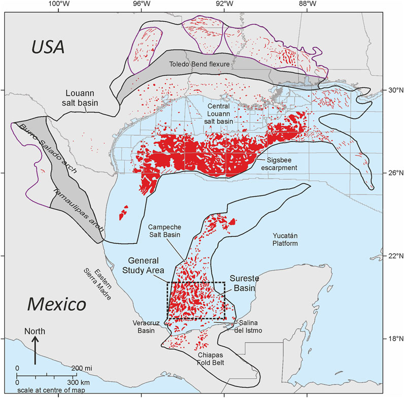
FIGURE 1. Outline of the Sureste Basin in Southern Mexico, the study area is located in the dashed box area in offshore section of the basin, we cannot reveal the exact location due to confidentiality agreements.
A complex geological history and the fact that exploration has only recently begun to focus on deep-water makes the Sureste Basin an ideal area to test the stratigraphic forward modelling program Onlapse-2D. Within the study area there is good quality seismic, however it lacks the vertical resolution to image detailed stratigraphic relationships. The overall tectonic history of the Sureste basin is well defined, but it is less so in the study area. Therefore, we believe that Onlapse-2D can be used to improve the understanding of sediment deposition and structural processes within the study area, thereby adding value to the exploration process by improving reservoir and seal predictions.
The structural history of the Sureste Basin, and indeed the whole of the Gulf of Mexico is the manifestation of complex plate tectonics resulting from the breakup of Pangea around 250–170 Ma. During the Middle Jurassic, counter-clockwise rotation of the Yucatan plate pulled the Sureste Basin away from the North American plate (Salvador 1987), (Hudec and Norton 2019), (Davison, et al., 2021).
Deposition of the Louann Salt occurred in the Bajocian (Middle Jurassic) (Pindell, et al., 2019) across stretched continental crust of the Gulf of Mexico. Oceanic spreading is believed to have begun soon after deposition of the Salt and continued until the end of the Berriasian (Early Cretaceous) (Stern and Dickinson 2010). This sea-floor spreading divided the Louann Salt into two segments with the salt provinces in the US Gulf of Mexico and Mexico’s Sureste Basin (Figure 1) (Hudec and Norton 2019).
After cessation of rifting in the Early Cretaceous, the Gulf of Mexico began to slowly subside owing to thermal cooling and sediment loading, producing a northwest-downward tilt to the Sureste Basin (Davison 2020) (Davison, et al., 2021). For the remainder of the Cretaceous, carbonate deposition dominated the basin with shelfal systems found around the south and eastern rim of the Basin, and fine grained carbonate clastic sediments deposited in the deep-water areas of the Sureste Basin (Padilla y Sanchez, 2007; Shann, et al., 2020).
The passive margin phase of basin infill in the Sureste Basin came to an end at the start of the Late Cretaceous with the start of the Mexican Orogeny. Cover shortening, in the form of folding and thrusting, propagated north-eastwards into the Sureste Basin (Shann, et al., 2020). Pre-orogenic salt diapirs were rejuvenated by squeezing, producing allochthonous salt sheets, which are most strongly developed in the onshore and shallow water zones (Davison 2020).
The drowning of the carbonate reefs in the Lower Palaeocene marks the end of carbonate dominance in the Sureste Basin and from this point onwards deep-water siliciclastic sedimentation dominated the basin, continuing until present day. However, carbonate sedimentation continued along the eastern rim of the basin along with isolated carbonate reef build ups (Davison, et al., 2021) (Shann, et al., 2020).
Thick Lower Miocene sands are evident across the offshore Sureste Basin and correspond to onshore formations (Shann, et al., 2020). The shelf margin in the Lower Miocene is located in the present day southern onshore region of the Sureste Basin. The shelf margin migrated northwards throughout the rest of the Miocene and until its present-day position in the offshore area of the Sureste basin (Gomez Cabrera and Jackson 2009). Throughout this time the main siliciclastic sediment input into the basin came from the southern part of the Eastern Sierra Madre and Chiapas area.
The Chiapanecan Orogeny began during the Miocene (18.0 Ma) (Davison, et al., 2021) and is responsible for a short lived but crucially important phase of compressional tectonics that affected the Sureste Basin. Between 13.8–11.6 Ma, this phase triggered allochthonous salt sheet development across the basin. The tectonic event produced what is known as the Chiapas Fold-and-Thrust Belt (Mandujano-Velazquez and Keppie 2009) and is associated with onshore volcanic activity (Stanbrook, et al., 2020). This event also produced intense deformation extending across a zone up to 600 km North from the southern margin of the Sureste Basin (Davison, et al., 2021) (Shann, et al., 2020) (Davison 2020). The culmination of this tectonic event is a regional strong erosional unconformity.
This Middle Miocene event effectively subdivides the stratigraphy into three; (i) a pre-orogenic, Oligocene – Lower Miocene section, which was folded prior to emplacement of the extensive salt canopy; (ii) a syn-orogenic Middle Miocene deep-water turbidite system that is associated with the emplacement of an extensive salt canopy; (iii) a post-orogenic infill, of Late Miocene to Pliocene age, which is not affected by the Chiapaneco folding (Shann, et al., 2020).
Within the study area (Figure 2A) Sand Injectites are observed to penetrate from Middle Miocene stratigraphy through the lower section of the Late Miocene, and cease being observed in the later stages of the Tortonian (Late Miocene). In the later stages of the Tortonian pockmarks are observed to occur above where the injectites are observed (Figure 2B). While the existence of sand injectites in other basins (e.g. North Sea, Onshore California) is well documented, and oil saturated sandstone intrusions have been recognized in some Gulf of Mexico core (Andrew Hurst, pers. comm. 2021) we are unaware of any published documentation of their presence in the southern Gulf of Mexico, including the offshore Sureste Basin.
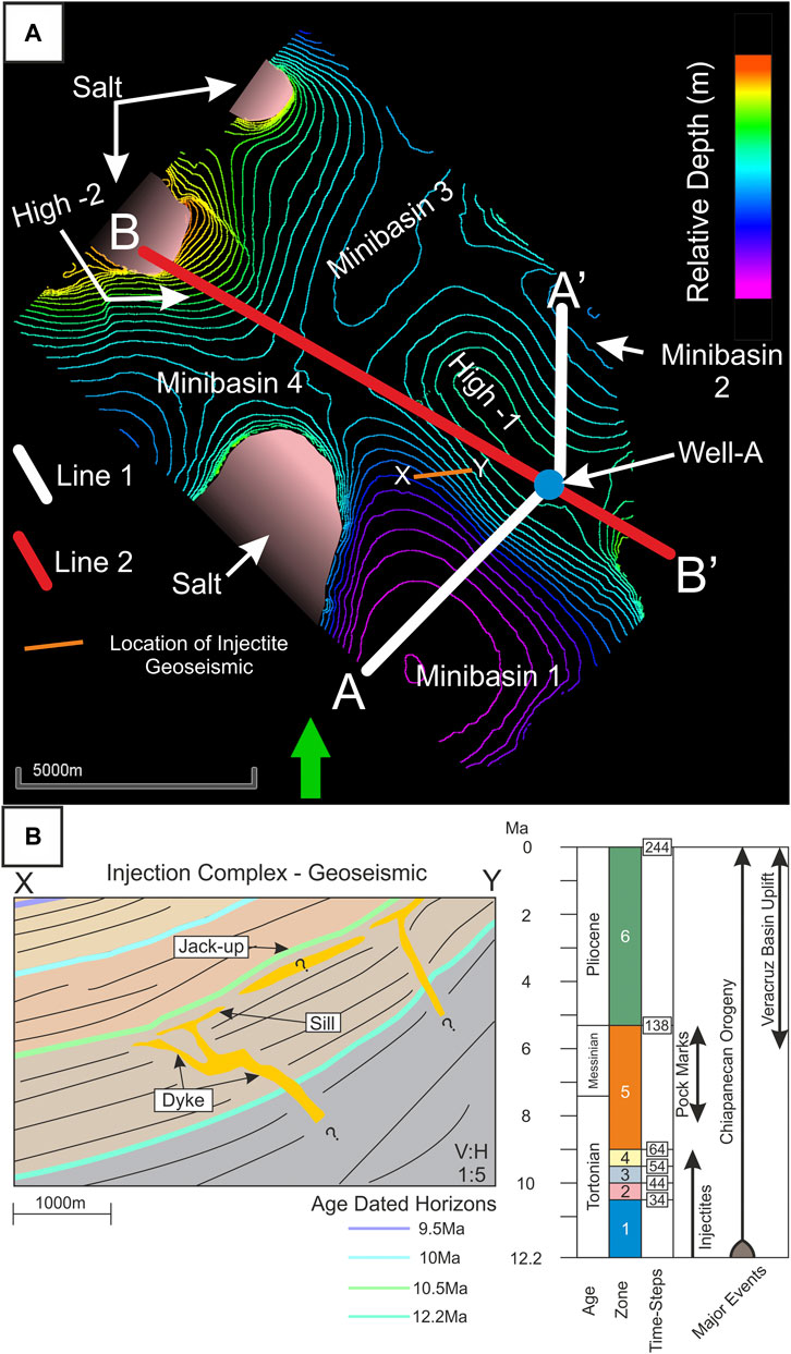
FIGURE 2. (A) Location of Well-A superimposed over a relative depth map of the 12.2 Ma horizon interpretation, and the two modelled cross-sections Line 1 and Line 2. Frame of reference has been rotated to preserve confidentiality. (B) Geoseismic section X-Y, located to the southwest of High-1, showing a sand injectite dyke and sill complex within Lower Tortonian section. The interpreted timing of sand injection shown on the stratigraphic chart is based on observed sediment response to local sea floor uplift (jack-up above injectite sills). Pockmarks in the overlying Upper Tortonian to Messinian section indicate a second pulse of fluid-flow.
After the development of the Mid-Miocene Chiapas Fold-and-Thrust belt due to the Chiapaneco Orogeny the tectonic development of the Sureste Basin was dominated by two events. The first was a long lived gradual downslope gravity collapse over the shelf-slope sediments into the Gulf of Mexico. This divides offshore Sureste Basin into three regions; an updip set of extensional salt withdrawal minibasins, a mid-slope translational area with widespread partly amalgamated salt canopy, and a lower-slope set of large compressional anticlinal folds (Shann, et al., 2020). The second late compressional event effects the south-eastern part of the Sureste basin, uplifting the entire Veracruz basin to the west of the Sureste Basin caused by Pliocene volcanic episodes (Padilla y Sanchez 2007).
The overall aim of this study was to utilize a forward stratigraphic modelling software, Onlapse-2D to better understand the tectonostratigraphic evolution of the Late Miocene section in three adjacent minibasins in a geologically complex area located in the offshore Sureste Basin. The secondary objective was to validate and develop the capability of Onlapse-2D. We present here the results of two modelled cross-sections, and will demonstrate how the modelling of two cross sections allowed us to better understand the spatiotemporal evolution of structural growth and how sediment input may have evolved through time. We will also demonstrate how analyzing discrepancies between the model out and subsurface data can be a vital source of information. In the process, we exhibit how Onlapse-2D enables the user to determine the likelihood of reservoir and seal present in a given stratigraphic interval.
For this project, we utilized a subset of a 3D Kirchhoff Pre Stack Depth Migrated seismic. The seismic data provided good image quality allowing for the mapping of structural and stratigraphic surfaces but did not provide direct imaging of reservoir systems. Structural and seismic surface interpretations were tied to and dated by biostratigraphic data in Well-A. We were provided access to full well log data that included, Gamma Ray, Resistivity, Neutron Porosity, Density, VShale, and Image Logs interpretations.
Stratigraphic Forward Modelling is the use of mathematical formulae and algorithms to create synthetic stratigraphy, with the aim of understanding and predicting dynamic sedimentary systems (Burgess 2012) (Huang, et al., 2015). Natural systems are complex and dynamic, and consequently are difficult to model. Stratigraphic Forward Modelling can be broadly split into two end member methods, Process Based Modelling and Geometric Modelling, each with its own advantages and disadvantages (Paola 2000; Burgess 2012; Huang, et al., 2015).
Process based modelling is built on the concept of numerically modelling the physics of sediment transport through methods such as sediment diffusion (e.g. (Rivenaes 1992), (Granjeon 2014)) or the Navier-Stokes equation; for example (Griffiths, et al., 2001; Basani, et al., 2014).
Geometric models do not consider the dynamics of sediment transport. Instead they use a simple set of rules to model the overall thickness and stratal geometry of discrete stratigraphic intervals rather than the individual depositional events within the intervals; for example (Sylvester, et al., 2015).
Previous simulations of structurally active mini-basins typically use two approaches; Generic models using simple rules for sediment deposition in idealized mini-basin geometries (e.g. Sylvester et al., 2015). These are rapidly generated, and give useful insights into the general processes of mini-basin evolution, but they typically do not replicate real world examples. Models that apply more complex algorithms to simulate the flow of individual turbidity currents, stacking these to build up a synthetic stratigraphy (e.g. Burgess, et al., 2019).
In this paper we use a different approach with Onlapse-2D. Our fast computational model uses simple rules to match the seismic and well data in a real world example, iterating towards a best-fit solution through hundreds of simulation runs.
Onlapse-2D is a stratigraphic forward modelling program, developed in Matlab that simulates the tectonostratigraphic evolution and development of structurally controlled, deep-water minibasins. It uses four inputs; Initial Basin Structure, Background Sedimentation Rate, Structural Growth Profile and Rise, and a variable rate of rise of a Clastic Limiting Surface. The Clastic Limiting Surface is a horizontal like used to determine whether new gravity flow sediment is deposited at a given position on the cross-section. Onlapse-2D combines these inputs using simple rules to generate realistic looking basin architectures. Onlapse-2D simulates the simultaneous growth of structures and a variable rate of sediment deposition. Both rates may be derived from real data (as in this paper) to simulate structural and stratigraphic evolution of a real world basin. Onlapse-2D is also used to simulate idealized basins to explore how the interaction between structural growth and deposition generates different stratigraphic architecture (Christie 2021).
To achieve the stated aims in the introduction we selected an area with good quality, high resolution seismic data and well control (good age dating) in a region with 3-dimentional structural complexity. We constructed and modelled two cross sections. The first traverses Minibasin-1 passing through Well-A and into the adjacent Minibasin-2. The second cross-section, Line 2 intersects Line 1 at Well-A, traversing Minibasin-2 and Minibasin-4.
This study was conducted in the offshore area of the southern Sureste Basin in Mexico (Figure 1). In all other maps and sections presented here cardinal points have been rotated to preserve confidentiality but we use a consistent reference direction in all figures. Two 2D intersecting cross sections were modelled, with these locations chosen to investigate different phases and different styles of deformation in different orientations. There are four minibasins within the study area which extend beyond the boundaries of the study area. The center-piece of the study area is a North-West to South-East trending long lived structural high known as High-1. Minibasin-1 is to the South-West of this high and is flanked to the North-West by the largest of the salt cored highs; at its longest and widest extent, it is 5 km by 5 km. Minibasin-2 is located off the Northern flank of High-1 and measures 4 km in length and 2 km in width. To the North of High-1 and Minibasin-2 is Minibasin-3 measuring 5 km by 6 km and is flanked to the North and West by two salt cored highs. Minibasin-4 is located off the North-West of High-1 and at its widest extent and at its maximum length is 3.5 km (Figure 2A). The main deep-water depositional systems of interest entered at the south of the basin in Minibasin-1 and 2, flowing axial to the long lived central high into Minibasins 3 and 4.
The boundary conditions for Lines 1 and 2 are as follows;
- Total Simulation Time: 12.2Mya (from Middle Miocene until present day)
- Time per Time-Step: 50ky
- Total number of Time-Steps: 244
- Basin Length:
o Line 1: 8,550 m
o Line 2: 10,875 m
- Horizontal Resolution: 25 m.
Line 1 and 2 modelled a total time interval of 12.2 Ma, but focused on the period 12.2– 5.3 Ma (Mid-Miocene to Late Miocene). After 5.3 Ma, the modelling was completed to a lower spatial resolution. The time interval of 12.2 Ma is split into six zones that correspond to different Time-Steps.
- Zone 1: Time-Step 1–34 (12.2–10.5 Ma)
- Zone 2: Time-Step 35–44 (10.45–10 Ma)
- Zone 3: Time-Step 45–54 (9.95–9.5 Ma)
- Zone 4: Time-Step 55–64 (9.45–9 Ma)
- Zone 5: Time-Step 65–138 (8.95–5.3 Ma)
- Zone 6: Time-Step 139–244 (5.15–0 Ma)
The four main inputs to the model and described below.
The initial basin structure (Figure 3A) represents the basin floor bathymetry at the start of the model (Time-Step 0). The starting point for constructing this is to use the isopach of the interval beneath the deepest interpreted seismic horizon that onlaps onto the strong Middle Miocene unconformity as a guide (Figure 3E). Beyond the depositional edge of that deepest interpreted horizon, the isopach is not defined, and therefore the Initial Basin Structure is derived by a process of iteration.
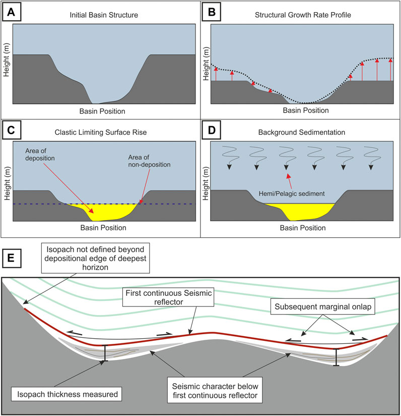
FIGURE 3. (A) The Initial Basin Structure at Time-Step 0, Figure 4 illustrates how we derive this from seismic data. (B) Dotted line represents the Structural Growth Profile, with red arrows indicating the rate of rise being applied to the Basin Structure (dark grey structure). The Structural Growth Rate Profile consist of multiple profiles, in this example it is a single profile. (C) Blue dotted line is the Clastic Limiting Surface, if there is available accommodation space below then gravity flow deposit packages are deposited, if not then no deposition occurs. (D) A uniform thickness of background sediment is deposited along the cross-section, through pelagic and hemi-pelagic settling. (E) The Initial Basin Structure at Time-Step 0 is derived by mapping the first continuous seismic reflector (red) and measuring the thickness of the isopach below it. Inspection of the subsequent and underlying, strata to identify patterns of onlap and geometry allow us to infer how much topography existed at Time-Step 0 and how much topography may have been created by subsequent structure growth.
The Structural Growth Profile is a curve that defines the shape of the growing structure, this curve varies through space, but remains constant through time. The Structural Growth Rate is a user defined curve that defines the amount of growth applied to the Structural Growth Profile through time. This is spatially uniform, but varies through time. Combining the Structural Growth Profile and the Structural Growth Rate gives the Rate of Rise of the Structural Growth Profile (Figure 3B). This is the amount of rise in mm/yr converted to m/Time-Step that is applied to the basin structure through vertical shear.
The first iteration is determined through taking the Initial Basin Structure and measuring its height from the lowest point in the basin. We then compare each point along the cross-section to its height at the present day from the lowest point in the model, which gives us a simple way of calculating the average growth in mm/yr along the cross-section. This provides us a basic Structural Growth Profile, which is refined iteratively during the modelling process to match a predetermined set of criteria. For this study, two basic criteria were applied to the Structural Growth Profile. The first is that it must replicate the form of the final structure visually, and the second is that it must do so to a tolerance of ±25 m. Onlapse-2D can model complex structural scenarios in which multiple structural processes act in the same place by combining several Structural Growth Profiles to represent different components of the structural development (salt diapirism, fold growth etc.).
The Rate of Rise of the Clastic Limiting Surface is the amount of rise in mm/yr converted to m/Time-Step that is applied to the Clastic Limiting Surface (Figure 3C). The Clastic Limiting Surface is used to determine whether new gravity flow sediment is deposited at a given position on the cross-section. The Clastic Limiting Surface is a line that delineates above which, no sediment gravity flow deposits are preserved, and below which if there is accommodation, they are preserved and are given the name Gravity Flow Deposit Packages. This is a user-defined horizontal level that can rise or fall with time. The Clastic Limiting Surface provides a straightforward means of determining the amount of sediment being captured by a basin over time. While in nature, the amount of sediment input into a minibasin can be controlled by a variety of external geological processes (e.g. relative sea-level fall, climate, up-dip avulsion of sediment feeder channels etc.), these factors are rarely well understood and cannot be quantified. Onlapse-2D does not require knowledge of larger scale variables or inputs. The user makes no assumptions and instead controls only the amount of sediment captured within the minibasin at any one time, using the Clastic Limiting Surface. The Clastic Limiting Surface is not necessarily equivalent to a base-level, equilibrium surface, or even a spill point (because the user may not know that level for the basin on the chosen line of section). The Rate of Rise of the Clastic Limiting Surface is determined by local seismic and well data only (e.g. reflection seismic and well data, especially biostratigraphic data that contains information on the rate of sediment accumulation in the basin through time). It is a user-defined surface that is specific to that minibasin. It does not require knowledge of larger scale variables, nor does it require the user to know where the basin was relative to the sediment fairway, or whether the minibasin was close to the regional slope gradient, or structurally perched above the regional slope.
In this example, the initial rate of rise applied to the Clastic Limiting Surface were based on the calculated average sedimentation rates from Gomez Cabrera & Jackson (2009), which are not corrected for compaction so are likely to be an underestimate. Starting at the lowest zone, we worked progressivly up through the stratigraphy, making adjustments to the Rate of Rise of the Clastic Limiting Surface so that the stratal patterns (onlap and offlap) and thickness within the zone match the subsurface data. The tolerance for thickness match is ±25 m.
This is the amount of sediment deposited uniformly along the cross section through pelagic and hemipelagic settling (Figure 3D). While it is spatially constant at any one time, the rate of Background Sedimentation can change through time. We calculated this from two interpreted condensed sections within the interval of study in Well-A that had good biostratigraphic age constraint. The deeper, oldest condensed section included an average background sedimentation rate of 0.022 mm/yr, and the second condensed, younger section averaged 0.047 mm/yr.
Several assumptions are made during the processes of producing models with Onlapse-2D. Within the model we assume that deposition only comes from sediment gravity flows and background sediment, and that there is no significant contributions from other processes such as carbonate build-ups. Onlapse-2D is unable to model erosion, and also assumes that all gravity flow deposit packages are horizontal at the time of deposition, which means that Onlapse-2D can’t directly model positive depositional topography or depositional erosive features such as channel scours. Onlapse-2D also assumes that all structural movement occurs through vertical shear, and that there are no major horizontal components to structural movement. Onlapse-2D also inherits all the assumptions that are made when matching to subsurface data such as reflection seismic or well logs.
Compaction is not currently included within the model; therefore, estimates on the Background Sedimentation Rate and depositional rates of the Gravity Flow Deposit Packages are an underestimate. In this example this does not invalidate the model because we are able to obtain realistic simulations of the real world geometries indicating differential compaction is not a significant factor in this basin.
Geoscientists commonly associate yellow coloured layers with sandy lithologies. Onlapse-2D does not assign a lithology to the modelled Gravity Flow Deposit Package, only stating that the rise of the Clastic Limiting Surface is generated by sediments deposited through gravity flow processes. The Gravity Flow Deposit Package represents any package of flow deposits, including low and high-density turbidites, calci-turbidites, and mass transport deposits. The interpreting geoscientist must, through their geological understanding (e.g regional knowledge, seismic or well data, geological models) make an informed decision on what type of gravity flow deposit is represented in any given part of the active depositional package.
The procedure for generating stratigraphy using Onlapse-2D is to: 1) generate an Initial Basin Structure; then for each Time-Step of the model: 2) apply the Structural Growth Profile rise for that Time-Step; 3) apply a rise to the Clastic Limiting Surface; if there is accommodation, then a gravity flow deposit package is deposited up to the Clastic Limiting Surface for each Time-Step 4) drape a uniform thickness of background sediment across the cross-section (Figure 4). Steps 2–4 steps are repeated until the correct number of Time-Steps is completed.
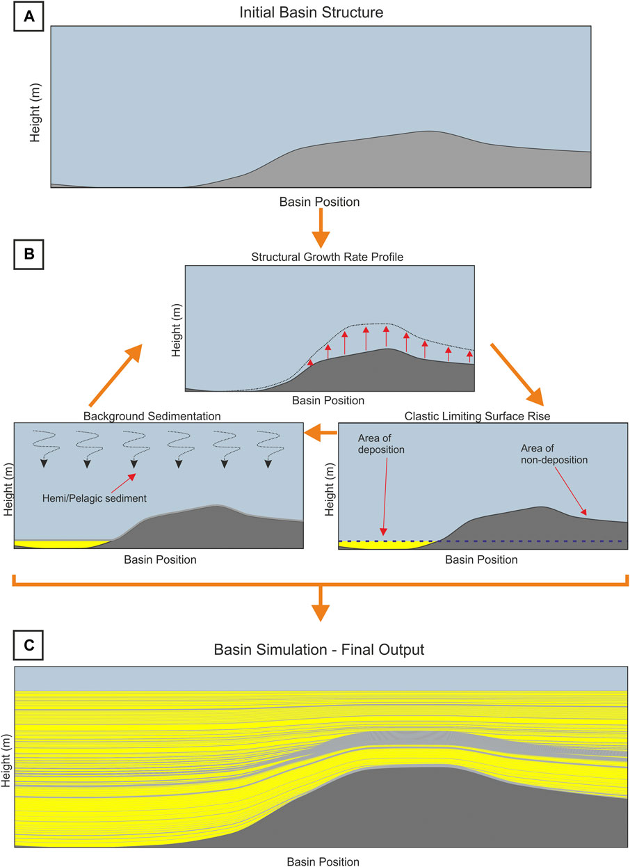
FIGURE 4. (A): Time Step 0 shows the Initial Basin Structure with height in meters on the Y axis and Basin Position on the X axis. (B): Onlapse–2D applies a structural growth rate to the initial basin structure, then Onlapse–2D applies a rise to the clastic limiting surface and if there is accommodation available gravity flow deposit packages are preserved. After this, Onlapse–2D applies a uniform thickness of pelagic/hemipelagic sediment across the cross section. Section B is repeated a number of times as dictated by the number of Time-Steps. Producing a final cross section, (C).
After each iteration of the simulation, we compared the generated stratigraphy to the subsurface data consider if the stratigraphy generated is consistent with the subsurface data and what, if any, differences can be found. First we measure the thickness of modelled intervals at key points along the cross-section. Key points are equally spaced points along the cross-section, for example every 1,000 m, but also include important features of interest such as the tops of anticlines, the deepest points of synclines, or wells. This is compared to the same interval isopachs on the seismic section that is the basis for the modelled 2D profile. Second, we inspect the match between the stratal relationships generated in the model and those observed on the seismic line; for example, where there are onlaps on the seismic line, there should be onlaps on the model. Third, we consider the seismic facies of each zone, and the lithology. While Onlapse-2D does not explicitly define the lithology, the seismic facies, or mappable architectural elements within an interval, are good indicators of the type of gravity flow deposits and a proxy for the relatively speed at which the package was deposited. Intervals with active siliciclastic systems should match the zones in the Onlapse-2D model with high values for the Clastic Limiting Surface (more deposition per unit time). Spikes in the rate of Clastic Limiting Surface rise (i.e. zones deposited at the fastest rate) commonly correspond on seismic data to distinctive thick laterally extensive discontinuous, chaotic seismic facies interpreted as probable mass transport complexes, however they can also represent a mega-turbidite deposit.
If a good match is not achieved, then the input variables (e.g. Clastic Limiting Surface, Structural Growth Profile, and Initial Basin Structure) are altered until the modelled stratigraphy fits within an acceptable range. For example, alteration of the input variables can include increasing or decreasing the rates of rise of the Clastic Limiting Surface or the Structural Growth Profile, adding additional Structural Growth Profiles, changing the shape of the Initial Basin Structure. For this study the iteration process continued until the generated stratigraphy matched the subsurface data. If the changes do not iterate towards a good fit to the subsurface data, there are two principal reasons. The first is that the structural simulation may not include all the structural processes within the basin (e.g. salt withdrawal) in some cases the difference may be resolved by adding additional structural growth profiles that represent some of the missing processes. The second is that the discrepancy may be caused by a depositional process that cannot yet be modelled through the Onlapse-2D method (e.g. erosional or constructional depositional topography).
We found that the modelled outputs of the final basin structure, thicknesses of modelled zones, and lateral extent of Gravity Flow Deposit packages found within them was a good fit to seismic and well data (Figure 5). A single, simple Structural Growth Profile that grew at a constant rate at each Time-Step was used. The Background Sedimentation Rate, derived from well based condensed section information increased in increments through time. The rate of rise of the Clastic Limiting Surface was more varied in both magnitude of rise per Time-Step and the duration of each rise (Figure 6). The combination in Figure 6 is non-unique but provided us with the closest fit to the seismic and well data of multiple model runs.
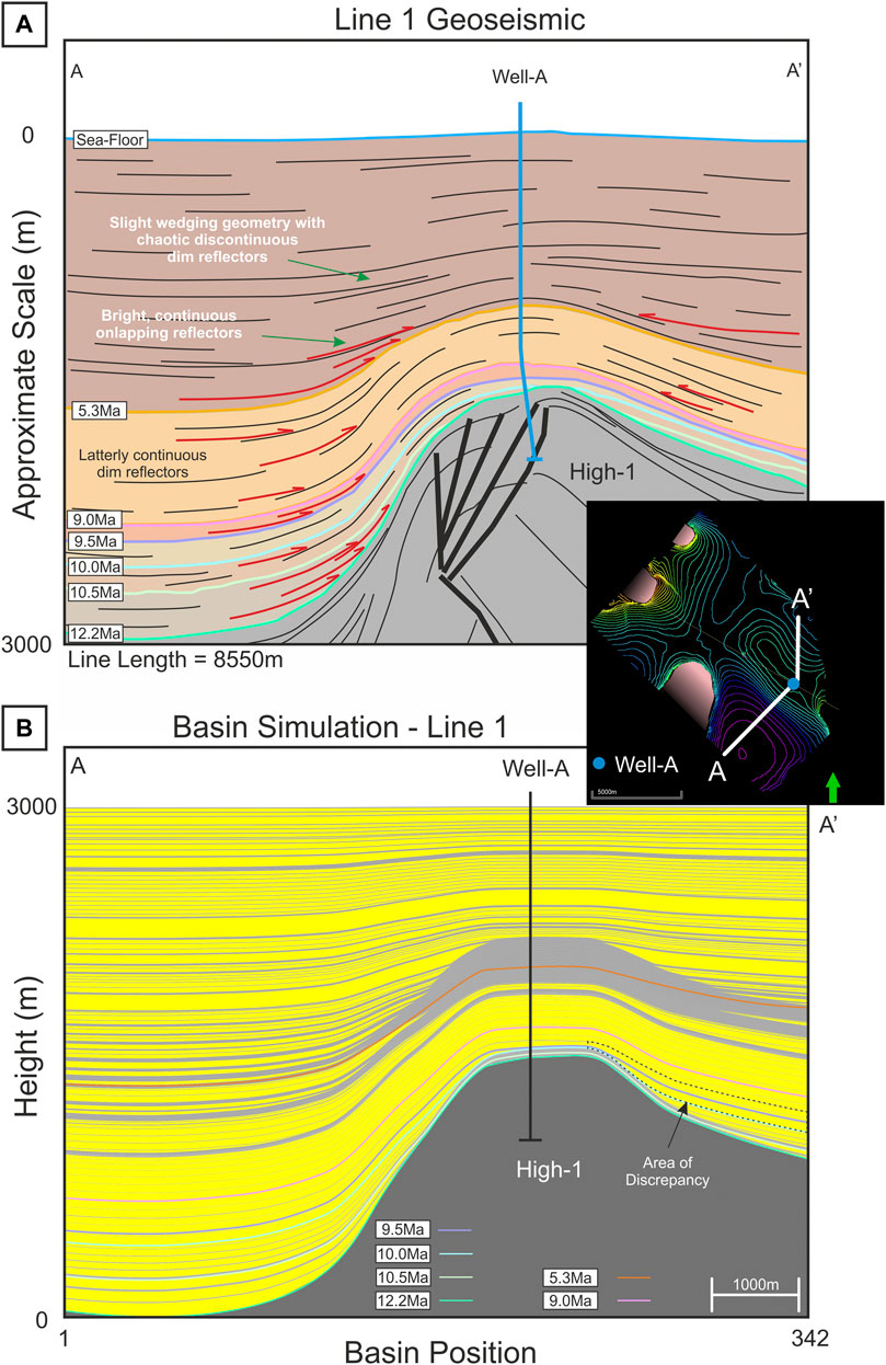
FIGURE 5. (A) Geoseismic cross-section of Line 1 showing the position of Well-A, age-date horizons tied to Well-A, and brief annotations of the seismic character. The red arrows show some of the major onlapping reflectors and thick black lines represent faults in High-1. Modelling was completed from 12.2 Ma until present day. With 12.2–5.3 Ma being the focus and matched quantitatively to the subsurface data, while 5.3 Ma until present day was modelled to a lower, qualitative resolution only. (B) Onlapse-2D final simulation output of Line 1. We found there to be an overall good fit between this and the subsurface data shown in (A). The model produces good fits with the overall basin structure and form, as well as the thicknesses and stratal geometries found within the interpreted horizons. An area of discrepancy is shown on the northern flank of High-1.
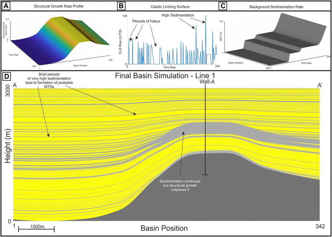
FIGURE 6. Inputs used to model the evolution of Line 1. (A) 3D Representation of the Structural Growth Profile, X axis represents position in space, Y Axis represents position in Time, Z axis represents the growth that the structure grows in meters per time step. (B) The rate of rise of the clastic limiting surface; showing the sporadic nature and short lived time in which sediment gravity flows occur in the cross-section. (C) Background Sedimentation Rate; derived from data from Well-A. X Axis represents position in space along the cross section, Y axis represents position in time, and Z axis represents amount of background sediment deposited in meters. (D) Final simulation for Line 1, highlighting periods of very high, but short lived, sedimentation (which probably correspond to MTDs) and periods of hiatus in sedimentation.
Within Time-Step 45–54 (Zone 3) and Time-Step 55–64 (Zone 4) we found that on the northern flank of the High-1 there was a localized but significant mismatch between what the seismic data indicates, and what the Onlapse-2D model predicted to be deposited. We found there was an increasing amount of over thickening into the northern section of the basin. The implications of this discrepancy, and how we corrected for it will be discussed further in the discussion section.
As with Line 1, we found that overall the modelled basin structure, thickness of the zones within the interval of interest, as well as the lateral extent of the Gravity Flow Deposit Packages within those zones were a good fit to both the seismic and well data (Figure 7). All boundary conditions were consistent with Line 1, except the Basin Length which was 10875 m. The area above the section of interest in Line 2 could not be modelled with a single, simple Structural Growth Profile (Figure 8A). To fit the stratigraphy above the section of interest, we required two different components of the Structural Growth Profile with different growth histories. The first component of the Structural Growth Profile was consistent with compressional folding, similar to Line 1, but with two discrete phases. The second component of the Structural Growth Profile was a longer time wavelength and was required to account for the significant structural high at the NW end of Minibasin-4, and is consistent with salt withdrawal and diapirism. The timing of the interactions of the two Structural Growth Profiles is consistent with regional knowledge, and the spatial distribution is consistent with regional knowledge and structural geological principles (Padilla y Sanchez 2007) (Padilla y Sanchez 2014) (Davison 2020). We will expand on this in the discussion. As stratal patterns are generated in Onlapse-2D through the interaction between Structural Growth and the rise of the Clastic Limiting Surface, changes to the Structural Growth Profile meant that we needed to create a new rate of rise of the Clastic Limiting Surface. Changes to the Rate of Rise of the Clastic Limiting Surface were focused on the interval of interest (12.2–5.3 Ma), and included increasing and decreasing the rise of the Clastic Limiting Surface in M/Time-Step, changing the Time-steps in which the rise occurred, and the addition of a continuous rate of rise between 7.8–5.3 Ma. However, the Background Sedimentation Rate remains the same (Figure 8C).
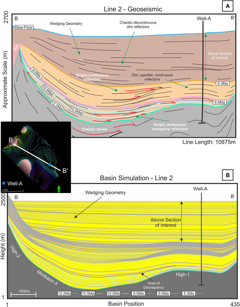
FIGURE 7. (A) Geoseismic cross-section of Line 2. Line 2 crosses both High-1 and High-2, with High-2 containing salt. The wedging geometry seen in geoseismic cross-section is above our area of interest, but is still modelled at a lower resolution. (B) Onlapse-2D final simulation, overall within the section of interest there is a good match between model and the geoseismic. The model is able to match the general form of the basin as well, and major onlapping reflectors seen in 8a, occur in the modelled simulation. An area of discrepancy is highlighted within MiniBasin 4.
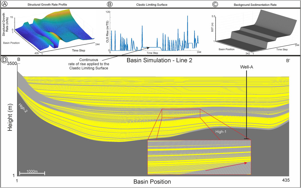
FIGURE 8. Inputs used to model the evolution of Line 2. (A) 3D representation of the Structural Growth Profile, a much more complicated structural growth history is visible compared to Line 1. A combination of 2 Structural Growth Profiles, one represents the effects of salt tectonics and the other representing the growth of the Fold. (B) The rate of rise of the Clastic Limiting Surface shows a more sustained input of gravity driven currents to achieve a good match compared to the more sporadic input in Line 1. (C) Background Sedimentation Rate used in Line 1 is used in Line 2. (D) Final simulation for Line 2. Insert section highlights thin gravity flow deposits, with red arrow showing the direction of onlap onto the basin flank.
Within Zone 4 (Time-Step 55–64) of Line 2 we found a localized but significant discrepancy between the final best fit simulation and the subsurface data. This mismatch could not be eliminated by simple adjustment of inputs. This discrepancy, which was focused around Well-A, is highly informative, providing additional information about the evolution of the section. If the simulation matched the thicknesses found within Well-A, we found that there would be significant (up to 125 m) of extra siliciclastic sediment deposited within the mini-basin to the north-west. The implications of this informative discrepancy, as well as how we corrected the simulation are considered in the discussion.
We deliberately kept the Structural Growth Profile and its rate of rise as simple, consistent, and geologically plausible as possible in order to make comparisons between iterations easier. In the model runs of Line 1, we found keeping a single, simple Structural Growth Profile that grew at a constant rate of rise per Time-Step produced the best fit model for our subsurface data. However, we subsequently determined that the Structural Growth History for this study area is more complex than we initially supposed. As we will discuss, there are two phases of structural movement in the study area, but due to the orientation of Line 1, it did not show evidence of this. This illustrates the importance of using multiple lines of section when modelling in 2D.
For Line 2 we applied the same principle, starting with a single, simple Structural Growth Profile that grew at a constant rate of rise per time-step. The rate of rise of the Clastic Limiting Surface used for Line 1 was also used for Line 2. The rationale being that, if the modelling for Line 1 was the correct solution for Well-A, High-1 and surrounding minibasins, we would be able to produce a close fit to the seismic and well data for Line 2. We would expect minor adjustments to either the rate of rise of the Clastic Limiting Surface or the Structural Growth Profile to occur simply because of the 3D nature basin evolution. However, using a simple, single Structural Growth Profile and the rate of rise of the Clastic Limiting Surface from Line 1 did not provide a good match in Line 2 for the seismic or well data. Minor iterative changes to the rate of rise of the Clastic Limiting Surface (changing the magnitude of rise or Time-Steps of the rise), the Structural Growth Profile, or the Initial Basin Structure could not overcome the differences in the model and the subsurface data.
Instead, major changes to the Structural Growth Profile were needed to get a close match to the subsurface data. The first major change was to significantly change the Structural Growth Profile (Figure 9), both temporally and spatially. The first profile consisted of two phases of folding, focused on High-1 and around Well-A, phase one occurs between Time-Step 0–65 (12.2–8.95 Ma) with maximum fold growth occurring between Time-Steps 50–59 (9.7–9.45 Ma). Phase two of this folding occurs between Time-Steps 80–244 (8.2–0 Ma), with the maximum fold growth occurring at Time-Step 88 (7.8 Ma). The timing of these folding phases indicates that they are likely to be related to the Chiapanecan Orogeny (18–0 Ma) (Padilla y Sanchez 2007) (Mandujano-Velazquez and Keppie 2009) (Padilla y Sanchez 2014) (Davison, Pindell and Hull 2021).The second profile included the growth of a salt diapir at the north western end of Line 2, and that replicated the wedging geometry we observed in Line 2, with the stratigraphy thinning north-westwards onto the salt cored high (Figure 9). Regional studies confirm that salt movement has continued in the Sureste Basin (Padilla y Sanchez 2007) (Gomez Cabrera and Jackson 2009) (Ruiz-Osorio, 2018) (Davison 2020). Having three distinct phases of structural growth on Line 2 allowed us to have a much closer match to both the subsurface data. The last phase of structural growth had the greatest impact on the high at the northern end of Line 2, and that high is known to be a salt diapir (Figure 9).
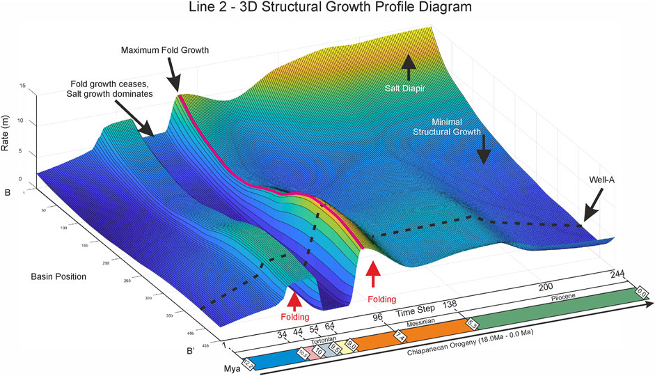
FIGURE 9. 3D representation of the rate of rise of the Structural Growth Profile through time. X–axis represents position in time, Y–axis represents basin position along Line 2, Z–axis showing the rate of rise in meters per Time-Step. Diagram shows the combination of two Structural Growth Profiles through time. Profile 1 was consistent with compressional folding over High-1, Profile 2 is focused on salt diapirism and withdrawal at High-2. Fold growth (Profile-1) dominates in two distinct phases, phase one occurs from 12.2 Ma until ceasing at 9.0 Ma, at this point Profile 2 (salt growth) dominates until 7.8 Ma, at which point compressional folding begins again. Profile 1 continues to dominate until the middle Pliocene when fold growth tapers off. At this point, salt tectonics dominates, represented by Profile 2.
So how can we have two lines that intersect that have apparently such different structural histories? We believe this is because both salt withdrawal and compressional folding are highly three dimensional in this basin. There are three distinct phases of structural activity represented on line 2, with two distinct structural processes active within the study area: salt diapirism and withdrawal, plus two distinct phases of folding which occurred between 12.2–8.95 Ma and between 8.2–0 Ma.
Why did we not see the two phases of folding in the model for Line 1? A line of section that is parallel to the fold axis of an episode of folding (i.e. strike to the shortening direction) will not show any sign of the existence of that fold episode. That folding episode may uniformly raise or lower the line across its whole length, and we may not see differential uplift/subsidence in that direction. Conversely, a line that is at an oblique angle to a fold axis should show obvious evidence of that episode of folding.
In the study area we have 2 phases of folding whose orientations are nearly orthogonal (Figure 10). In the frame of reference used in this paper Phase 1 produces dominantly north-south fold axes, Phase 2 creates southwest-northeast fold axes. Line 1 is at a high angle to phase 1 and therefore shows phase 1 folding, but it does not cross any phase 2 structures. Conversely, line 2 intersects both structures of phase 1 and 2. For this reason line 1 can be modelled without requirement for phase 2 structuring as part of the model. Line 2, however, requires incorporation of both phase 1 and 2 of folding.
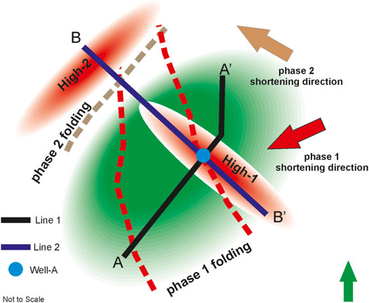
FIGURE 10. Schematic drawing of the structural components of study area. Red dotted line represents phase 1(12.2–8.95 Ma) fold axes that trend roughly North–South. Brown dotted line represents the phase-2 (8.2–0.0 Ma) folding axes which trends southwest-northeast. Phase 1 shortening direction is towards the southwest, phase 2 shortening direction is northwest. Line 1 does not intersect the fold axis of phase 2 folding, while Line 2 intersects both phase 1 and 2. Green area represents the minibasins found within the study area.
Likewise, we did not identify a separate signature for salt withdrawal in Line 1 because we believe the local salt is withdrawing predominantly in a north-south direction to produce the High-2 diapir at the north end of line 2. For this reason, line 2 needed to incorporate salt withdrawal and diapirism. Regionally, movement of salt found in the Sureste basin has continued until the present day, moving in a general northward direction (Gomez Cabrera and Jackson 2009) (Davison 2020).
Each component of the Structural Growth Profile reflects different structural controls on the basin, and show the amount of control that is exerted on the growth of structural accommodation through time (Figure 9). This is in agreement with regional studies that show the Sureste Basin is a tectonically active with compressional tectonics from the Chiapanean Orogeny (Padilla y Sanchez 2007) (Gomez Cabrera and Jackson 2009) (Padilla y Sanchez 2014) (Davison, et al., 2021) salt tectonics playing important roles the development of the region (Gómez-Cabrera and Jackson 2009) (Ruiz-Osorio, 2018) (Davison 2020). There are two distinct phases in the structural evolution of the cross-section where fold growth is dominant. Between these two phases, fold growth dramatically reduces from around 9.0–8.2 Ma, before increasing rapidly, peaking at around 7.8 Ma then decreasing over the course of the Pliocene (Figure 9). The timing of the first phase of folding appears to directly correlate to a major regional event, which is the development of the Chiapas Fold-and-Thrust Belt (13.8–11.6 Ma) and the associated intense deformation in the offshore Sureste Basin (Mandujano-Velazquez and Keppie 2009) (Davison 2020). However, the results from our modelling indicates that local tectonic movement continued post 11.6 Ma, and may be also related to the ongoing Chiapanecan Orogeny. Salt tectonics dominates in the Pliocene, and this is what forms the wedge-shaped stratal geometry seen in the area above the Miocene section of interest in Zone 6.
Figure 11 is a tectono-chronostratigraphic chart we extracted from the Onlapse-2D model of Line 2, with the timing and relative importance and contribution of the two structural processes shown in red and green to the overall structural movement of Line 2. Salt tectonics exerts continual influence on the structural evolution of the cross-section throughout time, with increasing influence and becoming dominant in the Pliocene. While the fold growth of High-1, is a more variable event through time, it is dominant in the Late-Miocene before and decreases through the Pliocene.
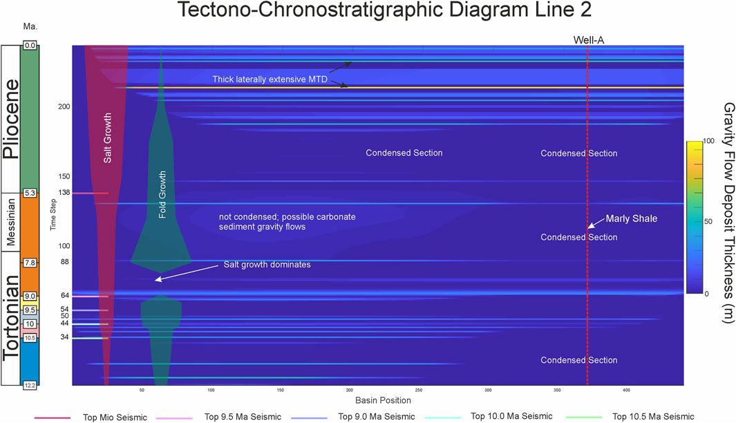
FIGURE 11. Tectono-Chronostratigraphic chart of Line 2, highlighting the temporal and spatial distribution of gravity flow deposits as well as their thicknesses. Superimposed onto the chart are representations of the two structural growth profiles used in modelling Line 2. The width of these profiles represents the relative strength that each profile exerts of the overall structural growth of Line 2. Salt Growth (Profile 2) is continuous through time, while Fold Growth (Profile 1) has two distinct phases, and can be seen to decrease rapidly in the Pliocene. Well-A shows multiple condensed sections in which no gravity flow deposits are intercepted. Section labelled “not condensed” is where Onlapse-2D had to introduce a small but continuous rise to the Clastic Limiting Surface, this deposited thin gravity flow deposits that onlap onto flanks of High-1.
The observation of sand injectites around the High-1 in the study area provides important independent evidence of two discrete phases of folding in the Onlapse-2D model output (Figure 2). Sand injectites are observed to penetrate from the Middle Miocene through the lower section of the Late Miocene, and are not active in the Late Tortonian. The remobilization of sands occurs when fluid overpressure forcefully injects poorly consolidated sand into the host strata (Vigorito and Hurst 2010) there are many ways in which fluid overpressure can occur; for example depositional compaction or fluid volume change. As shown by Palladino et al. (2016) contractional tectonics, such as we see here, also increases the pore-fluid pressure and can result in sand injectites. The remobilization of sand occurs throughout first phase of compression that is modelled in Onlapse-2D and, crucially, injectites are observed to terminate close to the time when the first phase of compression ceased in the model (Time-Step 65). No injectites are observed in the later stages of the Tortonian. Pockmarks, which are evidence of over-pressured fluid escape (Chand, et al., 2017) are observed to occur around the time that the second phase of contraction occurs (Time-Step 80); indicating that while vertical migration of fluids continued and may be related to local compressional tectonics, the remobilization of sand ceased when the over-pressured fluids vented to the surface.
To date Onlapse-2D has been used to match models with existing geometries within deep-water basins. However, one of the purposes of this study is to be able to aid in the prediction of the stratigraphy prior to well placement. To this purpose we have used the interpretations of well data from Well-A provided to us, and combined this with the final simulation for Line 2 to make predictions about the stratigraphy in the Minibasin-4 (Figure 12).
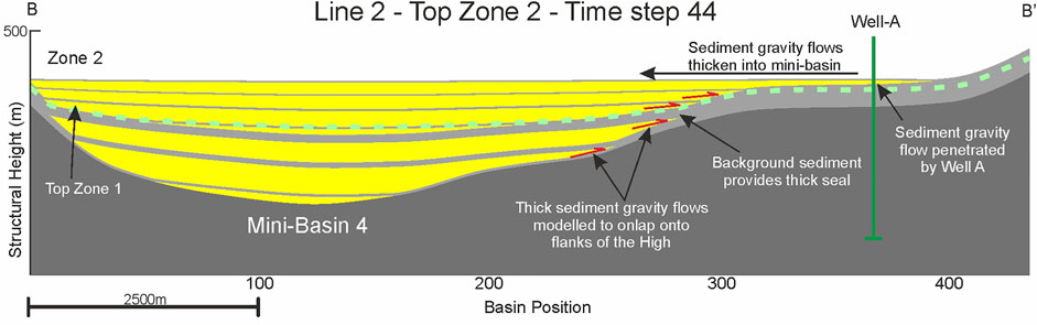
FIGURE 12. Time-Step 44 (10.0 Ma) of Line 2, showing the predicted presence of sediment gravity flows in Minibasin-1. Thick sediment gravity flows modelled in Zone 1 onlap onto the high flanks, topped by a thick laterally extensive seal of draping mudstone. Thin unit penetrated by Well-A in Zone 2 would likely have a thicker, lateral equivalent found within the basin which is what the Onlapse-2D model has simulated to develop.
How would the stratigraphy change in Minibasin-4 based on the modelling and what the well data shows us? Data from Zone 2 in Well-A is interpreted to be the distal lobe fringe of a deep-water turbidite system. The Onlapse-2D model shows packages of sediment gravity flows that thicken into the basin-axis of Minibasin-4 from Well-A in Zone 2, and thin onto and eventually onlap onto High-1. The stratal geometry here is consistent with the observations of subsurface (Mayall, et al., 2010; Doughty-Jones, et al., 2017), outcrop (Cumberpatch, et al., 2021), and numerical modelling (Sylvester, et al., 2015) of deep-water sediment gravity flows in confined tectonically active basins. These thicker sediment gravity flows could represent the sand-rich lobe axis of a confined lobe complex which progressively became unconfined through time as sediment input outpaced growth of structural accommodation. The thick deposits of the lower section of Zone 2 onlap onto the flanks of, and eventually overtop the crest of High-1 (Figure 12).
Within Zone 1 we see thick sediment gravity flows confined within Minibasin-4 that onlap onto the flank of High-1. These sediment gravity flow packages are not penetrated by Well-A, and so we cannot definitively state what the lithology of these are. Seismically we note bright to moderate amplitude continuous reflectors which can be interpreted to be a sand-prone seismic facies. This seismic facies has a morphology and scale consistent with a lobe-complex that is experiencing a strong degree of lateral confinement (sensu Prélat, Hodgson and Flint 2009; Groenenberg, et al. 2010). This interpretation is further supported by the context of the small-scale of the basin in that turbidity currents entering the basin are likely to experience a strong degree of relative confinement sensu (Stanbrook and Bentley 2021). The onlapping geometry of these sediment gravity flows represent a potential stratigraphic trap target for future consideration, and closely resembles the draping onlap (Od) described by Bakke et al. (2013). Crucially, the modelling by Onlapse-2D predicts a thick draping of background sediment, which could provide a thick laterally continuous seal for a potential stratigraphic trap target (Figure 12).
Data from Well-A indicates the presence of two condensed zones for which we have biostratigraphic age constraints. We used these to estimate the Background Sedimentation Rate, because these are regionally interpreted as condensed zones. The oldest condensed section occurred within the Middle Miocene, and gave us a rate of 0.022 mm/yr, while the youngest condensed section occurred within the Late Miocene and gave us a rate of 0.047 mm/yr, indicating a doubling of the Background Sedimentation Rate.
Lithology data from Well-A also shows that in the Late Miocene just before this doubling occurs in the background mudstone becomes considerably more carbonate-rich compared to the section below (Figure 13). We used the first appearance of a more marl-rich lithology within Well-A to give a direct indication of when the Background Sedimentation Rate should increase as Onlapse-2D does not differentiate between siliciclastic and carbonate background sediment. We interpret the cause of this increase in Background Sedimentation Rate to be an increase in carbonate productivity within the region, and this interpretation is consistent with the regional time-equivalent shelf carbonate stratigraphy. Sedimentation rates derived by Gomez Cabrera & Jackson (2009) show a marked increase in the Pliocene, which we incorporated into our Background Sedimentation Rate curve.
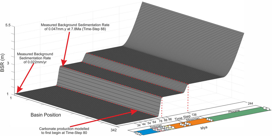
FIGURE 13. 3D representation of Background Sedimentation Rate as it evolves through time. Derived from well data from Well-A. X axis represents position in Time, showing both Time-Step and where in the chronostratigraphic column each event is. Y axis represents position along the cross-section. Z axis represents the rate of Background Sedimentation in meters.
There are marl-rich mudrocks penetrated in Zone 5 in Well-A. When we modelled these marls as background sediment, there was a significant mismatch between the seismic and the model as the Zone 5 interval extends northwards into Minibasin-4 (Figure 2); That model run predicts a thin section in the basin centre, whereas the Zone 5 seismic interval thickens into the minibasin.
Give that the well penetrated thin sediment gravity flow deposits in Zone 5 in Well-A, in a package that onlapped onto High-1 (Figure 8) we instead modelled the interval as one of active sedimentation and added a small continuous rate of rise to the Clastic Limiting Surface for that interval, which generated the observed thickening of this interval, confined to Minibasin-4. Doing so allowed us to account for differences in thicknesses observed between Well-A, and provide a better match to the subsurface data (Figure 8).
As well as the presence of marl-rich shales in this interval at Well-A, there is documentation of increases in carbonate production leading to the development of isolated carbonate build ups in shallower water sections at this time (Shann, et al., 2020). This additional line of evidence leads us to the interpretation that the modelled Gravity Flow Deposit packages which thicken northwards into Minibasin 3 in Zone 5 are likely to be calciturbidites which are derived from the shelf during this time of increased carbonate production.
What do we mean by an Informative Discrepancy? We are able to iterate towards a good solution where the model output provides a close match to the subsurface data. However, there are localized anomalies where it is not possible to iterate towards such a match using Onlapse-2D. We call these Informative Discrepancies, because they point to valuable insights. Informative Discrepancies identify places in the model where the basic assumptions of the Onlapse-2D method, do not apply; for example, no erosion or positive topography.
Our purpose with Onlapse-2D is to attain a close as match as possible between the model output and observed subsurface data. However, in this study, we demonstrate there is significant information and geological insight that can be obtained by quantifying the mismatch between the best fit model and the available data. Once we have identified an informative discrepancy, our objective shifts from attempting to make a perfect fit to making a best fit. Once this has been achieved, we can highlight the differences, quantify them, and then make a geological interpretation out of them; thereby enabling us to quantify the processes that lie outside the scope of the model. For example, we can estimate how much sediment at key points along the cross-section has been eroded, or predict the height of positive depositional topography. We believe this is a general learning that could be adopted in many other Stratigraphic Forward Modelling studies.
Overall we found the simulation produced by Onlapse-2D provided a good match to the seismic and well data. However, we found a significant mismatch on the northern flank of the High-1 in Line 1 for both Zone 3 and Zone 4 (Figure 14A). The model was simulating a significant thickness of gravity flow deposit packages when seismic data was showing us this was not the case. There was an increasing amount of over-thickening within Zone 3 and 4 extending into Minibasin-2 off of High-1, with up to 95 m of extra sediment simulated as deposited.
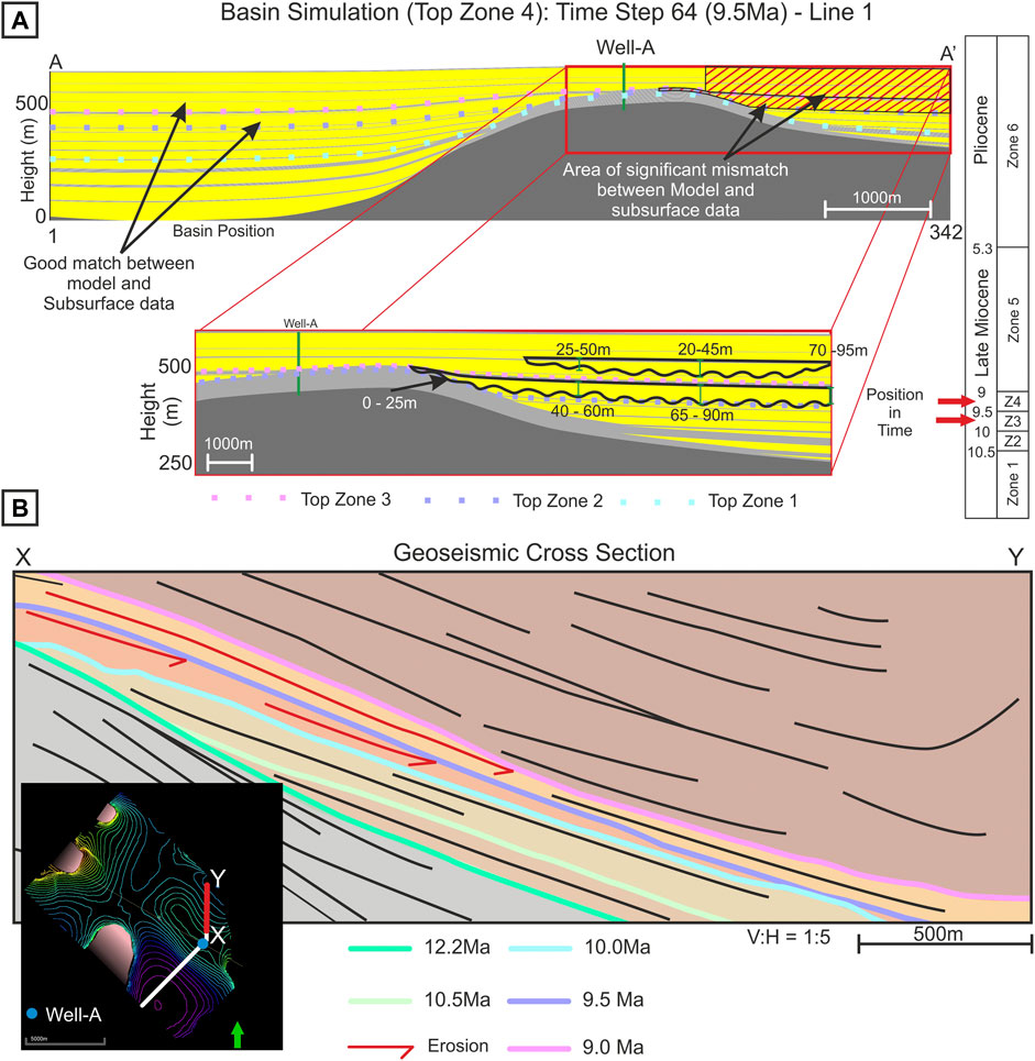
FIGURE 14. (A) Basin simulation of Top Zone 4 of Line 1. A good match was achieved between the Onlapse-2D model and subsurface data in Zone–3 & 4 in Minibasin-1 and High-1. Red hashes show in Minibasin 2 where for Zone 3 & 4 a significant mismatch occurred. Insert shows what Onlapse-2D simulated to develop, within Zone 3, an increasing amount of over-thickening is shown, and while for Zone 4 the over-thickening is more constrained to the centre of Minibasin 2. (B) Geoseismic cross section focused on Minibasin-2. Map insert shows location where geoseismic is taken from. Red arrows highlight that between 10.0–9.5 Ma & 9.5–9.0 Ma, seismic reflectors are eroded into by major horizons.This provides evidence that the mismatch between simulation and subsurface data occurs because there has been erosion within Minibasin 2.
To correct for this, we began by making iterative changes to the rate of rise of the Clastic Limiting Surface and the Structural Growth Profile, and we lowered the Initial Basin Structure for Time-Step 0. We were unable to lower the amount of over thickening in Zone 3 or 4 through these iterative changes, without substantially under-thickening the model in Well-A and in Minibasin-1 (Figure 14A). Therefore, the discrepancy is caused by a process that we do not model in the simulation (e.g. erosion or positive depositional topography).
As there is no evidence of this over thickening within our seismic, our interpretation is that there has been substantial erosion on the northern section of the High. Close inspection of the seismic data on the northern flank shows evidence of erosive features between the mapped horizons which agrees with our assessment (Figure 14B). Two laterally continuous seismic reflectors from Zone 3 which are truncated by the 9.5 ma (Top Zone 3) reflector, while another major seismic reflector from within Zone 4 is truncated by the 9.0 ma (Top Zone 4) reflector. We estimate that the amount of erosion at key points in the cross-section is from 0–25 m on High-1, up to 75–95 m in the deepest section of Minibasin-2 (Figure 14A). We believe that this erosion is caused by the major sediment fairway that in the study area, where sediment enters Minibasin-2 from the south, flows northward running axially along High-1 into Minibasin-3. Quantifying the amount of eroded section could have implications for sediment delivery to successive minibasin downslope, and possible reservoir intervals in those minibasins.
Zone 4 of Line 2 contains another major discrepancy between the modelled Onlapse-2D simulation and the subsurface data. Matching the model to seismic data and Well-A, produced over-thickening of the siliciclastic sediment deposited within the minibasin to the north-west, ranging from 60 to 102 m (Figure 15A). Quantifying the amount of eroded section could have implications for sediment delivery to successive minibasins downslope, and possible reservoir intervals in those minibasins.
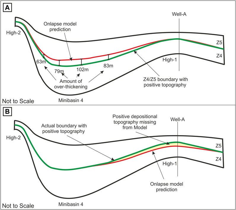
FIGURE 15. (A) Schematic diagram of mismatch between the Onlapse-2D simulation and seismic data, with significant over-thickness within Minibasin 4 from Line 2. Red horizon represents the original simulated boundary between Zone 4 & 5 within the model. Green horizon represents boundary between Zone 4 & 5 with positive depositional topography taken from seismic data. (B) Schematic diagram of Onlapse-2D in final simulation of the same line, red horizon represents Onlapse-2D simulated horizon, which now matches the boundary seen in seismic in Minibasin. From the difference between red and green horizon on High-1 we can infer the amount of positive depositional topography that is present.
Significant changes to the Structural Growth Profile, namely ceasing Fold Growth on High-1 (Figure 9) allowed us to lower this discrepancy between the model and the subsurface data. However, a discrepancy remained between the modelled simulation and the well and seismic data which we were unable to eliminate by means of further iterative changes in the inputs.
While there is evidence of erosion in Zone 3 and Zone 4 in the Line 1 seismic, close inspection of the seismic and well data provides no such evidence of erosion for either Zone in Line 2. This led us to the conclusion that positive topography (e.g. submarine lobes) found on High-1 was the cause of the significant mismatch between Onlapse-2D and the subsurface data. So we matched the thicknesses seen in Minibasin-4 instead of attempting to match the thicknesses on High-1. This provided us with a much closer fit to the subsurface data, but there was a residual discrepancy in Well-A, which allowed us to estimate how much stratigraphy was missing within the model. We can infer 5–30 m of positive depositional topography on the flanks of Minibasin-4, and at Well-A additional depositional topography of 45–70 m (Figure 15B). Data from Well-A for Zone 4 supports this interpretation with the sands encountered in the well representing sedimentation in a proximal to marginal lobes position with thick intervals of stacked amalgamated sands, consistent with the interpreted depositional topography.
This case study has demonstrated the value of a modelling software that integrates dynamic topographic development of real structures with active deposition in the evolving palaeotopography. Specifically, by seeking to precisely replicate the observed structural geometry and stratigraphic architecture, Onlapse-2D provides powerful and unexpected insights into the processes of structural and stratigraphic evolution of the study area. While this study focuses on an offshore region of the Sureste Basin, within the Gulf of Mexico we believe the workflow demonstrates the applicability of this approach in other basins with deep-water sedimentary systems such as the Northern Gulf of Mexico, offshore West Africa, or offshore Brazil.
Through the integration of both seismic and well data into the Onlapse-2D model we have been able to successfully simulate the tectonostratigraphic evolution of two cross sections across the study area in the Sureste Basin. We identified two distinct phases of compressional folding that were not parallel to each other and the long term effects of salt withdrawal and diapirism. We were able to integrate well data, age dated horizon interpretations, and seismic data to constrain and improve the modelled simulations produced by Onlapse-2D through a processes of iteration.
The best fit model for Line 2 illustrates that folding alone could not account for the stratal patterns observed in the seismic and well data and shows that structural movement resulting from salt tectonic patterns is required throughout the evolution of the cross-section. We are able to define the probable timing and rate of uplift during two distinct phases of fold growth in the Late Miocene, and this conclusion is supported by independent evidence in the timing of sand injectites. We were able to define the timing of salt withdrawal and diapirism that dominates the subsidence history in the Late Pliocene.
While we achieved a good match between the final simulation and the subsurface data for almost all intervals in both the basins modelled in the two sections, there are minor but significant intervals in which the model is unable to produce a simulation that matches the data. These model discrepancies proved to be valuable and corresponded to intervals where significant depositional topography created via erosion of previous deposits and constructional depositional topography. We term these Informative Discrepancies, and we are able to use their magnitude to quantify the amount of erosion or positive depositional topography (e.g. lobe palaeotopography) that the model software was not designed to replicate.
We have also demonstrated that the Onlapse-2D model outputs predict the distribution of potential reservoir and seal lithologies in parts of the basin away from direct well control.
The raw data supporting the conclusions of this article will be made available by the authors, without undue reservation.
DC, FP, and D“S”S contributed to the initial design and scope of the study with D“S”S organizing access to subsurface data. Modelling and analysis of results were performed by DC, with all authors contributed to further analysis of modelling results. DC wrote the first draft of the manuscript. All authors contributed to manuscript revision, read and approved the submitted version.
The work contained in this paper contains work conducted during a PhD study undertaken as part of the Natural Environment Research Council (NERC) Centre for Doctoral Training (CDT) in Oil & Gas (grant number NEM00578X/1). It is sponsored by the University of Southampton whose support is gratefully acknowledged. The University of Southampton has joined the Frontiers - JISC national open access deal and once an application form is submitted with DOI information, will be paying the submission fees.
Author D“S”S is employed by Murphy Exploration and Production Company.
The remaining authors declare that the research was conducted in the absence of any commercial or financial relationships that could be construed as a potential conflict of interest.
All claims expressed in this article are solely those of the authors and do not necessarily represent those of their affiliated organizations, or those of the publisher, the editors and the reviewers. Any product that may be evaluated in this article, or claim that may be made by its manufacturer, is not guaranteed or endorsed by the publisher.
We thank Murphy Oil Corporation for access to permission to use subsurface data, as well as their input and geological advice that was critical in this study. We would also like to thank the editorial team at Frontiers, as well reviews from Istvan Csato and Zoe Cumberpatch. Their insightful comments and suggestions were instrumental in improving this paper.
Bakke, K., Kane, I. A., Mertinsen, O. J., Petersen, S. A., Johansen, T. A., Hustoft, S., et al. (2013). Seismic Modelling in the Analysis of Deep-Water sandstone Termination Styles. AAPG Bull. 97 (9), 1395-1419. doi:10.1306/03041312069
Basani, R., Janocko, M., Cartigny, M. J. B., Hansen, E. W. M., Eggenhuisen, J. T., and Egeenhuisen, J. T. (2014). “MassFLOW-3DTM as a Simulation Tool for Turbidity Currents,” in Depositional Systems to Sedimentary Successions on the Norwegian Continental Margin. Editors A. W. Martinius, R. Ravnas, J. A. Howell, R. J. Steel, and J. P. Wonham (Chichester: International Association of Sedimentologists), Special Publication 46, 587–608. doi:10.1002/9781118920435.ch20
Burgess, P. M. (2012). A Brief Review of Developments in Stratigraphic Forward Modelling, 2000-2009. Reg. Geology. Tectonics, 378–404. doi:10.1016/b978-0-444-53042-4.00014-5
Burgess, P. M., Masiero, I., Toby, S. C., and Duller, R. A. (2019). A Big Fan of Signals? Exploring Autogenic and Allogenic Process and Product in a Numerical Stratigraphic Forward Model of Submarine-Fan Development. J. Sediment. Res. 89, 1–12. doi:10.2110/jsr.2019.3
Chand, S., Crémière, A., Lepland, A., Thorsnes, T., Brunstad, H., and Stoddart, D. (2017). Long-term Fluid Expulsion Revealed by Carbonate Crusts and Pockmarks Connected to Subsurface Gas Anomalies and Palaeo-Channels in the central North Sea. Geo-mar Lett. 37 (3), 215–227. doi:10.1007/s00367-016-0487-x
Christie, D. N. (2021).Reconstructing the Ocean Floor Shape in Turbidite Basins Using Seismic Interpretations and Forward Modelling. PhD Thesis, Southampton: School of Ocean and Earth Science, University of Southampton.
Cumberpatch, Z. A., Kane, I. A., Soutter, E. L., Hodgson, D. M., Jackson, C. A-L., Kilhams, B. A., et al. (2021). Interactinos between Deep-Water Gravity Flows and Active Salt Tectonics. J. Sediment. Res. 91, 34–65. doi:10.2110/jsr.2020.047
Davison, I., Pindell, P. J, and Hull, J. (2021). The Basins, Orogens and Evolution of the Southern Gulf of Mexico and Northern Caribbean. London: Geological Society, 1–27. doi:10.1144/sp504-2020-218
Davison, I. (2020). Salt Tectonics in the Sureste Basin, SE Mexico: Some Implications for Hydrocarbon Exploration. London: Geological Society, 147–165. doi:10.1144/SP504-2019-227
Doughty-Jones, G., Mayall, M., and Lonergan, L. (2017). Stratigraphy, Facies, and Evolution of Deep-Water Lobe Complexes within a Solt Controlled Intraslope Minibasin. AAPG Bull. 101 (11), 1879–1904. doi:10.1306/01111716046
Gomez Cabrera, P. T., and Jackson, M. P. A. (2009). “Neogene Stratigraphy and Salt Tectonics of the Santa Ana Area, Offshore Salina del Istmo Basin, Southeastern Mexico,” in Petroleum Systems in the Southern Gulf of Mexico. Editors C. Bartolini, and J. R. Román Ramos (Tulsa, Oklahoma, United States: AAPG), 237–255. doi:10.1306/13191086M9037
Granjeon, D. (2014). “3D Forward Modelling of the Impact of Sediment Transport and Base Level Cycles on continental Margins and Incised Valleys. Vol. Special Publication 46,” in From Depositional Systems to Sedimentary Successions on the Norwegian Continental Margin. Editors A. W. Martinius, R. Ravnas, J. A. Howell, R. J. Steel, and J. P. Wonham (Chichester: International Association of Sedimentologists), 453–472. doi:10.1002/9781118920435.ch16
Griffiths, C. M., Dyt, C. P., Paraschivoju, E., and Liu, K. (2001). “Sedsim in Hydrocarbon Exploration,” in Geologic Modeling and Simulation. Editors D. F. Merriam, and J. C. Davis (Boston, MA: Springer), 71–97. doi:10.1007/978-1-4615-1359-9_5
Groenenberg, R. M., Hodgson, D. M., Prélat, A., Luthi, S. M., and Flint, S. S. (2010). Flow–Deposit Interaction in Submarine Lobes: Insights from Outcrop Observations and Realizations of a Process-Based Numerical Model. J. Sediment. Res. 80 (3), 252–267. doi:10.2110/jsr.2010.028
Huang, X., Griffiths, C. M., and Liu, J. (2015). Recent Development in the Stratigraphic Forward Modelling and its Application in Petroleum Exploration. Aust. J. Earth Sci. 62, 903–919. doi:10.1080/08120099.2015.1125389
Hudec, M. R., and Norton, I. O. (2019). Upper Jurassic Structure and Evolution of the Yucatan and Campeche Subbasins, Southern Gulf of Mexico. AAPG Bull. 103 (5), 1133–1151. doi:10.1306/11151817405
Mandujano-Velazquez, J. J., and Duncan Keppie, J. (2009). Middle Miocene Chiapas Fold and Thrust belt of Mexico: a Result of Collision of the Tehuantepec Transform/Ridge with the Middle America Trench. Geol. Soc. 327, 55–69. doi:10.1144/SP327.4
Mayall, M., Lonergan, L., Bowman, A., James, S., Mills, K., Primmer, T., et al. (2010). The Response of Turbidite Slope Channels to Growth-Induced Seabed Topography. AAPG Bull. 94 (7), 1011–1030. doi:10.1306/01051009117
Padilla y Sanchez, R. J. (2007). Evolución geológica del sureste mexicano desde el Mesozoico al presente en el contexto regional del Golfo de México. Boletín de la Sociedad Geológica Mexicana 59, 19–42. doi:10.18268/BSGM2007v59n1a3
Padilla y Sanchez, R. J. (2014). Tectonics of Eastern Mexico. Search and Discovery Article #10622. AAPG Available at: http://www.searchanddiscovery.com/documents/2014/10622padilla/ndx_padilla.
Palladino, G., Grippa, A., Denis, B., Alsop, I., and Hurst, A. (2016). Emplacement of Sandstone Intrusions during Contractional Tectonics. J. Struct. Geology. 89, 230–249. doi:10.1016/j.jsg.2016.06.010
Paola, C. (2000). Quantitative Models of Sedimentary basin Filling. Sedimentology 47 (1), 121–178. doi:10.1046/j.1365-3091.2000.00006.x
Pindell, J., Weber, B., Elrich, W. H., Cossey, S., Bitter, M., Molina, R., et al. (2019). “Strontium Isotope Dating of Evaporites and the Breakup of the Gulf of Mexico and Proto-Caribbean Seaway (abs.),” in AAPG Annual Convention and Exhibition (San Antonio: AAPG).
Prélat, A., Hodgson, D. M., and Flint, S. S. (2009). Evolution, Architecture and Hierarchy of Distributary Deep-Water Deposits: a High-Resolution Outcrop Investigation from the Permian Karoo Basin, South Africa. Sedimentology 56, 2132–2154. doi:10.1111/j.1365-3091.2009.01073.x
Rivenaes, J. C. (1992). Application of Dual Lithology, Depth Dependent Diffusion Equation in Stratigraphic Simulation. Basin Res. 4, 133–146. doi:10.1111/j.1365-2117.1992.tb00136.x
Ruiz-Osorio, A. S. (2018). Tectonostratigraphic Evolution and Salt Tectonic Processes of the Isthmus Saline Basin, South-Eastern Gulf of Mexico: Implications for Petroleum Systems and Exploration. UK: Royal Holloway University of London.
Salvador, A. (1987). Late-Triassic-Jurassic Paleogeography and Origin of Gulf of Mexico Basin. AAPG Bull. 71 (4), 419–451. doi:10.1306/94886ec5-1704-11d7-8645000102c1865d
Shann, M. V., Vazquez-Reyes, K., Ali, H. M., and Horbury, A. D. (2020). The Sureste Super Basin of Southern Mexico. AAPG Bull. 104 (12), 2643–2700. doi:10.1306/09172020081
Stanbrook, D. A., Capuzzo, N., Durcanin, M., LeCompte, B., Perez, G., and Seitchik, A. (2020). “Onshore Structural Movement Revealed Through the Presence of Volcanoclastic Deposition Offshore. Cholula-1EXP, Miocene Salinas del Istmo Basin, Mexico,” in AAPG Annual Convention and Exhibition (Houston, Texas: AAPG), 18.
Stanbrook, D. S., and Bentley, M. (2021). Practical Turbidite Interpretation: The Role of Relative Confinement in Understanding Reservoir Architecture. Mar. Pet. Geology. 135, 105372. doi:10.1016/j.marpetgeo.2021.105372
Stern, R. J., and Dickinson, W. R. (2010). The Gulf of Mexico Is a Jurassic Backarc basin. Geospehere 6 (6), 739–754. doi:10.1130/GES00585.1
Sylvester, Z., Cantelli, A., and Pirmez, C. (2015). Stratigraphic Evolution of Intraslope Minibasins: Insights from Surface-Based Mode. AAPG Bull. 99 (6), 1099–1129. doi:10.1306/01081514082
Keywords: forward stratigraphic modeling, tectonostratigraphic evolution, minibasin evolution, turbidites, sediment gravity flow deposit, tectonic activity, Sureste Basin, Mexico
Citation: Christie DN, Peel FJ, Apps GM and Stanbrook D“ (2021) Forward Modelling for Structural Stratigraphic Analysis, Offshore Sureste Basin, Mexico. Front. Earth Sci. 9:767329. doi: 10.3389/feart.2021.767329
Received: 30 August 2021; Accepted: 10 November 2021;
Published: 17 December 2021.
Edited by:
Rosanna Maniscalco, University of Catania, ItalyCopyright © 2021 Christie, Peel, Apps and Stanbrook. This is an open-access article distributed under the terms of the Creative Commons Attribution License (CC BY). The use, distribution or reproduction in other forums is permitted, provided the original author(s) and the copyright owner(s) are credited and that the original publication in this journal is cited, in accordance with accepted academic practice. No use, distribution or reproduction is permitted which does not comply with these terms.
*Correspondence: Donald N. Christie, R2VvLkQuTi5DQG91dGxvb2suY29t
Disclaimer: All claims expressed in this article are solely those of the authors and do not necessarily represent those of their affiliated organizations, or those of the publisher, the editors and the reviewers. Any product that may be evaluated in this article or claim that may be made by its manufacturer is not guaranteed or endorsed by the publisher.
Research integrity at Frontiers
Learn more about the work of our research integrity team to safeguard the quality of each article we publish.