Developing an XGBoost Regression Model for Predicting Young’s Modulus of Intact Sedimentary Rocks for the Stability of Surface and Subsurface Structures

Young’s modulus (E) is essential for predicting the behavior of materials under stress and plays an important role in the stability of surface and subsurface structures. E has a wide range of applications in mining, geology, civil engineering, etc.; for example, coal and metal mines, tunnels, foundations, slopes, bridges, buildings, drilling, etc. This study developed a novel machine learning regression model, namely an extreme gradient boosting (XGBoost) to predict the influences of four inputs such as uniaxial compressive strength in MPa; density in g/cm³; p-wave velocity (Vp) in m/s; and s-wave velocity in m/s on two outputs, namely static Young’s modulus (E_s) in GPa; and dynamic Young’s modulus (E_d) in GPa. Using a series of basic statistical analysis tools, the accompanying strengths of each input and each output were systematically examined to classify the most prevailing and significant input parameters. Then, two other models i.e., multiple linear regression (MLR) and artificial neural network (ANN) were employed to predict E_s and E_d. Next, multiple linear regression and ANN were compared with XGBoost. The original dataset was allocated as 70% for the training stage and 30% for the testing stage for each model. To improve the performance of the developed models, an iterative 10-fold cross-validation method was used. Therefore, based on the results XGBoost model has revealed the best performance with high accuracy (E_s: correlation coefficient (R²) = 0.998; E_d: R² = 0.999 in the training stage; E_s: R² = 0.997; E_d: R² = 0.999 in the testing stage), root mean square error (RMSE) (E_s: RMSE = 0.0652; E_d: RMSE = 0.0062 in the training stage; E_s: RMSE = 0.071; E_d: RMSE = 0.027 in the testing stage), RMSE-standard deviation ratio (RSR) index value (E_s: RSR = 0.00238; E_d: RSR = 0.00023 in the training stage; E_s: RSR = 0.00304; E_d: RSR = 0.001 in the testing stage) and variance accounts for (VAF) (E_s: VAF = 99.71; E_d: VAF = 99.99 in the training stage; E_s: VAF = 99.83; E_d: VAF = 99.94 in the testing stage) compared to the other developed models in this study. Using a novel machine learning approach, this study was able to deliver substitute elucidations for predicting E_s and E_d parameters with suitable accuracy and runtime.

Introduction

Young’s modulus (E) is important for predicting the behavior of materials under load and plays a key part in the stability of surface and subsurface structures. E has a broad application in mining, geology, civil engineering, etc., i.e., coal and metal mines, tunnels, foundations, slopes, bridges, buildings, drilling, etc. Computation of accurate rock deformation properties, especially E is essential to the design of any rock engineering or rock mechanics project. Several researchers have studied the deformation and behavior of various types of rocks (Zhao et al., 2017; Rahimi and Nygaard, 2018; Davarpanah et al., 2019; Xiong et al., 2019). Generally, there are two common techniques, static and dynamic, employed to measure E. Static Young’s modulus (E_s) is generally acquired as the digression of the stress-strain curve at 50% of the maximum strength of the rock core sample. The dynamic Young’s modulus (E_d) can be determined if the density of the rock along with the velocities of compressional and shear waves is known. In rock engineering, the variation between E_s and E_d has been broadly investigated (Brotons et al., 2016). Normally, the value of E_d is slightly greater than the E_s studied by various researchers (Zhang, 2006; Kolesnikov, 2009). The ratio between E_d and E_s was calculated to range between 1 and 20 (Wang, 2000).

Typically, there are two common techniques, such as destructive and non-destructive, to estimate the strength and deformation of rocks. According to the recommended standards of the International Society of Rock Mechanics (ISRM) and the American Society for Testing Materials (ASTM), the use of destructive testing in the laboratory to directly estimate E is complex, time-consuming and expensive process. At the same time, sample preparation is quite difficult in the case of fragile, internally damaged, thin and highly foliated rocks (Jing et al., 2020). Thus, attention must be paid to the indirect evaluation of E through the use of rock index tests. Many researchers have established prediction models to overcome these shortcomings by employing soft computing methods such as artificial neural network (ANN), multiple regression analysis (MRA) and other novel machine learning approaches (Lindquist et al., 1994; Singh and Dubey, 2000; Tiryaki, 2008; OzcelikBayram et al., 2013; Abdi et al., 2018; Teymen and Mengüç, 2020; Cao et al., 2021; Yang et al., 2020; Duan et al., 2020). Waqas et al. used linear and nonlinear regression, regularization and ANFIS (using neuro-fuzzy inference system) to predict the E_d of sedimentary rocks (Waqas and Ahmed, 2020). Abidi et al. proposed the ANN and MRA (linear) methods for predictive modeling of E using input variables like porosity in %; dry density (γd) in g/cm³; P-wave velocity (Vp) in km/s; and water absorption (Ab) in %. The results indicated that the ANN model outperformed the MRA (Abdi et al., 2018). Davarpanah et al. developed linear and nonlinear relationships between static and dynamic deformation parameters of various rocks and found strong correlations between them (Davarpanah et al., 2020). Aboutaleb et al. conducted non-destructive experiments with SRA (simple regression analysis), MRA, ANN and SVR (support vector regression) and found that ANN and SVR models were more accurate in predicting E_d (Aboutaleb et al., 2018). Mahmoud et al. predicted the E_s of sandstone using an ANN network with 409 data events in the training phase and 183 data events in the testing phase. The developed ANN model predicted E_s with a high correlation coefficient (R² = 0.999) and minimum mean absolute percentage error (AAPE = 0.98%) (Mahmoud et al., 2019). Elkatatny developed an ANN network for predicting E_d from the drilling parameters. The study showed encouraging results (Elkatatny, 2021). Elkatatny et al. was first to correlate E_s prediction results from different models such as ANN, ANFIS and SVM. The established correlations improved the accuracy of the estimated E_s (Elkatatny et al., 2019). Cao et al. employed the novel approach of supervised machine learning, namely an extreme gradient boosting (XGBoost) combined with the firefly algorithm (FA) to predict E. The results showed that the proposed approach is suitable for predicting E.

Based on the above literature and to the best of author’s knowledge, XGBoost machine learning method has rarely been used, especially in combination with ANN and MLR, for predictive modeling of E of rocks. Due to limitations of the conventional predictive methods, the prediction of E with machine learning approaches plays a key role in determining the accuracy of the corresponding data of tests performed in the laboratory. In this novel study, XGBoost is developed for predicting E_s and E_d using four input parameters, i.e., uniaxial compressive strength (UCS) in MPa; density in g/cm³; p-wave velocity (Vp) in m/s; and s-wave velocity (Vs) in m/s, complimented with ANN and MLR. Then, the original dataset of 64 data points is split as 70% for the training stage and 30% for the testing stage. To improve the performance of the machine learning model, an iterative 10-fold cross-validation method is used.

Materials and Methods

Construction of a Dataset

Several multivariate parameters of intact sedimentary rocks (marlstone, sandstone, and limestone) are already reported (Moradian and Behnia, 2009) to have been used as inputs to predict the static Young’s modulus (E_s) and dynamic Young’s modulus (E_d), which include uniaxial compressive strength (UCS) in MPa; density in g/cm³; p-wave velocity (Vp) in m/s; and s-wave velocity (Vs) in m/s. There were a total of 64 events with no missing data. Table 1 shows the original dataset and statistical distribution in this study.

TABLE 1

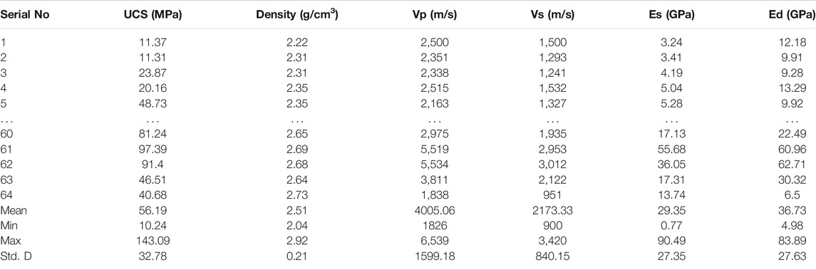
TABLE 1. Original dataset with statistical distribution in this study.

In this study, to visualize the original dataset of E, the seaborn module in Python was used. Figures 1A,B illustrate a pairwise scatter of the kernel density estimation (KDE). The purpose of building a KDE pairwise plot is to examine the association between any two influencing parameters in the original dataset. Based on Figures 1A,B, all the input parameters have a moderate to strong positive correlation with both E_s and E_d. Next, Figures 2A,B highlight the diagonal correlations between the input and output parameters. The seaborn module in Python was used for diagonal correlation heatmaps to develop the correlation coefficients of multiple inputs with E_s and E_d. Correlation coefficient values are specified in the light red to dark red color for E_s and light purple to dark purple for E_d. According to Figures 2A,B, the overall correlation coefficients between the input and output parameters are relatively high. Therefore, all parameters were incorporated to improve the accuracy of the final probabilistic prediction framework in the E_s and E_d circumstance. Figure 3 depicts the flow chart of the study.

FIGURE 1

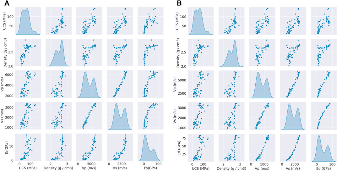
FIGURE 1. Pairwise relationship of input parameters and outputs (A) E_s and (B) E_d in the dataset.

FIGURE 2

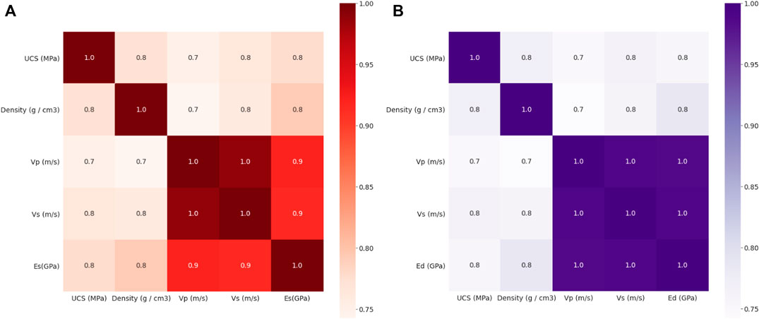
FIGURE 2. Correlation plot of input parameters and outputs (A) E_s and (B) E_d in the dataset.

FIGURE 3

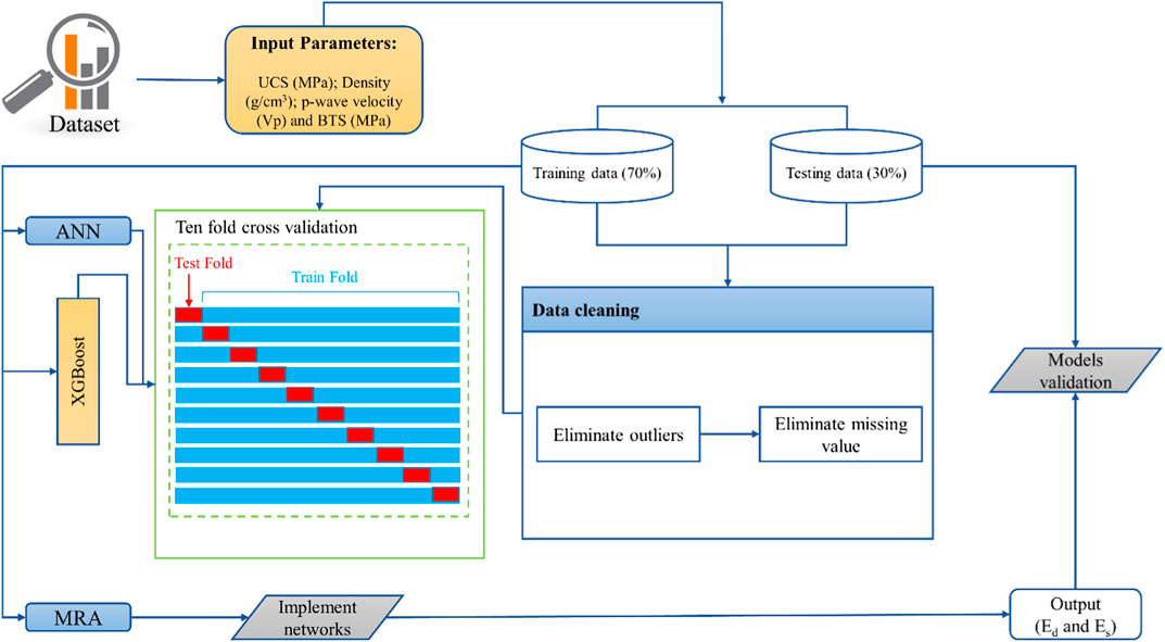
FIGURE 3. Flow chart of the study.

Methods

Multiple Regression Analysis

Multiple regression analysis (MRA) can be classified into linear and nonlinear regression. However, this study has implemented the multiple linear regression (MLR) as a result of multiple variables using SPSS (version 23). MLR is a numerical method that uses multiple descriptive parameters to estimate the output of a reporting parameter. The MLR method is used to obtain the best-fit relationship between the parameters. Generally, MLR can be employed to establish the association between independent (input) and dependent (output) parameters. In this study, the MLR technique was used to predict E_s and E_d, respectively. The MLR relationship between the inputs and output can usually be expressed by Eq. 1.

$D=a+B_1{X}_1+B_2{X}_2+B_3{X}_3+\dots +B_n{X}_n(1)$

where, D depicts the output parameter, $a$ denotes the regression constant, $B_1$–$B_n$ are the coefficients of regression and $X_1$–$X_n$ are the input variables.

Based on the consequences of MLR, E_s and E_d are predicted by the established linear expressions as shown in Eqs 2, 3.

$E_s=0.086UCS+26.55Density+0.014Vp-0.004Vs-89.47(2)$

$E_d=14.568Density+0.008Vp-0.15Vs-0.034UCS-64(3)$

where, $E_s$ and $E_d$ are static and dynamic Young’s modulus in GPa, respectively. UCS represents uniaxial compressive strength in MPa, Vp and Vs are the p-wave and s-wave velocities in m/s, respectively.

Artificial Neural Network

Artificial neural network (ANN) is among many supervised machine learning methods and has found wide application in a variety of fields. An ANN consists of three components, i.e., input layers, hidden layers, and an output layer. The structure of ANN and the choice of hidden layers and neurons play a crucial part in ascertaining its performance (Chester, 1990). The feedforward back-propagation (FFBP) neural network, a multilayer perceptron network, was used owing to its simple process and wide applicability. Back-propagation (BP) is one of the most efficient and commonly employed learning algorithms in multi-layer networks (Cevik et al., 2011; Hajihassani et al., 2014). Each network must contain sufficient neurons depending on the application of ANN. Neurons of a given layer are connected to the neurons of the subsequent consecutive layer with every connection having a certain weightage (Atkinson and Tatnall, 1997). Equation 4 is employed to estimate the approximate number of neurons in the hidden layer ($N_h$), since the inappropriate selection of the neurons in the hidden layer often leads to “under-fitting” and “over-fitting” and must be prevented. Figure 4 represents the basic structure of the ANN network for predicting E_s and E_d in this study.

$N_h\le 2N_1+1(4)$

where, N₁ denote the total number of inputs.

FIGURE 4

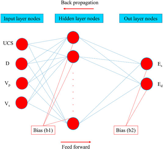
FIGURE 4. Basic architecture of ANN network.

In order to build the net input n, the weighted input ${\omega }_i{\text{p}}_i$ is connected to a scalar bias$b$, $f$ denotes the transfer function, and $O$ denotes the scalar output. If the neuron has Z input parameters, the output can be computed by Eq. 5.

$O=f{\sum }_{i=1}^Z\left({\omega }_i{\text{p}}_i+b\right)(5)$

This study used a sigmoid transfer function in the hidden layer and a linear output function in the output layer. To achieve the number of neurons in the hidden layer, this study used some provisions, since there is no specific approach to providing the desired results. In addition, fifty epochs were used for training the ANN network and the least error of validation is considered as a stop to avoid overfitting.

Extreme Gradient Boosting

The extreme gradient boosting (XGBoost) algorithm was created by Chen and Guestrin (Chen and Guestrin, 2016). Being an effective tree-based ensemble learning algorithm, it is considered a powerful tool among data science researchers. XGBoost is based on gradient boosting architecture (Friedman, 2001), which uses various complement functions to estimate the results using Eq. 6.

$\overline{y_i}= y_i^0+\eta {\sum }_{K=1}^n{f}_k\left(U_i\right) (6)$

where, $\overline{y_i}$ indicates the predicted output for $i$th data with the parameter vector $U_i$; n denotes the number of estimators corresponding to independent tree structures for each f_k (i.e. k = 1 to n); and $y_i^0$ displays the primary hypothesis, which is actually the mean of the original parameters in the training data. $\eta$ represents the rate of learning connected to improving the performance of the model, whether connecting the additional trees to prevent over-fitting. The statistical model has to be developed with less overfitting which is one of the genuine problems that often conflicts in machine learning. In the XGBoost model, the training phase is determined in a complementary way.

According to Eq. 3 in the kth stage, the kth estimator is connected to the model and the prediction of the kth $y_i^{-k}$ is calculated from the estimated output $y_i^{-(k-1)}$ in the next step, and the established f_k of the kth complementary estimator is shown in Eq. 7.

$y_i^{-k}=y_i^{-\left(k-1\right)}+ \eta f_k (7)$

whereas $f_k$ represents the leaves weight that is established by reducing the objective function of the kth tree and is given by Eq. 8.

$f_{obj}= \gamma Z + {\sum }_{a=1}^Z[ g_a{\omega }_a+ \frac{1}{2} \left(h_a+ \lambda \right) {\omega }_a^2 (8)$

where, Z denotes the quantity of leaf nodes, $\gamma$ denotes the complexity parameter, $\lambda$ denotes constant coefficient, and ${\omega }_a^2$ denotes the leaf weight from 1 to Z. $\gamma$ and $\lambda$ are regularization parameters employed to improve the model to keep away from the over-fitting. $g_a$ and $h_a$ are the summation parameters for the entire dataset associated with a leaf of the initial and previous loss function gradient, correspondingly. In order to build the kth tree, a leaf is distributed into several leaves. Such a system is implied by using the gain parameters expressed in Eq. 9.

$G= \frac{1}{2} \left[\frac{O_L^2}{P_L+ \lambda }+ \frac{O_R^2}{P_R+ \lambda } + \frac{ {\left(O_L+ O_R\right)}^2}{P_L+ P_R + \lambda }\right](9)$

where, G denotes the gain parameters, $O_R$ and $P_R$ denote the right leaf, respectively. $O_L$ and $P_L$denote the subsequent division of the left leaf, respectively. When the gain parameter is approximated to zero, the division criteria are generally assumed. $\gamma$ and $\lambda$ are regularization parameters that are indirectly reliant on the gain parameters. For example, a larger regularization parameter can significantly reduce the gain parameter, thus avoiding the leaf convolution phenomenon. However, this will reduce the performance of the model to adapt to the training data. Figure 5A demonstrates the basic structure of the level-wise XGBoost tree model.

FIGURE 5

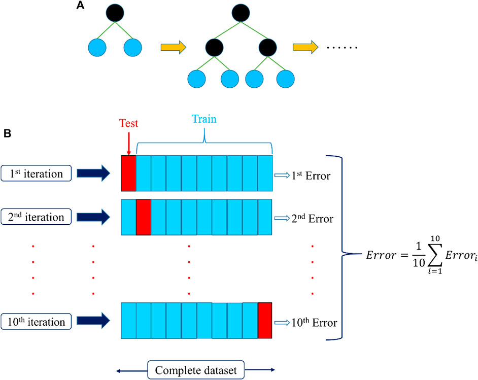
FIGURE 5. (A) Basic structure of the level-wise XGBoost tree model. (B) Grid search cross validation.

Grid Search Cross Validation

The grid search method is used for the adjustment of hyperparameters (Bergstra and Bengio, 2012). The technique approves a search in an identified range of hyperparameters and defines the desired results leading to the best outcomes of the assessment criteria, i.e., R², MAE, MSE and RMSE. GridSearchCV() has been carried out in scikit-learn Python programing language to process this strategy. This method simply calculates the score of CV for all hyperparameters integrated with a particular reach. In this study, a 10-fold iterated arbitrary arrangement practice was incorporated in the CV command as specified in Figure 5B. GridSearchCV() allows not only to compute the desired hyperparameters, but also to evaluate the metric values to their desired outcomes. This study used all the remaining features of the Python programing language by default to perform Grid Search CV.

Performance Criterion

Typically, the performance of a model must be estimated when approaching the steadiness of a prediction framework, using an extensive range of performance criteria to select a highly accurate model. Therefore, this study proposes a unique performance criterion as follows:

Correlation coefficient

The correlation coefficient (R²) is the key to the execution of the regression survey. The computation of R² can be expressed by Eq. 10.

$R^2=\frac{{{\displaystyle \sum }}_{i=1}^n\left(Xi-\overline{X}\right)\left(Yi-\overline{Y}\right)}{{\sqrt{{{\displaystyle \sum }}_{i=1}^n{\left(Xi-\overline{X}\right)}^2\left(Yi-\overline{Y}\right)}}^2}(10)$

Mean Square Error

Mean square error (MSE) is the mean of the square of all errors and is one of the important metrics for evaluating the performance of the corresponding models. The computation of MSE can be expressed by Eq. 11.

$MSE=\frac{{{\displaystyle \sum }}_{i=1}^n{\left(Xi-Yi\right)}^2}{n}(11)$

Root Mean Square Error

Root mean square error (RMSE) is the square root of the mean of the square of all errors and is measured as significant metric for mathematical predictions. The computation of RMSE can be expressed by Eq. 12.

$RMSE=\sqrt{\frac{{{\displaystyle \sum }}_{i=1}^n{\left(Xi-Yi\right)}^2}{n}}(12)$

Root Mean Square Error Standard Deviation Ratio

Root Mean Square Error Standard Deviation Ratio (RSR) is employed in this study for the comparison of significant models, which can be executed to predict E_s and E_d. RSR plays an important role as a valuable metric for testing analytical models. The computation of RSR can be expressed by Eq. 13.

$RSR=\frac{\sqrt{{{\displaystyle \sum }}_{i=1}^n{\left(Xi-Yi\right)}^2}}{\sqrt{{{\displaystyle \sum }}_{i=1}^n{\left(Xi-\overline{Yi}\right)}^2}}(13)$

Variance Accounts For

Variance accounts for (VAF) is also considered as one of the important metrics for evaluating the overall performance of the model. Higher the VAF value, the greater will be the performance of the model. The computation of VAF can be expressed by Eq. 14.

$VAF=\left[1-\frac{var\left(Xi-Yi\right)}{var\left(Xi\right)}\right]\times 100(14)$

where, $\overline{X}$ and $\overline{Y}$ are the mean of the original and predicted data values, respectively, $X_i$ and $Y_i$ are the original and predicted data values, respectively, and n shows the number of datasets. $\overline{Yi}$ is the mean value of the original data. Table 2 signifies the performance ranking and the corresponding RSR values.

TABLE 2

TABLE 2. Performance ranking and the corresponding RSR index values.

Results and Discussion

In this study, a novel machine learning regression XGBoost model was developed and compared with two other models, namely MLR and ANN, to confirm the accuracy of predicting E_s and E_d. To avoid overfitting of these models, the original dataset was partitioned into 70% for the training stage and 30% for the testing stage of 64 events. The ANN and XGBoost models are trained on training data and then validated by testing data. The 50 epochs were used for training the ANN model and the least error of validation is considered as a stop to avoid overfitting. According to Eq. 4, a total of nine neurons are selected in the hidden layer, which is connected to four input neurons and two output neurons, as shown in Figure 4. In this study, an XGBoost model with the default features of the XGBoost module was executed, i.e., M = 50 estimators, the regularization properties of γ = 0, λ = 1, and a learning rate of η = 0.3. Moreover, a 10-fold iterated arbitrary arrangement practice was incorporated to substantiate the models.

The original and predicted output values were then arranged and represented in scattered plots in order to ease the performance and correlation analysis of the developed models. The input parameters are UCS (MPa); Density (g/cm³); Vp (m/s); and Vs (m/s). The predicted output parameters are E_s and E_d. The final output was evaluated by using performance criteria such as R², RMSE and VAF, and the developed models were compared to estimate the appropriate model with higher accuracy of prediction results in this study.

Figures 6A,B to Figures 7A,B depict the scatter plots of the predictions of the proposed models (a) MLR, (b) ANN and (c) XGBoost for E_s and E_d versus the original data in the training and testing stages, respectively. The prediction performance accuracy of the proposed models is (a) MRA (E_s: R² = 0.928; E_d: R² = 0.981 in the training stage, and; E_s: R² = 0.717; E_d: R² = 0.985 in the testing stage), (b) ANN (E_s: R² = 0.958; E_d: R² = 0.998 in the training stage; and E_s: R² = 0.849; E_d: R² = 0.998 in the testing stage) and (c) XGBoost (E_s: R² = 0.998; E_d: R² = 0.999 in the training stage, and; E_s: R² = 0.997; E_d: R² = 0.999 in the testing stage).

FIGURE 6

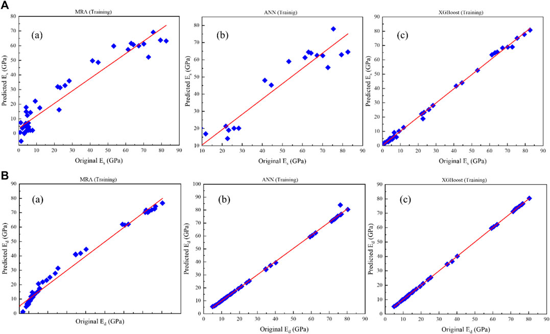
FIGURE 6. Results of (A) E_s and (B) E_d prediction against original data in the training stage: (a) MLR, (b) ANN, and (c) XGBoost.

FIGURE 7

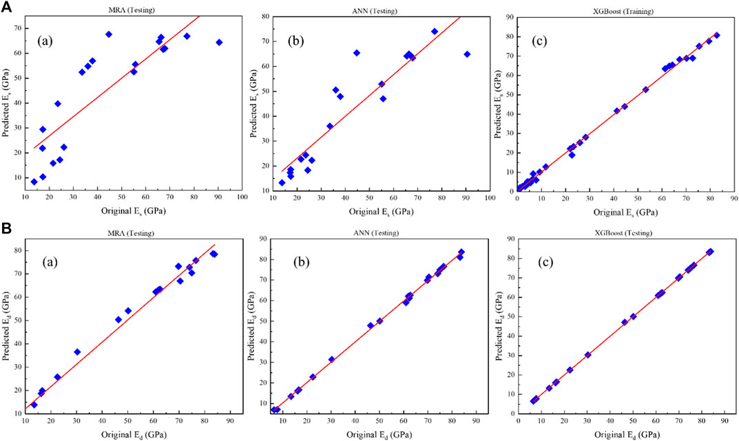
FIGURE 7. Results of (A) E_s and (B) E_d prediction against original data in the testing stage: (a) MLR, (b) ANN, and (c) XGBoost.

Simultaneously, to comprehend the good visualization of the predicted values aggregated with the original data of E_s and E_d, Figures 8A,B demonstrate the performance of MLR, ANN and XGBoost models in the training stage, respectively. Figures 9A,B demonstrate the performance of MLR, ANN and XGBoost models in the testing stage for (a) E_s and (b) E_d, respectively.

FIGURE 8

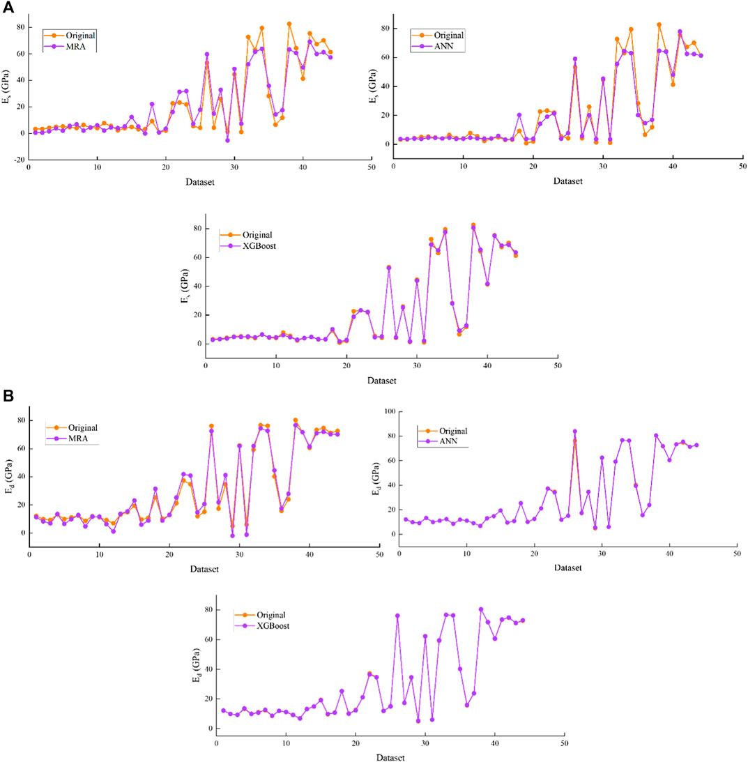
FIGURE 8. Demonstration of predicted against original data of proposed models in the training stage for (A) E_s and (B) E_d.

FIGURE 9

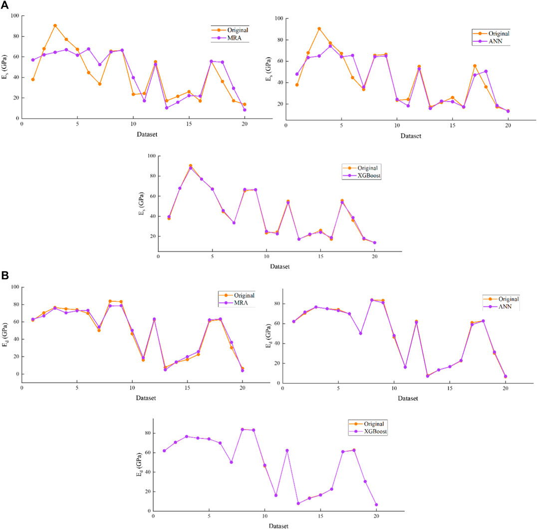
FIGURE 9. Demonstration of predicted against original data of proposed models in the testing stage for (A) E_s and (B) E_d.

Figures 10A,B demonstrates the variation of the relative error of the proposed models, i.e., MLR, ANN, and XGBoost, for the prediction of E_s and E_d and the original data in (a) training stage and (b) testing stage, respectively. The prediction performance of the proposed models for variation in relative mean square error (MSE) is (a) MLR (E_s: MSE = 0.095; E_d: MSE = 0.00014 in the training stage, and; E_s: MSE = 2.617; E_d: MSE = 0.079 in the testing stage), (b) ANN (E_s: MSE = 1.009; E_d: MSE = 0.030 in the training stage, and; E_s: MSE = 0.278; E_d: MSE = 0.079 in the testing stage) and (c) XGBoost (E_s: MSE = 0.0043; E_d: MSE = 0.00003 in the training stage, and; E_s: MSE = 0.0051; E_d: MSE = 0.0007 in the testing stage).

FIGURE 10

FIGURE 10. Change of relative error between predicted and original data of proposed models in the (A) training stage and (B) testing stage for E_s and E_d.

Table 3 shows the performance criterion of the MRA, ANN and XGBoost determined using Eq. 10–14. Figure 11 depicts the comparative Taylor diagrams of the proposed models MRA, ANN and XGBoost in the (a) training stage and (b) testing stage for E_s and E_d to further estimate the performance of the models more extensively. The standard deviation values associated with one another by the circular lines are shown as horizontal and vertical coordinates in the diagrams. Two performance metrics, one is the R² value, indicated by the blue radial lines from the starting of the coordinates, and the other is the RMSE value, specified by the green circular line. Observed values were used as the base model with zero errors, i.e., RMSE = 0 in the diagrams, the maximum R² = 1, and the computed standard deviations. Next, the R², RMSE and standard deviation of the other models were compared with the observed values. A best model is one with highest degree of similarity to observed data model. As shown in Figure 11, the XGBoost model has been able to approach the observed data and outperformed the MRA and ANN models in both the training and testing phases.

TABLE 3

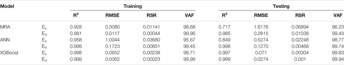
TABLE 3. Performance criterion of the MRA, ANN, and XGBoost.

FIGURE 11

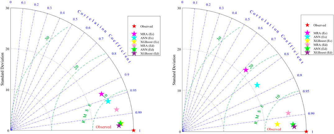
FIGURE 11. The comparative Taylor diagrams of the proposed models MRA, ANN, and XGBoost in the (A) training stage and (B) testing stage for E_s and E_d.

Moreover, according to Table 3 and the results in Figure 11, the XGBoost model has revealed the best performance with high accuracy (E_s: R² = 0.998; E_d: R² = 0.999 in the training stage, and; E_s: R² = 0.997; E_d: R² = 0.999 in the testing stage), RMSE (E_s: RMSE = 0.0652; E_d: RMSE = 0.0062 in the training stage, and; E_s: RMSE = 0.071; E_d: RMSE = 0.027 in the testing stage), RSR index value (E_s: RSR = 0.00238; E_d: RSR = 0.00023 in the training stage, and; E_s: RSR = 0.00304; E_d: RSR = 0.001 in the testing stage) and VAF (E_s: VAF = 99.71; E_d: VAF = 99.99 in the training stage, and; E_s: VAF = 99.83; E_d: VAF = 99.94 in the testing stage) compared to the other developed models in this study.

Therefore, XGBoost is an applicable machine learning regression model that can be applied to accurately predict the E_s and E_d.

Conclusion

Young’s modulus (E) plays an important role in the stability of surface and subsurface structures. Therefore, an accurate estimation of E is mandatory. This study developed a novel machine learning XGBoost regression model with four input parameters, i.e., UCS (MPa), density (g/cm³), Vp (m/s) and Vs (m/s) for predicting E_s (GPa) and E_d (GPa). In addition, the MRA and ANN models were included to compare their results with the proposed model. To avoid overfitting of these models, the original dataset was partitioned into 70% for the training stage and 30% for the testing stage of 64 data points. The study concludes that the proposed XGBoost regression model performed more accurately than the other studied models in predicting E_s and E_d. Employing a novel machine learning approach, this study was able to provide substitute elucidations to predict E_s and E_d parameters with appropriate accuracy and runtime. Future work can be extended using various datasets to further confirm the reliability of the proposed model.

Data Availability Statement

The original contributions presented in the study are included in the article/Supplementary Material, further inquiries can be directed to the corresponding author.

Author Contributions

NS: Conceptualization, Methodology, Writing Original Draft, and Run Code. XZ: Project Supervisor, Funding, and Review and Editing. CL: Run Code and Visualization. FH: Review and Editing. PL: Data Curation and Run Code.

Funding

This research was supported by the Science and Technology Innovation Project of Guizhou Province (Qiankehe Platform Talent (2019) 5620 to XZ). No additional external funding was received for this study.

Conflict of Interest

XZ was employed by Guizhou Guineng Investment Co., Ltd.

The remaining authors declare that the research was conducted in the absence of any commercial or financial relationships that could be construed as a potential conflict of interest.

Publisher’s Note

All claims expressed in this article are solely those of the authors and do not necessarily represent those of their affiliated organizations, or those of the publisher, the editors and the reviewers. Any product that may be evaluated in this article, or claim that may be made by its manufacturer, is not guaranteed or endorsed by the publisher.

References

Abdi, Y., Garavand, A. T., and Sahamieh, R. Z. (2018). Prediction of Strength Parameters of Sedimentary Rocks Using Artificial Neural Networks and Regression Analysis. Arabian J. Geosci. 11 (19), 1–11. doi:10.1007/s12517-018-3929-0

CrossRef Full Text | Google Scholar

Aboutaleb, S., Behnia, M., Bagherpour, R., and Bluekian, B. (2018). Using Non-destructive Tests for Estimating Uniaxial Compressive Strength and Static Young's Modulus of Carbonate Rocks via Some Modeling Techniques. Bull. Eng. Geol. Environ. 77 (4), 1717–1728. doi:10.1007/s10064-017-1043-2

CrossRef Full Text | Google Scholar

Atkinson, P. M., and Tatnall, A. R. L. (1997). Introduction Neural Networks in Remote Sensing. Int. J. Remote Sensing 18 (4), 699–709. doi:10.1080/014311697218700

CrossRef Full Text | Google Scholar

Bergstra, J., and Bengio, Y. (2012). Random Search for Hyper-Parameter Optimization. J. Machine Learn. Res. 13 (2), 281–305. doi:10.1016/j.chemolab.2011.12.002

CrossRef Full Text | Google Scholar

Brotons, V., Tomás, R., Ivorra, S., Grediaga, A., Martínez-Martínez, J., Benavente, D., et al. (2016). Improved Correlation between the Static and Dynamic Elastic Modulus of Different Types of Rocks. Mater. Struct. 49 (8), 3021–3037. doi:10.1617/s11527-015-0702-7

CrossRef Full Text | Google Scholar

Cao, J., Gao, J., Rad, H. N., Mohammed, A. S., Hasanipanah, M., and Zhou, J. (2021). A Novel Systematic and Evolved Approach Based on XGBoost-Firefly Algorithm to Predict Young’s Modulus and Unconfined Compressive Strength of Rock. Eng. Comput. doi:10.1007/s00366-020-01241-2 Published online

CrossRef Full Text | Google Scholar

Cevik, A., Sezer, E. A., Cabalar, A. F., and Gokceoglu, C. (2011). Modeling of the Uniaxial Compressive Strength of Some clay-bearing Rocks Using Neural Network. Appl. Soft Comput. 11 (2), 2587–2594. doi:10.1016/j.asoc.2010.10.008

CrossRef Full Text | Google Scholar

Chen, T., and Guestrin, C. (2016). “Xgboost: A Scalable Tree Boosting System,” in Proceedings of the 22nd Acm Sigkdd International Conference on Knowledge Discovery and Data Mining, San Francisco, CA, August 13–17, 2016, 785–794.

Google Scholar

Chester, D. L. (1990). “Why Two Hidden Layers Are Better Than One,” in Proceeding of IJCNN (Washington, DC), 1, 265–268.

Google Scholar

Davarpanah, M., Somodi, G., Kovács, L., and Vásárhelyi, B. (2019). Complex Analysis of Uniaxial Compressive Tests of the Mórágy Granitic Rock Formation (Hungary). Stud. Geotechn. et Mech. 41 (1), 21. doi:10.2478/sgem-2019-0010

CrossRef Full Text | Google Scholar

Davarpanah, S. M., Ván, P., and Vásárhelyi, B. (2020). Investigation of the Relationship between Dynamic and Static Deformation Moduli of Rocks. Geomech. Geophys. Geo-Energy Geo-Res. 6 (1), 1–14. doi:10.1007/s40948-020-00155-z

CrossRef Full Text | Google Scholar

Duan, J., Asteris, P. G., Nguyen, H., Bui, X. N., and Moayedi, H. (2020). A Novel Artificial Intelligence Technique to Predict Compressive Strength of Recycled Aggregate concrete Using ICA-XGBoost Model. Eng. Comput. 37, 1–18. doi:10.1007/s00366-020-01003-0

CrossRef Full Text | Google Scholar

Elkatatny, S. (2021). Real-Time Prediction of the Dynamic Young’s Modulus from the Drilling Parameters Using the Artificial Neural Networks. Arabian J. Sci. Eng.. doi:10.1007/s13369-021-05465-2 Published online

CrossRef Full Text | Google Scholar

Elkatatny, S., Tariq, Z., Mahmoud, M., Abdulraheem, A., and Mohamed, I. (2019). An Integrated Approach for Estimating Static Young's Modulus Using Artificial Intelligence Tools. Neural Comput. Applic. 31 (8), 4123–4135. doi:10.1007/s00521-018-3344-1

CrossRef Full Text | Google Scholar

Friedman, J. H. (2001). Greedy Function Approximation: a Gradient Boosting Machine. Ann. Stat., 1189–1232. doi:10.1214/aos/1013203451

CrossRef Full Text | Google Scholar

Hajihassani, M., Jahed Armaghani, D., Sohaei, H., Tonnizam Mohamad, E., and Marto, A. (2014). Prediction of Airblast-Overpressure Induced by Blasting Using a Hybrid Artificial Neural Network and Particle Swarm Optimization. Appl. Acoust. 80, 57–67. doi:10.1016/j.apacoust.2014.01.005

CrossRef Full Text | Google Scholar

Jing, H., Rad, H. N., Hasanipanah, M., Armaghani, D. J., and Qasem, S. N. (2020). Design and Implementation of a New Tuned Hybrid Intelligent Model to Predict the Uniaxial Compressive Strength of the Rock Using SFS-ANFIS. Eng. Comput. 37, 1–18. doi:10.1007/s00366-020-00977-1

CrossRef Full Text | Google Scholar

Kolesnikov, Y. I. (2009). Dispersion Effect of Velocities on the Evaluation of Material Elasticity. J. Min. Sci. 45 (4), 347–354. doi:10.1007/s10913-009-0043-4

CrossRef Full Text | Google Scholar

Lindquist, E. S., and Goodman, R. E. (1994). “Strength and Deformation Properties of a Physical Model Melange,” in Proceedings of the 1st North American Rock Mechanics Symposium. Editors P. P. Nelson, and SE. Laubach (Rotterdam: Balkema).

Google Scholar

Mahmoud, A. A., Elkatatny, S., Ali, A., and Moussa, T. (2019). Estimation of Static Young's Modulus for Sandstone Formation Using Artificial Neural Networks. Energies 12 (11), 2125. doi:10.3390/en12112125

CrossRef Full Text | Google Scholar

Moradian, Z. A., and Behnia, M. (2009). Predicting the Uniaxial Compressive Strength and Static Young's Modulus of Intact Sedimentary Rocks Using the Ultrasonic Test. Int. J. Geomech. 9 (1), 14–19. doi:10.1061/(asce)1532-3641(2009)9:1(14)

CrossRef Full Text | Google Scholar

OzcelikBayram, Y. F., Bayram, F., and Yasitli, N. E. (2013). Prediction of Engineering Properties of Rocks from Microscopic Data. Arab J. Geosci. 6, 3651–3668. doi:10.1007/s12517-012-0625-3

CrossRef Full Text | Google Scholar

Rahimi, R., and Nygaard, R. (2018). Effect of Rock Strength Variation on the Estimated Borehole Breakout Using Shear Failure Criteria. Geomech. Geophys. Geo-Energ. Geo-Resour. 4 (4), 369–382. doi:10.1007/s40948-018-0093-7

CrossRef Full Text | Google Scholar

Singh, T. N., and Dubey, R. K. (2000). A Study of Transmission Velocity of Primary Wave (P-Wave) in Coal Measures sandstone. J. Scientific Ind. Res. 59, 482–486. doi:10.1361/105497100770340147

CrossRef Full Text | Google Scholar

Teymen, A., and Mengüç, E. C. (2020). Comparative Evaluation of Different Statistical Tools for the Prediction of Uniaxial Compressive Strength of Rocks. Int. J. Mining Sci. Techn. 30 (6), 785–797. doi:10.1016/j.ijmst.2020.06.008

CrossRef Full Text | Google Scholar

Tiryaki, B. (2008). Predicting Intact Rock Strength for Mechanical Excavation Using Multivariate Statistics, Artificial Neural Networks, and Regression Trees. Eng. Geol. 99, 51–60. doi:10.1016/j.enggeo.2008.02.003

CrossRef Full Text | Google Scholar

Wang, Z. (2000). Dynamic versus Static Elastic Properties of Reservoir Rocks. Seismic Acoust. Velocities Res. Rocks 3, 531–539.

Google Scholar

Waqas, U., and Ahmed, M. F. (2020). Prediction Modeling for the Estimation of Dynamic Elastic Young's Modulus of Thermally Treated Sedimentary Rocks Using Linear-Nonlinear Regression Analysis, Regularization, and ANFIS. Rock Mech. Rock Eng. 53 (12), 5411–5428. doi:10.1007/s00603-020-02219-8

CrossRef Full Text | Google Scholar

Xiong, L. X., Xu, Z. Y., Li, T. B., and Zhang, Y. (2019). Bonded-particle Discrete Element Modeling of Mechanical Behaviors of Interlayered Rock Mass under Loading and Unloading Conditions. Geomech. Geophys. Geo-Energ. Geo-Resour. 5 (1), 1–16. doi:10.1007/s40948-018-0090-x

CrossRef Full Text | Google Scholar

Yang, F., Li, Z., Wang, Q., Jiang, B., Yan, B., Zhang, P., et al. (2020). Cluster-formula-embedded Machine Learning for Design of Multicomponent β-Ti Alloys with Low Young’s Modulus. npj Comput. Mater. 6 (1), 1–11. doi:10.1038/s41524-020-00372-w

CrossRef Full Text | Google Scholar

Zhang, L. (2006). Engineering Properties of Rocks. Lexington: Univ of Kentucky.

Google Scholar

Zhao, Y. S., Wan, Z. J., Feng, Z. J., Xu, Z. H., and Liang, W. G. (2017). Evolution of Mechanical Properties of Granite at High Temperature and High Pressure. Geomech. Geophys. Geo-Energ. Geo-Resour. 3 (2), 199–210. doi:10.1007/s40948-017-0052-8

CrossRef Full Text | Google Scholar