High-Performance Computing of 3D Magma Dynamics, and Comparison With 2D Simulation Results

The dynamics of magma is often studied through 2D numerical simulations because 3D simulations are usually complex and computationally expensive. However, magmatic systems and physical processes are 3D and approximating them in 2D requires an evaluation of the information which is lost under different conditions. This work presents a physical and numerical model for 3D magma convection dynamics. The model is applied to study the dynamics of magma convection and mixing between andesitic and dacitic magmas. The 3D simulation results are compared with corresponding 2D simulations. We also provide details on the numerical scheme and its parallel implementation in C++ for high-performance computing. The performance of the numerical code is evaluated through strong scaling exercises involving up to $>$12,000 cores.

1 Introduction

Understanding magma transport in the crust is one of the major challenges in modern volcanology. Current models depict magmatic systems as an interconnected network of compositionally heterogeneous magmas, involving multiple chambers and dikes that extend from shallow to deep levels in the crust (Gudmundsson, 1995; Gudmundsson, 2011; Blundy and Annen, 2016).

Magma chambers are the main engines of active volcanoes and serve as a storage region for magma ascent and its chemical evolution (DePaolo, 1981; Bachmann and Bergantz, 2003). The pressure in the chamber may vary largely over time due to a variety of processes, including fractional crystallization, volatile exsolution and magma recharge, potentially leading towards an eruption (Sparks and Huppert, 1984; Folch and Marti, 1998; Gudmundsson, 2012; Edmonds and Wallace, 2017; Papale et al., 2017; Cassidy et al., 2018). Therefore, studying magma dynamics in a chamber is of utmost importance and has become a mainstream theme over the recent years (Bergantz, 2000; Couch et al., 2001; Gutiérrez and Miguel, 2010; Karlstrom et al., 2010; Bergantz et al., 2015; Garg et al., 2019) as the ongoing flow dynamics and associated surface signals can depict the current state of the volcano and its possible evolutions (Gottsmann et al., 2011; Longo et al., 2012a; Bagagli et al., 2017; Sparks and Cashman, 2017; Carrara, 2019; Lieto et al., 2020).

Typically, buoyancy instabilities develop when a low-density, volatile-rich, primitive, hot magma ascends in the crust and interacts with previously stored, more chemically evolved, partially degassed and denser magma in shallow chambers (Semenov and Polyansky, 2017; Garg et al., 2019). There are multiple pieces of evidence of eruptions shortly preceded by interaction of compositionally different magmas at shallow depths (Tomiya et al., 2013; Sides et al., 2014; Perugini et al., 2015; Sundermeyer et al., 2020). The degree of magma mixing, which spans a continuum from mechanical mingling to complete chemical homogenisation, depends upon the magma properties, the driving forces, and the time available for mixing (Garg et al., 2019).

Recently a number of authors [e.g., (Sparks and Cashman, 2017), and references therein] have been hypothesizing that although usually not seen among the erupted volcanic products, a crystal-rich mush may constitute a large dominant portion of the magmatic plumbing system, with dominantly liquid magma possibly being an ephemeral occurrence driven by melt segregation and contributing to characterize the unrest and eruption states of the volcano. Clear evidence from active magmatic systems is not available yet, as volcanic plumbing systems continue to be hidden from direct observation. A few accidental encounters with buried shallow magma bodies during geothermal drilling do not appear to support the presence of important layers of mushy magma across the rock-magma transition (Eichelberger, 2020). More is needed before we get to a clear, robust picture of active magmatic systems, justifying substantial efforts to overcome the current limitations in directly observing, measuring and sampling underground magma (https://www.kmt.is). Here we focus on either dominantly liquid reservoirs, or on the dominantly liquid core region of mushy magma reservoirs, over time scales that are typical of individual magma convection events, likely much less than the time scales associated with the existence of ephemeral liquid-dominated magmatic bodies.

Over the years significant efforts have been invested to study several aspects of the magma physics relevant to understand the volcano dynamics and anticipate their evolution. The physics of magma mixing has been studied through numerical simulations and experiments with both synthetic and natural compositions (Campbell and Turner, 1986; Huppert et al., 1986; Jellinek and Kerr, 1999; Michioka and Sumita, 2005; Sato and Sato, 2009; De Campos et al., 2011; Laumonier et al., 2014; Morgavi et al., 2015; Perugini et al., 2015; Bergantz et al., 2015; Schleicher et al., 2016; Garg et al., 2019). Usually, numerical simulations are simplified by referring to a 2D geometrical configuration, because 3D dynamics can be very complex and are extremely expensive in terms of required computational resources. Even 2D magma mixing simulations need extremely refined meshes to capture the flow features down to the dm (or lower) scales that are sometimes required, e.g., at the intersection between feeding dykes and chambers (Longo et al., 2012a; Papale et al., 2017). Solving such problems in 3D on a single computer is practically impossible. Nowadays the simulations are usually run over clusters of cores providing high speed data processing capability. In high performance computing (HPC) paradigm, many processors work simultaneously to produce exceptional computational power and to significantly reduce the total computational time (Dowd and Charles, 2010; Flanagan et al., 2020). High performance is achieved through parallel computing in which large computational domains are subdivided into smaller, interconnected ones, which can be solved at the same time (Gottlieb, 1989; Asanovic et al., 2006).

So far the numerical simulations performed for magma mixing in the literature are in 2D (Bergantz, 2000; Longo et al., 2012a; Papale et al., 2017; Garg et al., 2019). However, strictly speaking, 2D calculations apply only to flows that are inherently two-dimensional, and can be extended to real 3D systems only under restricted conditions whereby any change in physical quantities over the third dimension can be neglected. Real magmatic systems are commonly such that 2D simplifications can only be introduced with some arbitrariness, typically with the objective of extracting zero-order approximations of more complex 3D processes and dynamics. In most cases, however, the loss of information due to 2D simplification is unknown.

The purpose of this work is that of 1) presenting a physical and numerical model for transient 3D magma dynamics, including its parallel implementation and scaling performance, 2) applying the model to 3D magma chamber convection dynamics in an initially stratified, gravitationally unstable magma chamber, and 3) comparing the 3D simulation results with the 2D case.

2 Magma Flow Model

Natural magmas are composed of crystals, melt oxides and volatiles, with the latter that can be dissolved in the liquid phase or exsolved in a gas phase with proportions depending on local pressure (p), temperature (T), and composition (Y). Flow conditions span wide ranges from essentially incompressible to largely compressible, including supersonic flow during eruptions. In magmas where the volatiles are largely dissolved, and the Mach number is ≪ 1, the flow remains weakly compressible. In this work we are specifically interested in modelling the flow dynamics inside magma chambers where two compositionally different magmas interact with each other. The model that we present is however general, and can be applied to transonic flow as well.

We model compressible/incompressible flow of multi-component magma with GALES (Longo et al., 2012b; Garg et al., 2018a; Garg et al., 2018b; Garg et al., 2021). The numerical scheme and parallel implementation in GALES are described in Appendixes A, B. GALES has been validated on a number of 2D/3D benchmarks for multi-component compressible/incompressible flows (Longo et al., 2012b), single-component compressible/incompressible flows (Garg et al., 2018a), free surface flows (Garg et al., 2018b) and fluid-structure interaction (Garg et al., 2021). Additional validation tests for compressible and incompressible flows with 3D geometries are reported in the Supplementary Material.

The properties of each magma component in GALES are computed from local conditions including composition in terms of ten major oxides plus the two major volatile species H₂O and CO₂. The mixture is assumed to be in chemical, mechanical and thermodynamic equilibrium. The flow is governed by the following equations:

$\frac{\partial \rho }{\partial t}+\mathbf{\nabla }\cdot \left(\rho \mathit{v}\right)=0(1)$

$\frac{\partial \left(\rho \mathit{v}\right)}{\partial t}+\mathbf{\nabla }\cdot \left(\rho \mathit{v}\otimes \mathit{v}\right)=\mathbf{\nabla }\cdot \mathit{\sigma }+\rho \mathit{b},(2)$

$\frac{\partial \left(\rho E\right)}{\partial t}+\mathbf{\nabla }\cdot \left(\rho E\mathit{v}\right)=\mathbf{\nabla }\cdot \left(\mathit{\sigma }\mathit{v}-\mathit{q}-{\left({\mathit{h}}^{\prime }\mathit{J}\right)}^{\prime }\right)+\rho \left(\mathit{b}\cdot \mathit{v}\right),(3)$

$\frac{\partial \rho Y_k}{\partial t}+\mathbf{\nabla }\cdot \left(\rho \mathit{v}{Y}_k\right)=-\mathbf{\nabla }\cdot {\mathit{J}}_{k}k=\mathrm{1,2},\dots ,n(4)$

Equations 1–3 represent mass, momentum and energy conservation of the mixture, while Eq. 4 is mass conservation of the kth component in the n-component mixture. The equations are same as in (Garg et al., 2019) with a three-dimensional extension of vector and tensor quantities. In the above equations, Y_k is the mass fraction of the kth component, with ∑_kY_k = 1. This implies that for given n components, only n − 1 components are independent and require each one expression of Eq. 4. For an n-component mixture, the density (ρ) is given by:

$\frac{1}{\rho }=\frac{Y_1}{{\rho }_1}+\frac{Y_2}{{\rho }_2}+\cdots +\frac{Y_n}{{\rho }_n}(5)$

where ρ_k is the density of the kth component which depends on local p-T and composition; v is the velocity; b is body force vector per unit mass; E = c_vT + |v|²/2 is total specific energy, with c_v being the specific heat capacity at constant volume; T is temperature; h is the vector of specific enthalpies for the components.

The mass diffusion flux is modelled with Fick’s law as

${\mathit{J}}_k=-\rho \mathit{D}\mathbf{\nabla }{Y}_k(6)$

where D is the mass diffusion coefficient matrix. Viscous flux is modelled as

$\begin{array}{cc}\hfill \mathit{\sigma }& =\mu \left(\mathbf{\nabla }\mathit{v}+{\left(\mathbf{\nabla }\mathit{v}\right)}^{\prime }\right)-\frac{2}{3}\mu \left(\mathbf{\nabla }\cdot \mathit{v}\right)\mathit{I}-p\mathit{I}\hfill \\ \hfill & =\mathit{\tau }-p\mathit{I}\hfill \end{array}(7)$

where p is pressure, μ is the viscosity of the mixture and τ is the viscous stress tensor. The heat flux is modelled by Fourier’s law:

$\mathit{q}=-\kappa \mathbf{\nabla }T(8)$

where κ is thermal conductivity.

Equations 1–4 are written in the conservative form and describe fully compressible flow. The incompressible flow equations are merely a simplification of the above equations by referring to a constant density. We remark that although in magma reservoirs the Mach number is usually very low, the density of the magmatic mixture varies, mostly as a response to phase changes of volatile components. Therefore, considering the flow as fully incompressible would miss many important flow features of gas-bearing magmas.

In magma reservoirs, and over the time scale of individual convection events analysed here, phase separation is of minimum importance. In our previous works (Longo et al., 2012a; Papale et al., 2017; Garg et al., 2019) we have estimated that flow Stokes number St = t₀v₀/l₀, where t₀ is the relaxation time of the crystal, v₀ is the flow velocity and l₀ is the diameter of the crystal, remains very low, of order 10^–4 for crystals up to cm size. The same is true for gas bubbles. Based on the typical gas volume fractions obtained in our previous works and assumed bubble number density as low as 10¹⁴ m⁻³ (Cashman, 2000), the value of St remains less than 10^–4. The low value of St indicates that mechanical phase separation is negligible, and the relative velocity terms describing phase separation can be safely ignored.

The physical properties of magma are modelled as a function of local pressure, temperature and composition in the space-time domain, as they evolve during magma convection and mixing. Throughout this paper the word “mixing” refers to the scale of our analysis, whereby the smallest elements in the computational domain have linear dimension of order 1 m. At such a scale many orders of magnitude larger than the scale of molecules, and for the employed computational times of order a few hours, chemical mixing is unresolved and likely to be poorly effective. Therefore, we refer only to mechanical mixing whereby both magma types are present within individual computational elements, with no reference to physical processes occurring at the molecular scale.

As components for use in Eq. 4 above, we refer here to the magma types involved in convection and mixing (e.g., “andesite”, “rhyolite”, etc.), each expressed in terms of oxides including volatile species. Accordingly, each component is modeled as a mixture of 1) silicate melt including the dissolved volatiles and 2) exsolved volatiles. Non-reactive crystals can be added and their effects in modifying the mechanical and thermal properties of magma can be accounted for (for simplicity, however, we have neglected crystals in the computations illustrated below). The density of the volatile free silicate melt is modelled according to (Lange, 1994) and the effects on the density by dissolved H₂O is computed by the model of (Burnham et al., 1969). For the gas phase, we use the ideal gas equation as the equation of state. For each magma, the phase distribution of volatiles is computed by multi-component (H₂O + CO₂) gas-melt equilibrium modelling (Papale et al., 2006). The viscosity of each magma component is modelled as a function of oxide composition, dissolved H₂O and temperature (non-Arrhenian) as described in (Giordano et al., 2008), with the effect of non-deformable gas bubbles accounted for by the model of (Ishii and Zuber, 1979) and strain-rate dependent non-Newtonian rheology due to the presence of crystals and of deforming bubbles (Caricchi et al., 2007; Pal, 2003). The viscosity of the two-component mixture is modelled as μ = ∑_kx_kμ_k, where x_k and μ_k are, respectively, the mole fraction and the viscosity of the kth mixture component (again, in our case, “andesite”, “rhyolite”, etc.). The specific heat capacity at constant pressure for the melt is computed as c_p = ∑_jx_jc_pj, where c_pj and x_j are, respectively, the specific heat capacity at constant pressure and mole fraction for the jth oxide subcomponent [Table 1 in (Garg et al., 2019)]. The specific heat capacity at constant volume, c_v is computed as c_v = c_p − α²T/(βρ), where α and β are isobaric expansion coefficient and isothermal compressibility coefficient, respectively. In this work we use a constant thermal conductivity, κ = 1.2 Wm⁻¹K⁻¹ (Garg et al., 2019).

TABLE 1

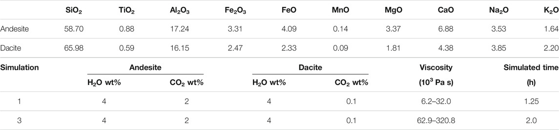
TABLE 1. Composition of magmas and list of simulations. For consistency with the corresponding 2D cases in (Garg et al., 2019), we keep the same simulations numbering here.

The numerical scheme and the stabilization terms employed for the solution of the set of Eqs 1–4 above, are reported in the Appendix.

3 Applications to Magma Mixing Dynamics

As discussed above, magmatic systems often consist of multiple heterogeneous magmas stored in a network of interconnected sills and dykes. Magma mixing is understood as one of many possible mechanisms for triggering an eruption (Sparks et al., 1977). Petrology and geochemistry analysis indicates that multiple intrusions of mafic to intermediate magma in more chemically evolved magmas stored at shallow depths may produce hybrid melts with zoned crystals. Sometimes the ejecta contain abundant inter-mingled hybrid magmas, suggesting efficient stirring and mingling in the reservoir as a result of replenishment and convection dynamics (Turner and Campbell, 1986; Petrelli et al., 2011; Longo et al., 2012a; Garg et al., 2019).

Arc volcanoes are known for their dominantly explosive character. Their erupted products span the so-called andesitic magmatic suite, ranging from basaltic andesite to rhyolite. The occurrence of repeated pre-eruptive mixing events involving andesitic and dacitic melts is often recognized in the discharged magmas [e.g., (Tamura et al., 2003; Shane et al., 2008; Conway et al., 2020)].

Here we employ the 3D physical model described above to study the physics of mixing between andesite and dacite magmas. We use these magmas because arc-volcanism emits mainly the andesitic suite of magmas. The objective is to study magma dynamics for this suite of magmas through numerical simulations and extract some geologically meaningful information. We remark that the model and numerical scheme employed here is applicable on any suite of magmas. In particular we model the convection dynamics emerging from a gravitationally unstable stratification of andesite and dacite magmas in a shallow reservoir. We refer to a set up that represents a 3D extension of the one employed in previous work (Garg et al., 2019), allowing us to also compare between 2D and 3D dynamics.

3.1 Simulation Setup

The computational domain represents a prolate ellipsoid with longer axis in the x direction (Figure 1). The centre of the ellipsoid is placed at 4.1 km depth. The lengths of the semi-axes in x, y, and z directions are 400, 100 and 100 m respectively. With respect to the 2D setup in (Garg et al., 2019), the third dimension added here (z-axis) is short enough to cause significant deviation from 2D conditions (approximated when the neglected dimension is much longer than the considered ones). We perform two simulations which correspond to run cases #1 and #3 in (Garg et al., 2019). For consistency with the corresponding 2D cases in (Garg et al., 2019), we keep the same numbering throughout in this work (Table 1). In the simulations, andesite at a temperature of 927°C is placed at the bottom of the domain, while the upper part is filled with dacite at a temperature of 876°C. A horizontal interface, separating the two magmas, is set at 4,150 m depth (Figure 1). The chemical composition of the two magmas and their volatile contents are reported in Table 1. The two cases differ for only magma viscosity, with case #1 corresponding to locally defined, space-time dependent viscosity computed as described above, and case #3 equal to case #1 with the viscosity arbitrarily multiplied by a factor 10 everywhere in space and time. The effects of varying the amount of volatile contents in the 2D setup were studied in (Garg et al., 2019). While such a viscosity increase may approximate the effect of non-reactive crystals, which affect viscosity much more than other properties including density, the aim here is mostly that of evaluating the 3D dynamics and comparing with the 2D case, over a range of viscosities thus of dynamic time scales; as well as that of evaluating the 3D code performance in terms of computational time and scalability. The initial pressure distribution is computed by considering the lithostatic load at the chamber roof (average rock density = 2,500 kg/m³) and a horizontally uniform magmastatic profile. The bottom panel of Figure 1 (red lines) displays the initial pressure and density profiles along the chamber axis. No-slip adiabatic conditions are employed at the chamber walls. The numerical scheme presented in the Appendix A is employed with 2.6 million linear tetrahedral elements. The side length of the computational elements ranges 1–4 m. The numerical integrals are computed with four Gauss quadrature points. The unstructured tetrahedral mesh results in uneven interface providing the initial perturbations that destabilize the interface between the two magma types. The simulations are run on an HP cluster system at INGV Pisa, composed of 432 Intel Xeon 2.3 GHz cores distributed over six nodes connected through a low latency 100 Gbps Infiniband network. Scaling tests reported below and involving up to thousands cores for a much shorter computational time are run instead on the supercomputing facilities at the Barcelona Supercomputing Center.

FIGURE 1

FIGURE 1. Simulations setup and profiles of pressure and density along chamber axis (x = 0, z = 0).

4 Results

We present the results of the numerical simulations by first analysing the 3D convection dynamics, then comparing with the 2D case in (Garg et al., 2019).

4.1 3D Dynamics

The 3D dynamics are illustrated here mostly through comparison between the two simulation cases 1 and 3 in Table 1, with the latter being identical to the former, except for the computed viscosity which is everywhere in space and time arbitrarily multiplied by a factor 10. We anticipate that as for the 2D case (Garg et al., 2019), the more viscous situation corresponds to slower convection dynamics, lower number of buoyant plumes of andesite-rich magma rising through the dacite, and finally lower mixing efficiency. Figure 2 illustrates well such differences. The figure shows the evolution of the isosurface corresponding to a mass fraction of andesite equal to 0.5 (which at time zero corresponds to the interface between the two magma types) for cases 1 and 3. The differences are striking: after 100 s case 1 shows a highly dynamic state with a complex structure made of several inter-digitized rising plumes interacting with each other and occupying the entire chamber; while at the same time, only minor perturbations appear on the interface initially separating the two dacitic and andesitic magmas. At a later time when the dynamics are well developed also for case 3, this case displays a much simpler overall structure with many less plumes, each one on average much bigger than for case 1. The 0.5 mass fraction isosurface for the more viscous case 3 is conserved within the chamber over a much longer time, and it is still visible after more than 2 h from start of the simulation. On the contrary, the same isosurface is completely lost in case 1 after only 5 min, as a consequence of much faster and more intense magma mixing for this lower viscosity case.

FIGURE 2

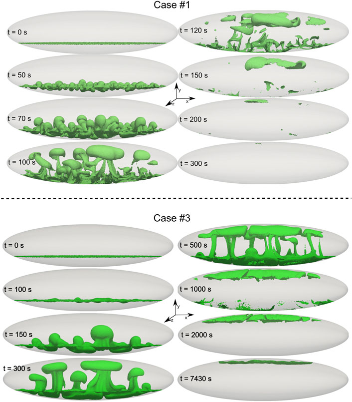
FIGURE 2. Temporal evolution of isosurfaces of mass fraction Y = 0.5.

Figure 3 highlights the differences in plume structure for the two cases, through a planar view of the interface at an early stage of its destabilization. The higher the viscosity (case 3), the lower the number density (and the larger the average size) of the rising plumes formed as a consequence of Rayleigh-Taylor Instabilities. Figure 4 shows instead the distribution of velocity in the uprising plumes, at the two times (90 and 250 s, respectively) at which the maximum velocity is attained for the two cases 1 and 3. That maximum velocity corresponds to 8.2 m/s in case 1, while it is only 3.5 m/s for the more viscous case 3.

FIGURE 3

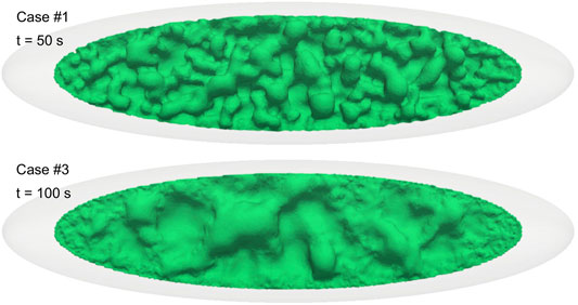
FIGURE 3. Plume structure looking at the interface from the top. The interface is depicted by isosurfaces of mass fraction Y = 0.5.

FIGURE 4

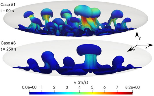
FIGURE 4. Velocity distribution of uprising plumes when the maximum value is reached.

Figure 5 illustrates the evolution of mixing throughout the computational domain. Case 1 corresponds to viscosity computed by model described in (Giordano et al., 2008) and case 3 is with tenfold increase in viscosity than case 1. Initially, for both cases 1 and 3 the computational nodes host either pure dacite or pure andesite. In both cases the less viscous, less abundant andesitic end-member quickly vanishes as a pure component (at the scale of the resolution of the present simulations, which is of order 1 m), whereas nearly pure dacite continues to be largely present in the system at the latest simulation times. Faster and more efficient mixing for case 1 is clearly visible as an earlier decrease of the maximum length of the compositional bars (that is, faster decrease of the number of nodes hosting pure dacite) as well as narrower compositional interval span inside the chamber at latest simulation times, when efficient convection is terminated in both cases (further illustrated below). For the more viscous case 3 the andesite can be seen to constitute at most about 50% of individual computational nodes, whereas for case 1 the maximum proportion of andesite in individual computational nodes at process end is only about 30%.

FIGURE 5

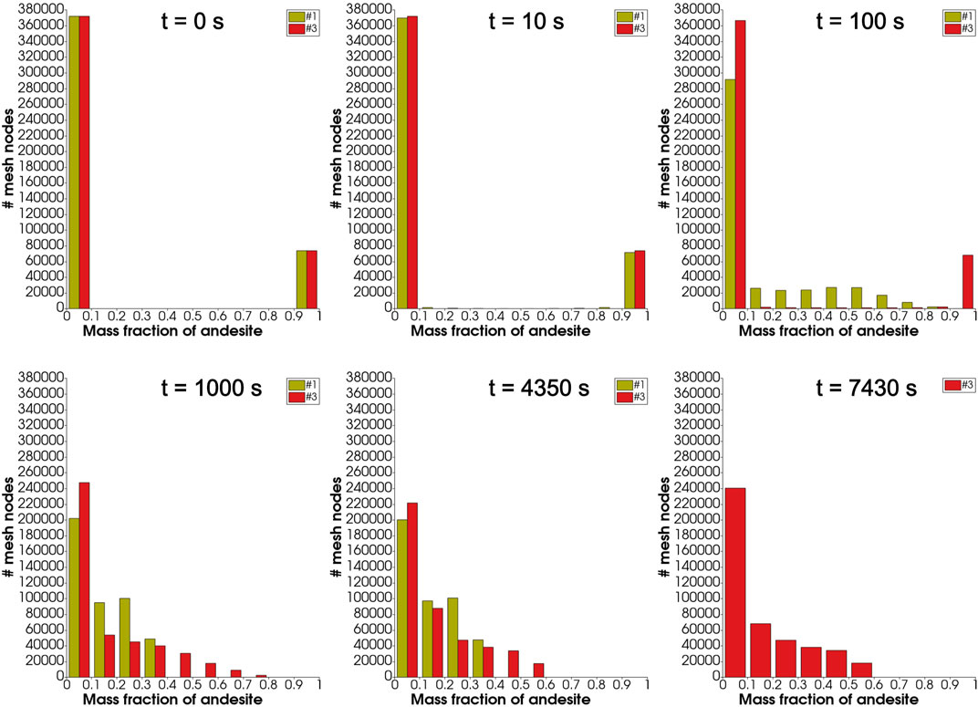
FIGURE 5. Distribution of composition across mesh nodes. Simulation case 1 was run up to 4,350 s. Therefore, at 7,430 s, only #3 is displayed.

In both cases 1 and 3 by the latest times, the system is decompressed throughout by 6 and 2 bars, respectively, and the density evolves from an initial step profile to a smooth one (Figure 1). For both simulation cases 1 and 3, pressure and temperature distributions along z = 0 and x = 0 planes is provided in the Supplementary Material. We also display the profiles of scaled temperature and composition along the chamber axis in the Supplementary Material.

4.2 Comparison Between 3D and 2D Simulation Results

As it is explained above, the present 3D simulation cases correspond to previous 2D simulations in (Garg et al., 2019), so to confidently explore the effects of 3D vs. 2D simulation setup. In particular, the numerical code and the physical and numerical setup in the 2D and 3D cases are the same, except for the specific aspects defining 2D vs. 3D simulated dynamics. The average length of computational elements across the initial compositional interface is of order 1 m in both cases, and the number of elements in the 2D cases and along domain-centered 2D slides in the 3D cases are of order 10⁵ in both cases.

One of the major results from the simulation of 2D magma convection dynamics was the achievement of a stable dynamic state characterized by separate convective regions effectively impeding further mechanical mixing (Garg et al., 2019). Figure 6 shows that such a major result is confirmed by 3D numerical simulations: dynamically stable, largely closed circulation patterns separating regions with different composition emerge, explaining the long-term maintenance of the heterogeneities at advanced times in Figure 5. In fact, the circulation patterns in Figure 6 give rise to a stable, dynamic layering inside the magma chamber (Figure 7). The details of the circulation patterns are not easy to compare, as those patterns are intimately three-dimensional for the 3D simulations, therefore, comparing a slice cut with the 2D case, e.g. as in Figures 8, 9 below, would not make any sense. Here we stress the overall first order agreement between the 2D and 3D simulation cases with respect to the major conclusion that magma chamber overturning and associated convection and mixing dynamics lead to the achievement of a stable dynamic state preserving compositional heterogeneities over the long term. We discuss in (Garg et al., 2019) some major consequences for the interpretation of compositional heterogeneities in magmas erupted during individual eruptions.

FIGURE 6

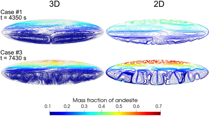
FIGURE 6. Streamline structure with composition colorbar.

FIGURE 7

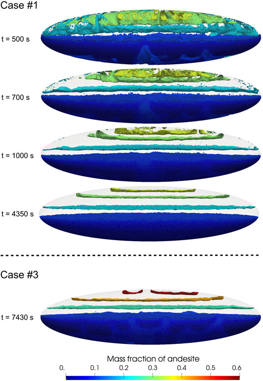
FIGURE 7. Temporal evolution of isosurfaces of mass fraction of andesite.

FIGURE 8

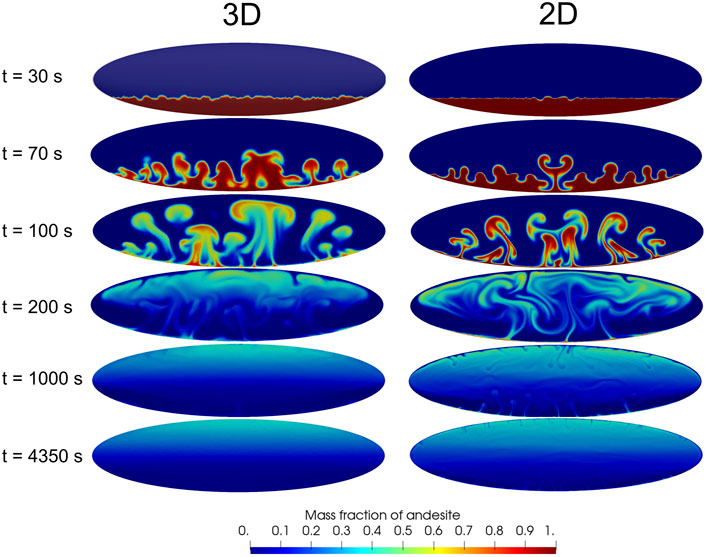
FIGURE 8. Comparison between 2D simulation and a vertical slice at z = 0 from the 3D simulation #1.

FIGURE 9

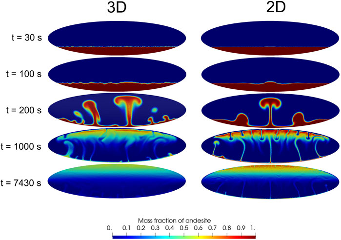
FIGURE 9. Comparison between 2D simulation and a vertical slice at z = 0 from the 3D simulation #3.

A more direct comparison between the simulated 2D and 3D dynamics is displayed in Figures 8, 9 for the simulation cases 1 and 3, respectively. For the 2D case each panel in the figures represents the entire computational domain, with the third neglected dimension (perpendicular to the sheet) assumed much longer than the two simulated ones so as to satisfy the 2D approximation. On the contrary, for the 3D case each panel reports a vertical slice cut across the center of the 3D computational domain, with the third dimension, simulated but not visible from the slice cut, being equal in size to the vertical dimension (Figure 1).

At first sight, the 3D and 2D dynamics in Figures 8, 9 appear quite similar, especially in light of the different evolutions characterizing the less and more viscous cases, respectively, one and 3. That may appear surprising, considering the small length of the third chamber dimension in the present 3D simulations. However, such qualitative similarities are consistent with previous findings, e.g., (Young et al., 2001; Cabot, 2006) (although those authors investigate high-Re incompressible flows), and as for those cases, we show here that the differences are also relevant.

The comparison shows that the interface destabilization time in the two 3D and 2D cases is very similar [while it is significantly influenced, as any other aspect of the overall dynamics, by magma viscosity. The role of viscosity—and of volatile contents—is however described in (Garg et al., 2019), and it is only marginally considered here]. However, the 3D geometry of the interface appears to result in more complex perturbation structure comprising a broad range of scales, compared to the geometrically much simpler 2D perturbations. At later times such a richer 3D structure is visible as a much less symmetric geometry of the rising plumes, and more widespread plume size range. The plumes in the 3D cases also appear to rise faster, and are more mixed than for the 2D cases. That is well evident at time 100 s for case 1 (Figure 8) or time 200 s for case 2 (Figure 9): the 2D plumes maintain a much larger proportion of nearly pure andesite (dark red), which is instead much less represented (Figure 9), or practically absent (Figure 8), in the 3D cases at the same time. At the latest simulation times corresponding to achievement of a stable dynamic stratification as discussed above, the more viscous case in Figure 9 shows that andesite-rich (70–80 wt%) magma concentrates close to magma chamber top in the 2D case, whereas only $<$ 60 wt% andesitic magma occupies the same chamber region in the 3D case.

The faster, more efficient mixing dynamics found for the 3D case are best highlighted in Figure 10. Here, to establish a measure of mixing, we refer to progressive reduction of the overall compositional heterogeneity inside the chamber. As a quantitative measure of such heterogeneity we compute the standard deviation (σ) of the mass fraction of andesite in the overall computational domain. For any time we first determine the mean value of the composition in the entire domain, then use that value to compute (σ), which measures the extent of dispersion of the composition around its mean value. The larger the value of (σ), the lower the extent of mixing:

$\sigma =\sqrt{\frac{1}{N}\sum _{i=1}^N{\left(x_{i,and}-{\bar{x}}_{and}\right)}^2}(9)$

where N is the total number of nodes in the computational domain, x is mass fraction, and the horizontal bar indicates the mean value over the entire computational domain.

FIGURE 10

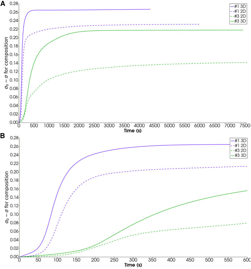
FIGURE 10. Panel (A): Evolution of overall compositional heterogeneities. σ is overall compositional standard deviation and σ₀ is the same quantity at time zero. Panel (B): Zoom view of first 600 s.

The computed evolutions of σ in Figure 10 for the 2D and 3D simulations evidence the different stages of the overturning process (Garg et al., 2019), starting in all cases with a low slope section corresponding to the initial phase 1 of development of the Rayleigh-Taylor instability, followed by a high slope section corresponding to highly efficient mixing during the convective phase of plume rise and vortex formation (phase 2), and terminating with an essentially flat section (phase 3) when the final stable dynamic state described above, preventing significant further mixing, is achieved. Faster development of the Rayleigh-Taylor instability and transition to phase 2 (efficient plume rise) is highlighted in the zoom view of Figure 10B. Similarly, faster overall dynamics and more efficient mixing for the 3D case translate in earlier achievement of the flat section corresponding to phase 3. Note that for the high-viscosity case 3, the 2D simulation never attains a completely flat section, indicating that some mixing continues to be effective up to the last simulated time $>$ 2 h. That suggests that constraining the magma circulation patterns over a 2D plane (or better, assuming zero gradient of any flow variable including velocity along the neglected dimension as it is implicit in 2D simulations) may cause the flow streamlines to distort to an extent sufficient to break the closed circulation patterns in Figure 6, resulting in further mixing not seen at such late times from the 3D simulations. Finally, and mostly relevant, the final extent of homogenization (that is, the overall change in σ) is significantly larger for the 3D simulation cases, reflecting enhanced convection and mixing efficiency with respect to the 2D case. The difference is important, amounting to 18% of the total σ change computed from the 2D simulation for case 1, and as large as 55% of that change for case 3. Therefore, not only mixing and homogenization in the magma chamber are significantly enhanced when considering the flow dynamics in a more realistic 3D environment; also, the extent of such enhancement depends substantially on the specific conditions. While the less viscous case 1 leads to more homogenization, the extent of change when moving from 2D to 3D turns out to be larger for the more viscous case 3. In other words, it seems plausible, based on our first 3D simulations and comparison with the corresponding 2D cases, to suggest that the errors and approximations introduced by neglecting more realistic 3D dynamics may vary substantially depending on the conditions considered, and may increase in relevance with increasing magma viscosity.

5 Code Performance

As we mention above, the 3D simulation results presented above make use of 2.6 million tethrahedral elements in order to resolve the 3D Rayleigh-Taylor flow structure determined by the adopted initial unstable configuration. Figure 11 shows a zoom view of one isosurface distribution from Figure 2. In particular, superposition of the computational mesh illustrates well the resolution level achieved, and the kind of details that are resolved.

FIGURE 11

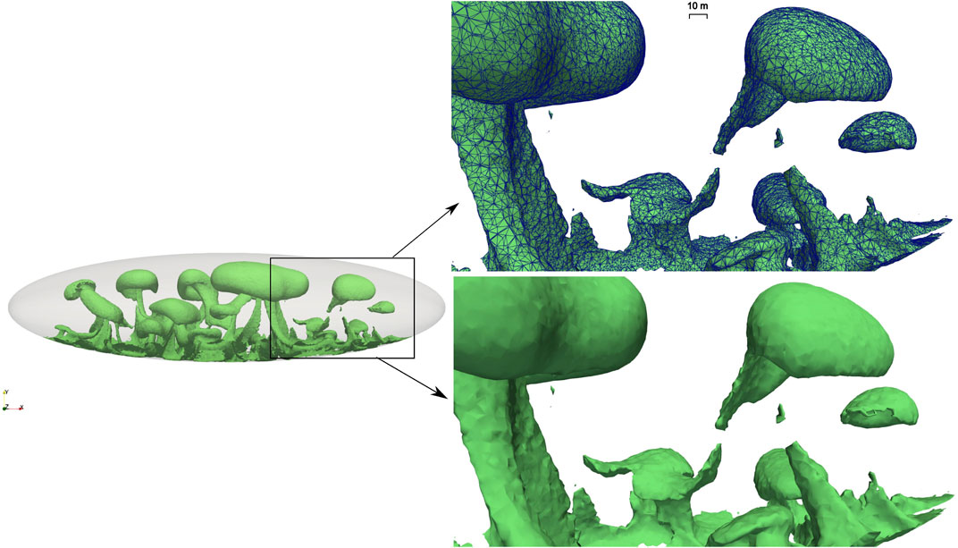
FIGURE 11. Zoom view of the computational mesh and isosurfaces Y = 0.5 at t = 100 s for case #1.

To check the parallel performance of GALES, we conduct a strong scaling test which is widely used to check the ability of a software to deliver results in less time when the amount of resources is increased. The parallel performance is quantified by comparing the actual speedup with the ideal speedup for a given set of processors. The actual speedup and the ideal speedup are defined as

$\text{Actual\hspace{0.17em}speedup}=\frac{t_r}{t_N}r<N(10)$

$\text{Ideal\hspace{0.17em}speedup}=\frac{N}{r}(11)$

where t_r and t_N are the computational times taken by r processors and N processors, respectively. Parallel efficiency is computed as the ratio of the actual speedup and the ideal speedup for a given number of processors:

$\text{Efficiency}=\frac{t_r}{t_N}.\frac{r}{N}(12)$

An ideal scalable software should result in a linear speedup. However, this is hardly achieved in real situations. For a given mesh the parallel efficiency decreases as we increase the number of processors, mostly as a consequence of increased time spent in communication among processors. The scaling tests are performed on the Marenostrum supercomputer at the Barcelona Supercomputing Centre (BSC) (https://www.bsc.es/marenostrum/marenostrum/technical-information) within the project GALES-3D (2010PA5625) in the frame of a PRACE preparatory access A (https://prace-ri.eu/).

The scaling tests were run on three different meshes with progressively increasing size. The mesh models are listed in Table 2. The simulations use the same setup as described in Section 3.1. The adopted numerical methods and the parallelization strategy employed are illustrated in detail in Appendixes A,B. Here we only recall the monolithic approach to solve the linearized system of equations describing the space-time system dynamics, which is effective in reducing data transfer in parallel computing implementations (Dowd and Charles, 2010).

TABLE 2

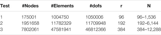
TABLE 2. Mesh models for strong scaling test.

Figure 12 shows the strong scaling results for each test case. The left panels in the figure display the time taken by the assembly procedure, the linear solver and the total time. We report here the average time taken for a non-linear iteration over 10 time steps (the observed standard deviation being 2 × 10^–2 s). The right panels in the figure plot the speedup and the efficiency as a function of number of cores.

FIGURE 12

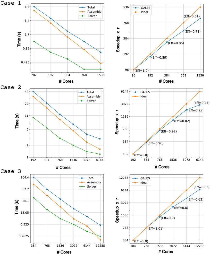
FIGURE 12. Strong scaling results for test cases in Table 2.

Overall, the scaling behavior of GALES is quite satisfactory in the explored range of computational elements and cores (a parallel efficiency of 0.6 or greater is taken here as satisfactory). The left panels in Figure 12 show that most of the computational time is spent in the assembly of the linearized system of equations. The solution time is only a fraction of the assembly time, increasing in relevance with increasing number of cores thus (right panels) with decreasing parallel efficiency. The total computational time decays nearly linearly (in the log scale of the figures) with increasing number of cores, and the parallel efficiency (right panels) is seen to decrease below satisfactory only for the largest number of cores employed for each different mesh size.

Parallel performance primarily depends on load balancing and inter-processor communication. Our linear solvers are distributed and use peer-to-peer communication to solve the system. Table 3 displays the partition statistics for test case 3 in Table 2, and illustrates well the reasons and conditions under which the parallel efficiency becomes less than satisfactory. Specifically, we display the average number of elements on a processor and the average percentage of inter-processor boundary nodes, computed from the load balanced partitions generated by the Metis software (see the Appendix B for further details). Load balance when increasing the computational resources reduces the overall execution time. However, by increasing the number of processors the percentage of boundary nodes lying at inter-processor boundaries also increases, implying that the processors need to communicate more data. This translates into increased communication time and works towards decreased parallel efficiency. In other words, for any specific problem there is an optimal balance between decreasing load per core and increasing core inter-communication when increasing the overall computational resources. The results in Figure 12 show that for GALES, and in the range of the strong scaling exercise described here, a one order of magnitude decrease in total computational time is allowed before such a balancing condition is achieved.

TABLE 3

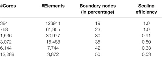
TABLE 3. Partitioning statistics for test case 3 in Table 2. The second column reports the average number of elements per core. The third column reports the average percentage of nodes lying on inter-processor boundaries.

6 Discussion and Conclusion

In this paper we present a 3D parallel code for computing compressible to incompressible multi-component magma dynamics, compare numerical simulations of 3D vs. 2D dynamics for a simple test case represented by the development of Rayleigh-Taylor instability in a stratified, idealized magma chamber, and illustrate code performance by analyzing the results of a strong scaling test involving up to nearly 50 million computational elements and up to $>$12,000 computational cores. The computational speedup is close to ideal and above satisfactory levels as long as the element/core ratio is sufficiently large so as to limit boundary nodes to less than half total nodes. The demonstrated parallel efficiency is such as to guarantee efficient use of HPC resources in 3D applications to more realistic magmatic configurations including geometrically complex multiple chamber, dike and conduit systems, likely requiring a number of computational elements exceeding the maximum employed here. Recent extension of GALES to include fluid-structure interaction and coupling with solid elasto-dynamics (Garg et al., 2021) further extends the accessible computational domains requiring exploration of the potential towards exascale computing (e.g., as in the ChEESE European Center of Excellence, www.cheese-coe.eu).

The numerical simulations performed here, designed to compare with previous 2D simulations, illustrate the 3D dynamics of magma chamber overturning due to gravitationally unstable initial conditions and development and evolution of Rayleigh-Taylor instability. The numerical results illustrate to a high resolution level the 3D dynamics of development and growth of the instability, the formation and reciprocal interaction of buoyant plumes of magma, the complexities of the associated vorticity patterns and associated magma mixing, and the evolution towards a stable dynamic state preserving compositional heterogeneities and resulting in a dynamic layering of the magma chamber.

Remarkably, the much simpler 2D simulation approach is found to reproduce the more realistic 3D dynamics on a zero/first-order level, showing similar overall dynamics occurring over comparable time scales, and similar overall effects due to increased magma viscosity. On a more quantitative level, the 3D dynamics show however important differences, and in particular they produce faster plumes leading to more efficient magma mixing than for the corresponding 2D approximation. These results are in general consistent with those from the engineering literature (Young et al., 2001; Cabot, 2006) where similar overall qualitative consistency but important quantitative differences between 2D and 3D simulations are evidenced, although for high Re incompressible flows. In particular, our results suggest that the extent of approximation introduced by the 2D simplification may depend on the specific conditions, and may be smaller for low viscosity conditions. That could be relevant in light of the substantial computational efforts required by the solution of 3D dynamics, and we deserve to evaluate it further, e.g., for more complex geometrical systems over a range of magmatic compositions.

Data Availability Statement

The raw data supporting the conclusion of this article will be made available by the authors, without undue reservation.

Author Contributions

DG and PP designed the study, analysed and discussed the results, and wrote the article, DG carried out the numerical simulations and postprocessed the results.

Conflict of Interest

The authors declare that the research was conducted in the absence of any commercial or financial relationships that could be construed as a potential conflict of interest.

Publisher’s Note

All claims expressed in this article are solely those of the authors and do not necessarily represent those of their affiliated organizations, or those of the publisher, the editors and the reviewers. Any product that may be evaluated in this article, or claim that may be made by its manufacturer, is not guaranteed or endorsed by the publisher.

Acknowledgments

We gratefully acknowledge the reviewers for their comments, which improve the quality of the manuscript. We acknowledge that the results on the code performance have been achieved using the PRACE Research Infrastructure resource MareNostrum based in Spain at Barcelona Supercomputing Centre (BSC). One of us (D.G.) was supported by an EPOS-IT grant.

Supplementary Material

The Supplementary Material for this article can be found online at: https://www.frontiersin.org/articles/10.3389/feart.2021.760773/full#supplementary-material

References

Asanovic, K., Bodik, R., Gebis, J., Husbands, P., Keutzer, K., Shalf, J., et al. (2006). Technical report. Berkeley: EECS Department, University of California. The Landscape of Parallel Computing Research: A View from berkeley.

Google Scholar

Bachmann, O., and Bergantz, G. W. (2003). Rejuvenation of the Fish canyon Magma Body: A Window into the Evolution of Large-Volume Silicic Magma Systems. Geol. 31 (9), 789–792. doi:10.1130/g19764.1

CrossRef Full Text | Google Scholar

Bagagli, M., Montagna, C. P., Papale, P., and Longo, A. (2017). Signature of Magmatic Processes in Strainmeter Records at Campi Flegrei (italy). Geophys. Res. Lett. 44, 718–725. doi:10.1002/2016gl071875

CrossRef Full Text | Google Scholar

Bavier, E., Hoemmen, M., Rajamanickam, S., and Thornquist, H. (2012). Amesos2 and Belos: Direct and Iterative Solvers for Large Sparse Linear Systems. Scientific Programming 20 (3), 241–255. doi:10.1155/2012/243875

CrossRef Full Text | Google Scholar

Bazilevs, Y., Calo, V., Cottrell, J. A., Hughes, T., Reali, A., Scovazzi, G., et al. (2007). Variational Multiscale Residual-Based Turbulence Modeling for Large Eddy Simulation of Incompressible Flows. CMAME 197 (1), 173–201. doi:10.1016/j.cma.2007.07.016

CrossRef Full Text | Google Scholar

Bergantz, G. W. (2000). On the Dynamics of Magma Mixing by Reintrusion: Implications for Pluton Assembly Processes. J. Struct. Geology 22 (22), 1297–1309. doi:10.1016/s0191-8141(00)00053-5

CrossRef Full Text | Google Scholar

Bergantz, G. W., Schleicher, J. M., and Burgisser, A. (2015). Open-system Dynamics and Mixing in Magma Mushes. Nat. Geosci. 8, 793–796. doi:10.1038/ngeo2534

CrossRef Full Text | Google Scholar

Blundy, J. D., and Annen, C. J. (2016). Crustal Magmatic Systems from the Perspective of Heat Transfer. Elements 12 (2), 115–120. doi:10.2113/gselements.12.2.115

CrossRef Full Text | Google Scholar

Burnham, C. W., Holloway, J. R., and Davis, N. F. (1969). Thermodynamic Properties of Water to 1,000° C and 10,000 Bars. Geol. Soc. America Spec. Pap. 132, 1–96. doi:10.1130/spe132-p1

CrossRef Full Text | Google Scholar

Cabot, W. (2006). Comparison of Two- and Three-Dimensional Simulations of Miscible Rayleigh-taylor Instability. Phys. Fluids 18, 1–9. doi:10.1063/1.2191856

CrossRef Full Text | Google Scholar

Campbell, I. H., and Turner, J. S. (1986). The Influence of Viscosity on Fountains in Magma chambers. J. Petrology 27, 1–30. doi:10.1093/petrology/27.1.1

CrossRef Full Text | Google Scholar

Caricchi, L., Burlini, L., Ulmer, P., Gerya, T., Vassalli, M., and Papale, P. (2007). Non-newtonian Rheology of crystal-bearing Magmas and Implications for Magma Ascent Dynamics. Earth Planet. Sci. Lett. 264, 402–419. doi:10.1016/j.epsl.2007.09.032

CrossRef Full Text | Google Scholar

Carrara, A. (2019). Numerical Modeling of the Physical Processes Causing the Reawakening of a Magmatic Chamber and of the Associated Geophysical Signals Theses Grenoble: Université Grenoble Alpes.

Google Scholar

Cashman, C. (2000). Encyclopedia of Volcanoes. Academic Press.

Google Scholar

Cassidy, M., Manga, M., Cashman, K., and Bachmann, O. (2018). Controls on Explosive-Effusive Volcanic Eruption Styles. Nat. Commun. 9 (2839), 1–16. doi:10.1038/s41467-018-05293-3

PubMed Abstract | CrossRef Full Text | Google Scholar

Conway, C. E., Chamberlain, K. J., Harigane, Y., Morgan, D. J., and Wilson, C. J. N. (2020). Rapid Assembly of High-Mg Andesites and Dacites by Magma Mixing at a continental Arc Stratovolcano. Geology 48, 1033–1037. doi:10.1130/g47614.1

CrossRef Full Text | Google Scholar

Couch, S., Sparks, R. S. J., and Carroll, M. R. (2001). Mineral Disequilibrium in Lavas Explained by Convective Self-Mixing in Open Magma chambers. Nature 411, 1037–1039. doi:10.1038/35082540

PubMed Abstract | CrossRef Full Text | Google Scholar

De Campos, C. P., Perugini, D., Ertel-Ingrisch, W., Dingwell, D. B., and Poli, G. (2011). Enhancement of Magma Mixing Efficiency by Chaotic Dynamics: an Experimental Study. Contrib. Mineral. Petrol. 161, 863–881. doi:10.1007/s00410-010-0569-0

CrossRef Full Text | Google Scholar

DePaolo, D. J. (1981). Trace Element and Isotopic Effects of Combined Wallrock Assimilation and Fractional Crystallization. Earth Planet. Sci. Lett. 53 (2), 189–202. doi:10.1016/0012-821x(81)90153-9

CrossRef Full Text | Google Scholar

Dowd, K., and Charles, S. (2010). High Performance Computing. Texas: Rice University.

Google Scholar

Edmonds, M., and Wallace, P. J. (2017). Volatiles and Exsolved Vapor in Volcanic Systems. Elements 13 (1), 29–34. doi:10.2113/gselements.13.1.29

CrossRef Full Text | Google Scholar

Eichelberger, J. (2020). Distribution and Transport of thermal Energy within Magma–Hydrothermal Systems. Geosciences 10, 1–26. doi:10.3390/geosciences10060212

PubMed Abstract | CrossRef Full Text | Google Scholar

Flanagan, J., Davies, G. H., Boy, F., and Doneddu, D. (2020). A Review of a Distributed High Performance Computing Implementation. J. Inf. Technology Case Appl. Res. 22 (3), 142–158. doi:10.1080/15228053.2020.1812803

CrossRef Full Text | Google Scholar

Folch, A., and Marti, J. (1998). The Generation of Overpressure in Felsic Magma chambers by Replenishment. Earth Planet. Sci. Lett. 163 (1), 301–314. doi:10.1016/s0012-821x(98)00196-4

CrossRef Full Text | Google Scholar

Franco, R., and Rafael Saavedra, G. Z. (2006). A Stabilized Finite Element Method Based on Sgs Models for Compressible Flows. Computer Methods Appl. Mech. Eng. 196 (1), 652–664.

Google Scholar

Garg, D., Papale, P., Colucci, S., and Longo, A. (2019). Long-lived Compositional Heterogeneities in Magma chambers, and Implications for Volcanic hazard. Sci. Rep. 9 (3321), 1–13. doi:10.1038/s41598-019-40160-1

PubMed Abstract | CrossRef Full Text | Google Scholar

Garg, D., Longo, A., and Papale, P. (2018a). Computation of Compressible and Incompressible Flows with a Space-Time Stabilized Finite Element Method. Comput. Mathematics Appl. 75, 4272–4285. doi:10.1016/j.camwa.2018.03.028

CrossRef Full Text | Google Scholar

Garg, D., Longo, A., and Papale, P. (2018b). Modeling Free Surface Flows Using Stabilized Finite Element Method. Math. Probl. Eng. 2018 (6154251), 1–9. doi:10.1155/2018/6154251

CrossRef Full Text | Google Scholar

Garg, D., Papale, P., and Longo, A. (2021). A Partitioned Solver for Compressible/incompressible Fluid Flow and Light Structure. Comput. Mathematics Appl. 100, 182–195. doi:10.1016/j.camwa.2021.09.005

CrossRef Full Text | Google Scholar

Giordano, D., Russell, J. K., and Dingwell, D. B. (2008). Viscosity of Magmatic Liquids: a Model. Earth Planet. Sci. Lett. 271, 123–134. doi:10.1016/j.epsl.2008.03.038

CrossRef Full Text | Google Scholar

Gottlieb, A. (1989). Highly Parallel Computing. Redwood City, CA: Benjamin-Cummings Publishing Co., Inc..

Google Scholar

Gottsmann, J., De Angelis, S., Fournier, N., Van Camp, M., Sacks, S., Linde, A., et al. (2011). On the Geophysical Fingerprint of Vulcanian Explosions. Earth Planet. Sci. Lett. 306 (1), 98–104. doi:10.1016/j.epsl.2011.03.035

CrossRef Full Text | Google Scholar

Gudmundsson, A. (2011). Deflection of Dykes into Sills at Discontinuities and Magma-Chamber Formation. Tectonophysics 500 (1), 50–64. doi:10.1016/j.tecto.2009.10.015

CrossRef Full Text | Google Scholar

Gudmundsson, A. (1995). Infrastructure and Mechanics of Volcanic Systems in iceland. J. Volcanology Geothermal Res. 64 (1), 1–22. doi:10.1016/0377-0273(95)92782-q

CrossRef Full Text | Google Scholar

Gudmundsson, A. (2012). Magma chambers: Formation, Local Stresses, Excess Pressures, and Compartments. J. Volcanology Geothermal Res. 237-238, 19–41. doi:10.1016/j.jvolgeores.2012.05.015

CrossRef Full Text | Google Scholar

Gutiérrez, F., and Miguel, A. (2010). Parada. Numerical Modeling of Time-dependent Fluid Dynamics and Differentiation of a Shallow Basaltic Magma Chamber. J. Petrology 51 (3), 731–762.

Google Scholar

Hauke, G., and Hughes, T. J. R. (1998). A Comparative Study of Different Sets of Variables for Solving Compressible and Incompressible Flows. CMAME 153 (1–2), 1–44. doi:10.1016/s0045-7825(97)00043-1

CrossRef Full Text | Google Scholar

Hauke, G., and Hughes, T. J. R. (1994). A Unified Approach to Compressible and Incompressible Flows. CMAME 113 (3), 389–395. doi:10.1016/0045-7825(94)90055-8

CrossRef Full Text | Google Scholar

Hauke, G. (2001). Simple Stabilizing Matrices for the Computation of Compressible Flows in Primitive Variables. CMAME 190 (51–52), 6881–6893. doi:10.1016/s0045-7825(01)00267-5

CrossRef Full Text | Google Scholar

Hughes, T. J. R., Feijoo, G., Mazzei, L., and Quincy, J. B. (1998). The Variational Multiscale Method—A Paradigm for Computational Mechanics. Computer Methods Appl. Mech. Eng. 166 (1), 3–24. doi:10.1016/s0045-7825(98)00079-6

CrossRef Full Text | Google Scholar

Hughes, T. J. R. (1995). Multiscale Phenomena: Green’s Functions, the Dirichlet-To-Neumann Formulation, Subgrid Scale Models, Bubbles and the Origins of Stabilized Methods. Computer Methods Appl. Mech. Eng. 127 (1), 387–401. doi:10.1016/0045-7825(95)00844-9

CrossRef Full Text | Google Scholar

Huppert, H. E., Sparks, R. S. J., Whitehead, J. A., and Hallworth, M. A. (1986). Replenishment of Magma chambers by Light Inputs. J. Geophys. Res. 91, 6113–6122. doi:10.1029/jb091ib06p06113

CrossRef Full Text | Google Scholar

Ishii, M., and Zuber, N. (1979). Drag Coefficient and Relative Velocity in Bubbly, Droplet or Particulate Flows. Aiche J. 25, 843–855. doi:10.1002/aic.690250513

CrossRef Full Text | Google Scholar

Jellinek, A. M., and Kerr, R. C. (1999). Mixing and Compositional Stratification Produced by Natural Convection: 2. Applications to the Differentiation of Basaltic and Silicic Magma chambers and Komatiite Lava Flows. J. Geophys. Res. 104, 7203–7218. doi:10.1029/1998jb900117

CrossRef Full Text | Google Scholar

Karlstrom, L., Dufek, J., and Manga, M. (2010). Magma Chamber Stability in Arc and continental Crust. J. Volcanology Geothermal Res. 190 (3), 249–270. doi:10.1016/j.jvolgeores.2009.10.003

CrossRef Full Text | Google Scholar

Karypis, G., and Kumar, V. (1999). A Fast and High Quality Multilevel Scheme for Partitioning Irregular Graphs. SIAM J. Scientific Comput. 20 (1), 359–392.

Google Scholar

Lange, R. A. (1994). Chapter 9. The Effect of H₂0, CO₂ and F on the Density and Viscosity of Silicate Melts. Rev. Mineralogy 30, 331–370. doi:10.1515/9781501509674-015

CrossRef Full Text | Google Scholar

Laumonier, M., Scaillet, B., Pichavant, M., Champallier, R., Andujar, J., and Arbaret, L. (2014). On the Conditions of Magma Mixing and its Bearing on Andesite Production in the Crust. Nat. Commun. 5 (1–12), 5607. doi:10.1038/ncomms6607

PubMed Abstract | CrossRef Full Text | Google Scholar

Lieto, B. D., Romano, P., Scarpa, R., and Linde, A. T. (2020). Strain Signals before and during Paroxysmal Activity at Stromboli Volcano, Italy. Geophys. Res. Lett. 47, 1–9. doi:10.1029/2020gl088521

CrossRef Full Text | Google Scholar

Longo, A., Barsanti, M., Cassioli, A., and Papale, P. (2012). A Finite Element Galerkin/Least-Squares Method for Computation of Multicomponent Compressible-Incompressible Flows. Comput. Fluids 67, 57–71. doi:10.1016/j.compfluid.2012.07.008

CrossRef Full Text | Google Scholar

Longo, A., Papale, P., Vassalli, M., Saccorotti, G., Montagna, C. P., Cassioli, A., et al. (2012). Magma Convection and Mixing Dynamics as a Source of Ultra-long-period Oscillations. Bull. Volcanol. 74, 873–880. doi:10.1007/s00445-011-0570-0

CrossRef Full Text | Google Scholar

Michioka, H., and Sumita, I. (2005). Rayleigh-taylor Instability of a Particle Packed Viscous Fluid: Implications for a Solidifying Magma. Geophys. Res. Lett. 32 (3), 1–4. doi:10.1029/2004gl021827

CrossRef Full Text | Google Scholar

Morgavi, D., Petrelli, M., Vetere, F. P., González-García, D., and Perugini, D. (2015). High-temperature Apparatus for Chaotic Mixing of Natural Silicate Melts. Rev. Scientific Instr. 86, 105108. doi:10.1063/1.4932610

CrossRef Full Text | Google Scholar

Pal, R. (2003). Rheological Behavior of Bubble-Bearing Magmas. Earth Planet. Sci. Lett. 207 (1), 165–179. doi:10.1016/s0012-821x(02)01104-4

CrossRef Full Text | Google Scholar

Papale, P., Montagna, C. P., and Longo, A. (2017). Pressure Evolution in Shallow Magma chambers upon Buoyancy-Driven Replenishment. Geochem. Geophys. Geosyst. 18, 1214–1224. doi:10.1002/2016gc006731

CrossRef Full Text | Google Scholar

Papale, P., Moretti, R., and Barbato, D. (2006). The Compositional Dependence of the Saturation Surface of H₂O+CO₂ Fluids in Silicate Melts. Chem. Geology 229, 78–95. doi:10.1016/j.chemgeo.2006.01.013

CrossRef Full Text | Google Scholar

Perugini, D., De Campos, C. P., Petrelli, M., and Dingwell, D. B. (2015). Concentration Variance Decay during Magma Mixing: a Volcanic Chronometer. Sci. Rep. 5 (14225), 1–10. doi:10.1038/srep14225

CrossRef Full Text | Google Scholar

Petrelli, M., Perugini, D., and Poli, G. (2011). Transition to Chaos and Implications for Time-Scales of Magma Hybridization during Mixing Processes in Magma Chambers. Lithos 125 (1), 211–220. doi:10.1016/j.lithos.2011.02.007

CrossRef Full Text | Google Scholar

Rispoli, F., Delibra, G., Venturini, P., Corsini, A., Saavedra, R., and Tezduyar, T. E. (2015). Particle Tracking and Particle-Shock Interaction in Compressible-Flow Computations with the V-SGS Stabilization and Y Z β Shock-Capturing. Comput. Mech. 55, 1201–1209. doi:10.1007/s00466-015-1160-3

CrossRef Full Text | Google Scholar

Sato, E., and Sato, H. (2009). Study of Effect of Magma Pocket on Mixing of Two Magmas with Different Viscosities and Densities by Analogue Experiments. J. Volcanology Geothermal Res. 181 (1–2), 115–123. doi:10.1016/j.jvolgeores.2009.01.005

CrossRef Full Text | Google Scholar

Schleicher, J. M., Bergantz, G. W., Breidenthal, R. E., and Burgisser, A. (2016). Time Scales of crystal Mixing in Magma Mushes. Geophys. Res. Lett. 43, 1543–1550. doi:10.1002/2015gl067372

CrossRef Full Text | Google Scholar

Semenov, A. N., and Polyansky, O. P. (2017). Numerical Modeling of the Mechanisms of Magma Mingling and Mixing: A Case Study of the Formation of Complex Intrusions. Russ. Geology Geophys. 58, 1317–1332. doi:10.1016/j.rgg.2017.11.001

CrossRef Full Text | Google Scholar

Shakib, F., Hughes, T., and Johan, Z. (1991). A New Finite Element Formulation for Computational Fluid Dynamics: X. The Compressible Euler and Navier-Stokes Equations. CMAME 89 (1–3), 141–219. doi:10.1016/0045-7825(91)90041-4

CrossRef Full Text | Google Scholar

Shane, P., Doyle, L. R., and Nairn, I. A. (2008). Heterogeneous Andesite-Dacite Ejecta in 26-16.6 Ka Pyroclastic Deposits of Tongariro Volcano, New Zealand: the Product of Multiple Magma-Mixing Events. Bull. Volcanol. 70, 517–536. doi:10.1007/s00445-007-0152-3

CrossRef Full Text | Google Scholar

Sides, I., Edmonds, M., Maclennan, J., Houghton, B. F., Swanson, D. A., Maclnnis, M. J., et al. (2014). Magma Mixing and High Fountaining during the 1959 Kīlauea Iki Eruption, Hawai‘i. Earth Planet. Sci. Lett. 400, 102–112. doi:10.1016/j.epsl.2014.05.024

CrossRef Full Text | Google Scholar

Sparks, R. S. J., and Cashman, K. V. (2017). Dynamic Magma Systems: Implications for Forecasting Volcanic Activity. Elements 13, 35–40. doi:10.2113/gselements.13.1.35

CrossRef Full Text | Google Scholar

Sparks, R. S. J., and Huppert, H. E. (1984). Density Changes during the Fractional Crystallization of Basaltic Magmas: Fluid Dynamic Implications. Contr. Mineral. Petrol. 85, 300–309. doi:10.1007/bf00378108

CrossRef Full Text | Google Scholar

Sparks, S. R. J., Sigurdsson, H., and Wilson, L. (1977). Magma Mixing: a Mechanism for Triggering Acid Explosive Eruptions. Nature 267, 315–318. doi:10.1038/267315a0

CrossRef Full Text | Google Scholar

Sundermeyer, C., Gätjen, J., Weimann, L., and Worner, G. (2020). Timescales from Magma Mixing to Eruption in Alkaline Volcanism in the Eifel Volcanic fields, Western germany. Contrib. Mineral. Petrol. 175, 1–23. doi:10.1007/s00410-020-01715-y

CrossRef Full Text | Google Scholar

Tamura, Y., Yuhara, M., Ishii, T., Irino, N., and Shukuno, H. (2003). Andesites and Dacites from Daisen Volcano, Japan: Partial-To-Total Remelting of an Andesite Magma Body. J. Petrology 44 (12), 2243–2260. doi:10.1093/petrology/egg076

CrossRef Full Text | Google Scholar

Tezduyar, T. E., and Senga, M. (2006). Stabilization and Shock-Capturing Parameters in Supg Formulation of Compressible Flows. Computer Methods Appl. Mech. Eng. 195 (13), 1621–1632. doi:10.1016/j.cma.2005.05.032

CrossRef Full Text | Google Scholar

The Belos Project Team (2021). The BELOS Project Website.

Google Scholar

The Epetra Project Team (2021). The EPETRA Project Website.

Google Scholar

The Trilinos Project Team (2021). The Trilinos Project Website.

Google Scholar

Tomiya, A., Miyagi, I., Saito, G., and Geshi, N. (2013). Short Time Scales of Magma-Mixing Processes Prior to the 2011 Eruption of Shinmoedake Volcano, Kirishima Volcanic Group, Japan. Bull. Volcanol. 75, 1–19. doi:10.1007/s00445-013-0750-1

CrossRef Full Text | Google Scholar

Turner, J. S., and Campbell, I. H. (1986). Convection and Mixing in Magma chambers. Earth-Science Rev. 23 (4), 255–352. doi:10.1016/0012-8252(86)90015-2

CrossRef Full Text | Google Scholar

Vollaire, C., Nicolas, L., and Nicolas, A. (1998). Parallel Computing for the Finite Element Method. Eur. Phys. J. Appl. Phys. 1, 305–314.

CrossRef Full Text | Google Scholar

Xu, F., Moutsanidis, G., Kamensky, D., Hsu, M.-C., Murugan, M., Ghoshal, A., et al. (2017). Compressible Flows on Moving Domains: Stabilized Methods, Weakly Enforced Essential Boundary Conditions, Sliding Interfaces, and Application to Gas-Turbine Modeling. Comput. Fluids 158, 201–220. doi:10.1016/j.compfluid.2017.02.006

CrossRef Full Text | Google Scholar

Young, Y.-N., Tufo, H., Dubey, A., and Rosner, R. (2001). On the Miscible Rayleigh-Taylor Instability: Two and Three Dimensions. J. Fluid Mech. 447, 377–408. doi:10.1017/s0022112001005870

CrossRef Full Text | Google Scholar

Appendix A Numerical method

The system of Eqs (1–4) can be written and solved in a fully coupled monolithic manner as a single transport system (Hauke and Hughes, 1998; Longo et al., 2012b; Garg et al., 2018a):

${\mathit{U}}_{,t}+{\mathit{F}}_{i,i}^a-{\mathit{F}}_{i,i}^d-\mathit{S}=0(13)$

where the vectors are given by

$\mathit{U}=\left[\begin{array}{c}\hfill \rho \hfill \\ \hfill \rho \mathit{v}\hfill \\ \hfill \rho E\hfill \\ \hfill \rho Y_k\hfill \end{array}\right]{\mathit{F}}_i^a=\left[\begin{array}{c}\hfill \rho v_i\hfill \\ \hfill \rho v_i\mathit{v}+{\mathit{\delta }}_{\mathit{i}}p\hfill \\ \hfill \rho v_{i}E+v_{i}p\hfill \\ \hfill \rho v_i{Y}_k\hfill \end{array}\right]{\mathit{F}}_i^d=\left[\begin{array}{c}\hfill 0\hfill \\ \hfill {\mathit{\tau }}_{\mathit{i}}\hfill \\ \hfill {\tau }_{ij}{v}_j-q_i-\sum _k{h}_{ki}{J}_{ki}\hfill \\ \hfill {\mathit{J}}_{ki}\hfill \end{array}\right]\mathit{S}=\left[\begin{array}{c}\hfill 0\hfill \\ \hfill \rho \mathit{b}\hfill \\ \hfill \rho b_i{v}_i\hfill \\ \hfill 0\hfill \end{array}\right].(14)$

In the above equations the following notions are used: δ_i = δe_i and τ_i = τe_i, where e_i is the unit vector in the i^th direction and δ = [δ_ij] is the Kronecker delta. The sub-indexes i and j stand for spatial coordinates, i.e. i, j=1,2,3; while k stands for the mixture component. For spatial coordinates the Einstein summation convention of repeated indexes is used throughout.

Equation (13) can be rewritten for any independent set of variables X (Shakib et al., 1991; Hauke and Hughes, 1994) as

${\mathit{A}}_0{\mathit{X}}_{,t}+{\mathit{A}}_i{\mathit{X}}_{,i}-{\left({\mathit{K}}_{ij}{\mathit{X}}_{,j}\right)}_{,i}-\mathit{S}=0,(15)$

where A₀ = U_,X, ${\mathit{A}}_i={\mathit{F}}_{i,\mathit{X}}^a$ is the ith Euler Jacobian matrix and K = [K_ij] is the diffusivity matrix with ${\mathit{K}}_{ij}{\mathit{X}}_{,j}={\mathit{F}}_i^d$.

The monolithic approach used in this work has several advantages over segregated approaches in terms of simplicity of the formulation, robustness of the solution approach, and smaller data transfer when doing parallel programming. In the present study, the vector X has been chosen as the set of pressure primitive variables, i.e. X = [p, v, T, Y_k], which allows modelling of both compressible and incompressible flows by a unified formulation (Hauke and Hughes, 1994; Hauke and Hughes, 1998; Longo et al., 2012b; Xu et al., 2017; Garg et al., 2018a; Garg et al., 2018b; Garg et al., 2021).

The boundary value problem can be expressed as below. Consider an open spatial domain Ω with boundary Γ, such that Γ = Γ_G ∪ Γ_H and Γ_G ∩ Γ_H = ϕ, where Γ_G and Γ_H are the Dirichlet and Neumann parts of the boundary, respectively. The strong form of the problem consists of finding the solution vector $\mathit{X}:\mathrm{\Omega }\to {\mathbb{R}}^{n_{eq}}$, where n_eq is the number of equations of the system, such that for the given essential boundary conditions X_G and the natural boundary conditions X_H, the following equations are satisfied:

$\begin{array}{cc}\hfill \mathcal{R}\left(\mathit{X}\right)& =\mathcal{L}\mathit{X}-\mathit{S}=0\text{in}\mathrm{\Omega }\hfill \\ \hfill \mathit{X}& ={\mathit{X}}_G\text{on}{\mathrm{\Gamma }}_G\hfill \\ \hfill \left({\mathit{F}}_i^a-{\mathit{F}}_i^d\right){\mathit{n}}_i& ={\mathit{X}}_H\text{on}{\mathrm{\Gamma }}_H\hfill \end{array}(16)$

where $\mathcal{R}(\mathit{X})$ is the residual of the equations and $\mathcal{L}$ represents the transient-advective-diffusive operator such that

$\begin{array}{cc}\hfill \mathcal{L}\mathit{X}& ={\mathit{A}}_0{\mathit{X}}_{,t}+{\mathit{A}}_i{\mathit{X}}_{,i}-{\left({\mathit{K}}_{ij}{\mathit{X}}_{,j}\right)}_{,i}\hfill \\ \hfill & ={\mathit{U}}_{,t}+{\mathit{F}}_{,i}^a-{\mathit{F}}_{,i}^d\hfill \end{array}(17)$

The weak form of the above equations can be expressed as: given a trial function space $\mathfrak{T}=\{\mathit{X}|\mathit{X}\in {({\mathit{H}}^1)}^{n_{eq}},\mathit{X}={\mathit{X}}_G\text{on}{\mathbf{\Gamma }}_G\}$ and weighting function space $\Gamma =\{\mathit{W}|\mathit{W}\in {({\mathit{H}}^1)}^{n_{eq}},\mathit{W}=0\text{on}{\mathbf{\Gamma }}_G\}$ find $\mathit{X}\in$ such that $\forall \mathit{W}\in \mathcal{\Gamma }$

${\left(\mathit{W},\mathcal{R}\left(\mathit{X}\right)\right)}_{\mathrm{\Omega }}={\int }_{\mathrm{\Omega }}\mathit{W}\cdot \mathcal{R}\left(\mathit{X}\right)=0(18)$

which by substituting the definition of $\mathcal{R}(\mathit{X})$, integrating by parts and applying the boundary conditions, can be written as

${\left(\mathit{W},{\mathit{U}\left(\mathit{X}\right)}_{,t}-\mathit{S}\right)}_{\mathrm{\Omega }}+{\left({\mathit{W}}_{,i},{\mathit{F}}_i^d-{\mathit{F}}_i^a\right)}_{\mathrm{\Omega }}+{\left(\mathit{W},{\mathit{X}}_H\right)}_{{\mathrm{\Gamma }}_H}=0(19)$

A.1 Variational Multiscale Formulation

We consider the transport operator $\mathcal{L}$ in Eq. 17 as quasi-linear and solve Eq. 13 by variational multiscale method (VMS) (Hughes, 1995; Hughes et al., 1998; Bazilevs et al., 2007). The VMS method has been successfully used for compressible flows (Franco and Rafael Saavedra, 2006; Rispoli et al., 2015) and turbulent flows (Bazilevs et al., 2007) without employing any ad hoc terms such as eddy viscosities. In the VMS method the solution vector X is decomposed into the resolved (coarse, grid-scale) finite element solution $\bar{\mathit{X}}$ and unresolved (fine, sub-grid) error X′,

$\mathit{X}=\bar{\mathit{X}}+{\mathit{X}}^{\prime }(20)$

Similarly W is decomposed as

$\mathit{W}=\bar{\mathit{W}}+{\mathit{W}}^{\prime }(21)$

The VMS method consists of substituting the above splitting into the weak form and solving the following two subproblems for coarse-scale and fine-scale:

${\left(\bar{\mathit{W}},\mathcal{R}\left(\mathit{X}\right)\right)}_{\mathrm{\Omega }}=0(22)$

${\left({\mathit{W}}^{\prime },\mathcal{R}\left(\mathit{X}\right)\right)}_{\mathrm{\Omega }}=0(23)$

The essence of VMS method is to solve for the coarse scale solution numerically and compute the fine scale part either analytically or approximate it through an algebraic expression. With this aim, using adjoint duality, Eq. 22 can be written as

${\left(\bar{\mathit{W}},\mathcal{R}\left(\bar{\mathit{X}}\right)\right)}_{\mathrm{\Omega }}+{\left({\mathcal{L}}^{*}\bar{\mathit{W}},{\mathit{X}}^{\prime }\right)}_{\mathrm{\Omega }}=0(24)$

where

${\mathcal{L}}^{*}\bar{\mathit{W}}=-{\mathit{A}}_0{\bar{\mathit{W}}}_{,t}-{\mathit{A}}_i{\bar{\mathit{W}}}_{,i}-{\left({\mathit{K}}_{ij}{\bar{\mathit{W}}}_{,j}\right)}_{,i}(25)$

Assuming X′ = 0 on element boundaries, Eq. 23 can be expressed as:

${\left({\mathit{W}}^{\prime },{\mathit{U}\left({\mathit{X}}^{\prime }\right)}_{,t}-{\mathit{S}}^{\prime }\right)}_{\mathrm{\Omega }}+{\left({{\mathit{W}}^{\prime }}_{,i},{\mathit{F}}_i^{d^{\prime }}-{\mathit{F}}_i^{a^{\prime }}\right)}_{\mathrm{\Omega }}=\left({\mathit{W}}^{\prime },\mathcal{R}\left(\bar{\mathit{X}}\right)\right)(26)$

The solution of the above equation can be represented as a function f of $\bar{\mathit{X}}$ and $\mathcal{R}(\bar{\mathit{X}})$:

${\mathit{X}}^{\prime }=f\left(\bar{\mathit{X}},\mathcal{R}\left(\bar{\mathit{X}}\right)\right)(27)$

To obtain a simple, basic and computationally efficient method, the VMS formulation relies on approximating X′ with the product of element-wise algebraic stabilisation operator P and the coarse scale residual, $\mathcal{R}(\bar{\mathit{X}})$ (Bazilevs et al., 2007),

${\mathit{X}}^{\prime }=-\mathit{P}\mathcal{R}\left(\bar{\mathit{X}}\right)(28)$

Complete VMS formulation along with the discontinuity capturing operator (see below) (Tezduyar and Senga, 2006) can be expressed as:

${\int }_{\mathrm{\Omega }}{\mathit{W}}^h\cdot \left({\mathit{A}}_0{\bar{\mathit{X}}}_{,t}^h-\mathit{S}\right)+{\mathit{W}}_{,i}^h\cdot \left({\mathit{F}}_i^d\left({\bar{\mathit{X}}}^h\right)-{\mathit{F}}_i^a\left({\bar{\mathit{X}}}^h\right)\right.d\mathrm{\Omega }+{\int }_{{\mathrm{\Gamma }}_H}{\mathit{W}}^h\cdot {\mathit{H}}^{h}d\mathrm{\Gamma }$

$+\sum _{e=1}^{n_{el}}{\int }_{{\mathrm{\Omega }}^e}\left({\mathit{A}}_0{\mathit{W}}_{,t}^h+{\mathit{A}}_i{\mathit{W}}_{,i}^h+{\left({\mathit{K}}_{ij}{\mathit{W}}_{,j}^h\right)}_{,i}\right)\mathit{P}\cdot \mathcal{R}\left({\bar{\mathit{X}}}^h\right)d\mathrm{\Omega }$

$+\sum _{e=1}^{n_{el}}{\int }_{{\mathrm{\Omega }}^e}{\nu }_{\text{dc}}{\mathit{W}}_{,i}^h\cdot {\mathit{A}}_0{\bar{\mathit{X}}}_{,i}^{h}d\mathrm{\Omega }=0(29)$

A.2 Stabilization Operator

In the present work we follow the same design for the P matrix as it was developed in (Hauke, 2001) and extended to multi-component conditions in (Longo et al., 2012b). We first design P_U for the conservation variables and then transform it into the pressure-primitive-variable formulation (P_X) using the following expression

$\mathit{P}={\mathit{P}}_{\mathit{X}}={\mathit{X}}_{,\mathit{U}}{\mathit{P}}_{\mathit{U}}(30)$

P_U is given as:

${\mathit{P}}_{\mathit{U}}=\text{diag}\left(P_c,P_m,P_m,P_m,P_E,P_{Y_k}\right)(31)$

where the diagonal entries are given by

$P_c=\text{min}\left(\frac{\mathrm{\Delta }t}{2},\frac{h^e}{2\left(|\mathit{v}|+c\right)}+\frac{h^e}{2|\mathit{v}|}\right)(32)$

$P_m=\text{min}\left(\frac{\mathrm{\Delta }t}{2},\frac{h^e}{2\left(|\mathit{v}|+c\right)}+\frac{h^e}{2|\mathit{v}|},\frac{\rho {\left(h^e\right)}^2}{12\mu }\right)(33)$

$P_E=\text{min}\left(\frac{\mathrm{\Delta }t}{2},\frac{h^e}{2\left(|\mathit{v}|+c\right)}+\frac{h^e}{2|\mathit{v}|},\frac{\rho c_v{\left(h^e\right)}^2}{12\kappa }\right)(34)$

$P_{Y_k}=\text{min}\left(\frac{\mathrm{\Delta }t}{2},\frac{h^e}{2\left(|\mathit{v}|+c\right)}+\frac{h^e}{2|\mathit{v}|},\frac{{\left(h^e\right)}^2}{12d_k}\right)(35)$

where Δt is the time step, h^e is the element size along the streamline direction, c is the local sound speed and d_k is the mass diffusion coefficient of kth component.

To handle incompressibility the entry of the first row of the P matrix is modified as

${\mathit{P}}_c={\left({\mathit{P}}_c^{-1}+{\left(\rho {\mathit{P}}_m*\left(\mathit{g}\cdot \mathit{g}\right)\right)}^{-1}\right)}^{-1}(36)$

where P_c and P_m are the diagonal entries of P matrix corresponding to the continuity and the momentum equations, and

$\mathit{g}=\left\{g_i\right\},g_i=\sum _{j=1}^3\frac{\partial {\xi }_j}{\partial x_i}\text{and}\mathit{g}\cdot \mathit{g}=\sum _{i=1}^3{g}_i{g}_i(37)$

A.3 Discontinuity Capturing Operator

The discontinuity capturing operator is implemented as in (Tezduyar and Senga, 2006). The parameter ν_dc is defined as

${\nu }_{\text{dc}}=\mathrm{\Vert }{\mathit{U}}_{\text{ref}}^{-1}\mathit{Z}\Vert {\left(\sum _{i=1}^3\Vert {\mathit{U}}_{\text{ref}}^{-1}{\mathit{U}}_{,i}{\Vert }^2\right)}^{\frac{\beta }{2}-1}\Vert {\mathit{U}}_{\text{ref}}^{-1}\mathit{U}{\Vert }^{1-\beta }{\left(\frac{h_{dc}}{2}\right)}^{\beta }(38)$

where U_ref is a diagonal scaling matrix constructed from the reference values of the components of U and Z = U_,t + A_iU_,i. The parameter β determines the sharpness of the discontinuity and is set as β = 1 for smoother solution and β = 2 to retain sharp discontinuity. h_dc is defined as

$h_{dc}=2{\left(\sum _{i=1}^{n_{en}}\left|\frac{\mathbf{\nabla }\rho }{\Vert \mathbf{\nabla }\rho \Vert }\cdot \mathbf{\nabla }{N}_a\right|\right)}^{-1}(39)$

A.4 Numerical Discretization and Solver

The weight functions (W^h), the solution variables (X^h), and their time derivatives (${\mathit{X}}_{,t}^h$) are expanded in terms of piece-wise linear basis functions. The integrals in Eq. 29 are then evaluated using Gauss quadrature resulting in a system of non-linear ordinary differential equations:

$\mathit{R}\left(\mathit{X},\dot{\mathit{X}}\right)=0(40)$

where R is the residual vector, X is the vector of unknowns and $\dot{X}$ is its time derivative. To solve Eq. 40 a predictor-corrector method is used (Shakib et al., 1991). The temporal discretization is done by implicit Euler method. Given the solution at time instance n, the algorithm is written as:

Predictor:

${\mathit{X}}_{\mathit{n}+\mathit{1}}^{\left(\mathit{i}\right)}={\mathit{X}}_{\mathit{n}}(41)$

Corrector:

Construct Jacobian matrix:

${\mathit{M}}_{\mathit{n}+\mathit{1}}^{\left(\mathit{i}\right)}=\frac{\partial {\mathit{R}}_{\mathit{n}+\mathit{1}}^{\left(\mathit{i}\right)}}{\partial {\mathit{X}}_{\mathit{n}+\mathit{1}}^{\left(\mathit{i}\right)}}(42)$

Solve for ΔX:

${\mathit{M}}_{\mathit{n}+\mathit{1}}^{\left(\mathit{i}\right)}\mathrm{\Delta }{\mathit{X}}^{\left(\mathit{i}\right)}=-{\mathit{R}}_{\mathit{n}+\mathit{1}}^{\left(\mathit{i}\right)}(43)$

Update the solution:

${\mathit{X}}_{\mathit{n}+\mathit{1}}^{\left(\mathit{i}+\mathit{1}\right)}={\mathit{X}}_{\mathit{n}+\mathit{1}}^{\left(\mathit{i}\right)}+\mathrm{\Delta }{\mathit{X}}^{\left(\mathit{i}\right)}(44)$

Within a time step, the iteration loop ends if either the maximum prespecified corrector passes are reached or one of the following convergence criteria is met:

$\Vert {\mathit{R}}^{\left(\mathit{i}\right)}\Vert <10^{-5}\text{or}\frac{\Vert {\mathit{R}}^{\left(\mathit{i}\right)}\Vert }{\Vert {\mathit{R}}^{\left(\mathit{0}\right)}\Vert }<10^{-8}(45)$

The linear system of Eq. 43 is solved with the GMRES method from the Belos package of Trilinos (Bavier et al., 2012; The Belos Project Team, 2021). GMRES is a Krylov subspace-based iterative method that minimizes the residual of the linear system and is best known for its robustness and efficiency in solving large and sparse systems of equations. The GMRES solver requires to specify an initial guess of the solution, the subspaces number, restarts, iterations and the tolerance for the relative residual. For all numerical tests in this study we set these numbers as subspaces = 200, restarts = 5, iterations = 300 and residual tolerance = 10^–6. The GMRES method often requires a good preconditioner which could effectively lower the condition number of the matrix and achieve convergence with reasonable computational effort. We use the incomplete lower-upper factorization (ILU) preconditioned version of the GMRES method. The preconditioner is generated from the ifpack package of Trilinos.

A.5 Time Step Control

As described in the previous subsection, we use an implicit method which does not bring about any stability requirement on time step. Nevertheless, a control on time step is needed. In fact an arbitrarily large time step results in ill-conditioned linear system of equations which is computationally expensive to solve. Whereas, a very small time step takes too many time iterations to reach to the predefined final time and hence needs a long time to finish the simulation. An implicit method combined with a suitable time adaptive method reduces the total compute time. In this work we control the time step through a prespecified value of the Courant number (Cr): before each time iteration, the time step (Δt) is computed as (Shakib et al., 1991):

$\mathrm{\Delta }t=\frac{\text{Cr}}{\frac{2}{h^2}max\left(\frac{2\mu }{\rho },\frac{\kappa }{\rho c_v},d_k\right)+\frac{\sqrt{\Vert v{\Vert }^2+2c^2+c\sqrt{4\Vert v{\Vert }^2+c^2}}}{h}}(46)$

Since the numerical method is implicit, Cr is not constrained to be smaller than 1. However, we fix Cr = 1 in this study and adapt the time step accordingly.

Appendix B Parallel implementation

GALES is written in object-oriented C++ and is parallelized using OpenMpi for parallel computing. In the framework of the FEM, computations are carried out at the element level which is well suited for parallelization as the computational load can be well balanced by distributing almost equally weighted elements on different processors (Vollaire et al., 1998). Typically, an FEM solver spends most of its time in the following two steps:

1. Element level computations and assembly of the linear system of equations

2. Solution of the linear system of equations

Both steps can be performed in parallel. In GALES, prior to the simulation, the computational mesh is partitioned into multiple parts. Each part is assigned to a processor (process) that carries out all of the numerical operations corresponding to that part of the mesh. We use the element based domain partition strategy, in which each element is assigned to a unique processor, but nodes can belong to multiple processors if they belong to the element lying on the boundary between different subdomains. For mesh partitioning we use METIS, which uses the multilevel heuristic graph partitioning approach and assigns a balanced number of elements to processors (Karypis and Kumar, 1999). That is crucial for load-balancing and performance. For the element level computations, we construct vectors and matrices from the boost library which has a rich variety of optimized functions for vector and matrix arithmetics and is very convenient in the frame of FEM.

The distribution of degrees of freedom (DOFs) across the processors is taken care of by suitable mappings. In GALES we construct maps with the Epetra_Map class (The Epetra Project Team, 2021) of the Trilinos library (The Trilinos Project Team, 2021). The maps encapsulate the details of distributing data over MPI processors. We create two different distributed maps that we call shared map and non-shared map. The shared map is based on the element distribution. We use it to initialize the vector of DOFs and to carry the solution forward in transient problems. The non-shared map is based on the uniquely assigned mesh nodes. Before creating the map each node lying on inter-processor boundaries is assigned uniquely to an owner processor. This is to ensure that the aggregate of DOFs over owner PIDs is equal to the total DOFs of the computational mesh and is independent of the mesh parts. The maps themselves are distributed and do not store all data on a single processor to ensure memory scalability.

The global sparse tangent matrix, solution vector and the right-hand side vectors of the linear system of Eq. (43) are constructed as distributed objects whose entries lie across multiple processors. To define them, we use the FE_CrsMatrix and FE_Vector classes of the Epetra package. The classes automatically handle the details about the data layout, the storage format, and the number of the ghost nodes and their corresponding location. The data entries in FE_CrsMatrix are stored in a compressed row format. The element level data can be added to the global linear system through three functions, InsertGlobalValues, ReplaceGlobalValues and SumIntoGlobalValues. The objects of the classes are created by passing the DOFs distribution described by the non-shared map. The assembly procedure is completed by calling the GlobalAssemble function, which gathers any shared data into the non-overlapping partitioning defined by the non-shared map. GlobalAssemble is a collective method that reorganizes the data to be classified as off-processor, on-processor and on inter-processor boundaries. Accordingly, the communication patterns are established to transfer the data from a non-owner processor to the owner as specified by the non-shared map. The reorganized data structure is further used for the matrix-vector product in the linear solver. Finally, the linear solver is solved with parallel GMRES solver implemented in the Belos package which is proved to be scalable up to several hundred thousands of processors (The Belos Project Team, 2021).