Soil Aggregate Stability Mapping Using Remote Sensing and GIS-Based Machine Learning Technique

Soil aggregate stability (SAS) is a critical parameter of soil quality and its mapping can help determine erosion hotspots. Despite this importance, SAS is less documented in available literature due to limited number of analyzes besides being a time consuming. For this reason, many researchers have turned to alternative methods that often use readily available variables such as soil parameters or remote sensing indices to estimate this variable. In that framework, the aim of the present study focused on the investigation of the feasibile use of adapted Leo Breiman’s random forest algorithm (RF) to mapping different mean weight diameter (MWD) tests as an index of SAS (mechanical breakdown (MWDmb), slow wetting (MWDsw), fast wetting (MWDfw) and the mean of the three tests (MWDmean)). The model was built with 77 samples distributed in the three watersheds of the study area located at Settat Ben-Ahmed, in Morocco and with the use of several environmental variables such as soil parameters (organic matter and clay), remote sensing indices (band 2, band 3, band 4, band 5, normalized difference vegetation index (NDVI) and transformed normalized difference vegetation index (TNDVI)), topography (elevation, slope, curvature plane and the topographic wetness index (TWI)) along with additional categorical variables as geological maps, land use and soil classes. The results showed a good level of accuracy for the training phase (75% of samples) for the different tests (R² > 0.92, RMSE and MAE < 0.15) and were satisfactory for the testing phase (25% of samples, R² > 0.65, RMSE and MAE < 0.31). Also, organic matter, topography and geology were the most important parameters in the spatial prediction of SAS. Finally, the maps build during this study could be of great use to identify areas of less stable soils in the perspective for taking the necessary measures to improve their quality.

Introduction

The concept of soil quality has several definitions and is often related to the area of application. For example, the quality of soils intended for construction differs from that of soils used in agriculture, so the same indicators are not used to assess both soil qualities. In agriculture, soil quality was defined as its ability to provide all biomass and plants with a suitable environment for their development (Karlen et al., 2003; Bünemann et al., 2018). Therefore, regular monitoring and evaluation of soil quality are utmost necessary to maintain its quality for a rational and sustainable use (Nabiollahi et al., 2018; Melnik et al., 2019). Moreover, the physical quality of the soil is directly related to its composition and the way minerals and organic matter combine (McKenzie et al., 2011; Magdoff, 2018). In this context, many important key indicators have been invoked, inclusing soil aggregate stability (SAS) which is one of the most important parameters to evaluate the physical soil quality (Seybold and Herrick, 2001; Delelegn et al., 2017). Thus, SAS characterizes the resistance of the aggregates to the degrading action of mechanical or physicochemical factors. Even though research shows that SAS is a helpful index of soil resistance to surface wind and water erosion in different climates (Barthes and Roose, 2002; Cantón et al., 2009). This helps to investigate the spatial soil quality and determine erosion hotspots and areas requiring a particular intervention to improve their quality and effectively develop soil conservation measures. Unfortunately, this parameter is not routinely measured, as it is considered a time and resource-consuming parameter like many other ones which are occasionally measured, making regular monitoring of soil quality more difficult (László, 2009; De La Rosa, 2003; Qiao et al., 2021).

GRAPHICAL ABSTRACT

GRAPHICAL ABSTRACT

Recently, the development of geographic information technologies and spatial data processing has allowed to improve the production of soil maps and to apply more efficient techniques than conventional approaches (Silva et al., 2019) in which the polygons of homogeneous soil types (mapping units) were mapped based on the surveyor's experience and field observations such as aerial photographs, remote sensing imageries, geological maps (Santra et al., 2017). In this respect, the significant increase in digital soil mapping (DSM) contributed to the development of pedology in general (Ma et al., 2019) and created high-resolution soil maps using many techniques, either geostatistical or machine learning-based (Lagacherie, 2008; Wadoux et al., 2020).

Overall, this technique achieves its effectiveness due to the availability of many important factors, such as the significant progress of machine learning algorithms and their widespread applications in several fields (Wadoux et al., 2020), including soil science, and their contribution to the prediction and mapping of different continuous soil propreties such as organic carbon (Lamichhane et al., 2019), soil plasticity (Al Masmoudi et al., 2021), soil aggregate stability (Rivera and Bonilla, 2020; Bouslihim et al., 2021) and texture (Barman and Choudhury, 2020). It is also involved in the prediction of discontinuous soil characteristics such as soil classes and soil horizons (Zeraatpisheh et al., 2020). In addition, the role of environmental variables used as input to the model should not be neglected. Such data have become very abundant due to the remarkable progress in remote sensing and the availability of a large number of satellite images (Sepuru and Dude, 2018), and the availability of various databases related to soil (Batjes et al., 2017; Hengl et al., 2017), topography (Gonzalez-Moradas and Viveen, 2020), or climate (Fick and Hijmans, 2017), which are shared with the researchers for free. This enables users to access many variables that can be used to predict and map soil parameters (Hengl and MacMillan, 2019).

Based on the ideas of Dokuchaev (1948) and Jenny (1941), McBratney et al. (2003) proposed the “scorpan” model (Eq. 1), which can be considered as the empirical quantitative relationship of a soil attribute and its spatially implicit forming factors. These factors may involve different types of data, such as: soil (s) which represents different soil properties including: climate (c), which represents the climatic properties; organisms (o), which denotes the vegetation, fauna or human activity; topography (r), which refers to landscape properties; parent material (p) representing the lithology; age (a), which describes the time factor and finally, space (n), which is the spatial position.

${\text{S}}_{\left(\text{x,y}\right)}=f\left({\text{s}}_{\left(\text{x,y}\right)}\text{,}{\text{c}}_{\left(\text{x,y}\right)}\text{,}{\text{o}}_{\left(\text{x,y}\right)}\text{,}{\text{r}}_{\left(\text{x,y}\right)}\text{,}{\text{p}}_{\left(\text{x,y}\right)}\text{,}{\text{a}}_{\left(\text{x,y}\right)}\text{,}{\text{n}}_{\left(\text{x,y}\right)}\right)+{\text{e}}_{\left(\text{x,y}\right)}(1)$

where (x,y) corresponds to the coordinates of a soil observation, and e is the spatial residual and e is spatially correlated residuals.

In the present study, we mapped for the first time the different SAS tests listed in the ISO/FDIS 10930 (2012) based on widely available and accessible covariates and the Random Forest algorithm. Digital mapping of this parameter also permitted to investigate the soil quality in terms of stability and, at the same time, determine the location of unstable soil that can be considered erosion hotspots.

To cover the maximum number of parameters that can have an effect on SAS prediction, we used various environmental covariates related to soil, topography, remote sensing and additional categorical variables as geological maps, land use and soil classes. However, climatic data are not used as the study area is small and homogeneous. Overall, the objective of the present study was to mapping different mean weight diameter (MWD) tests as an index of SAS (mechanical breakdown (MWDmb), slow wetting (MWDsw), fast wetting (MWDfw) and the mean of the three tests (MWDmean)) using an adaptation of Leo Breiman’s random forest algorithm (Breiman, 2001) in the three watersheds of the study area (Settat Ben-Ahmed, Morocco). Finally, the maps produced can help identify less stable soils, which can be considered erosion hotspots and take the necessary measures to improve their quality.

Materials and Methods

Research Location and Description

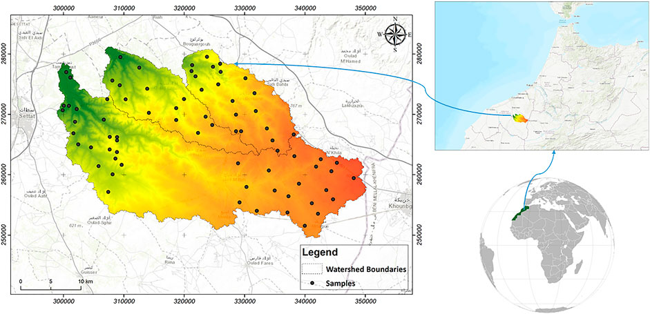
The study area is a part of the Settat-Ben Ahmed region, as three watersheds are arranged side by side, as shown in Figure 1. The most important watershed is named Tamedroust, with an area of 642.42 km²; the other two watersheds, Maze and El Himer are the smallest with 179.2 and 177.7 km², respectively. The slope is generally gentle, and the three watersheds contribute to the recharge of the Berrechid aquifer. The climate is considered semi-arid with an average annual rainfall value of 300 mm/year (Driouech, 2010), distributed generally in the rainy period, extending from October to April with maximum values of 53.1 and 48.7 mm for the months of December and January. From a pedological perspective, Calcisols dominate the surface of the three watersheds, with a limited presence of Rankers and Xerosols in El Himer watershed (Bouslihim et al., 2019).

FIGURE 1

FIGURE 1. Location of study area and distribution of sample points.

Soil Sampling and Laboratory Analysis

In this study, we adopted a stratified sampling method based on auxiliary information. Thus, 77 samples were selected based on the available soil map. Generally, we tried to ensure that all soil types were covered in the different areas, except in the middle of the Tamedroust watershed, and for that reason, we used digital mapping to produce a spatial distribution of soil aggregate stability in the entire study area. Soil samples were collected using a hand auger to collect a disturbed sample from 20 to 30 cm depth. In this regard, soil sampling standards were followed. In general. Approximately 2 kg of soil were taken from different points of the same soil and mixed in a plastic container to ensure homogeneity of the recovered sample (Proce, 1997). For SAS analysis, we adopted the standard method ISO/FDIS 10930 (2012), often known as Le Bissonnais method. Thus, only soil aggregates with diameters between 3 and 5 mm were retained and subsequently used to measured the three SAS tests (fast wetting by immersion, slow wetting by capillary action and mechanical breakdown by agitation after immersion in ethanol). These three tests present the different hydric conditions that can be encountered in the field. Fast wetting is used to compare the behavior of a wide range of soils during rapid wetting (e.g., heavy summer rainstorms). On the contrary, the slow wetting, which is less destructive than the fast wetting and can allow a better discrimination between unstable soils, corresponds to a wetting ground condition under a gentle rain. Lastly, we find the mechanical breakdown, this treatment allows to test the behavior of wet materials, generally in the wet winter periods (Le Bissonnais, 2016).

The recovered aggregates (3–5 mm) were dried in the oven for 24 h at 40°C to ensure a constant matrix potential and each test was repeated three times according to the protocol, hence for the 77 samples, we have made 693 analyses in total. The results are expressed by the mean weight diameter (MWD), which is the sum of the mass fraction of soil remaining on each sieve after sieving multiplied by the mean aperture of the adjacent mesh (Le Bissonnais, 2016).

Environmental Covariates

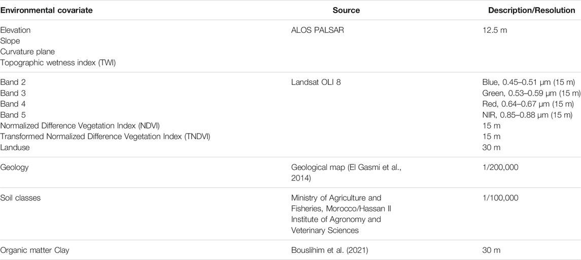
To complete the explanatory variables list, we added some environmental covariates related to soil, topography, remote sensing and additional categorical variables as geological maps, land use and soil classes (Figures 2K–M). Table 1 gives the list and characteristics of all environmental covariates used in this study.

FIGURE 2

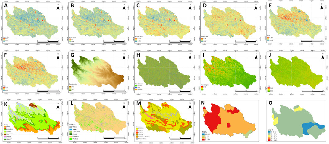
FIGURE 2. Conditioning factors used for soil aggregate stability mapping. (A) Band-2 Blue, (B) Band-3 Green, (C) Band-4 Red, (D) Band-5 NIR, (E) NDVI, (F) TNDVI, (G) Elevation, (H) Plan curvature, (I) Slope, (J) TWI, (K) Geology, (L) Landuse, (M) Soil classes, (N) Organic matter and (O) Clay.

TABLE 1

TABLE 1. Environmental covariates for soil aggregate stability prediction.

The different parameters of the topography such as elevation, slope, curvature plane and the topographic wetness index (TWI) (Figures 2G–J) were extracted with a spatial resolution of 12.5 m from the ALOS PALSAR digital elevation model acquired at https://asf.alaska.edu. The topographic covariates have been performed using the terrain analysis toolbox available in System for Automated Geoscientific Geographical Information System (SAGA-GIS) software.

For remote sensing indices, we used spectral data from the LANDSAT 8 satellite, launched in 2013 and including two sensors, namely OLI (Operational Land Imager) characterized by seven spectral bands (VNIR-SWIR) and one cirrus band with a spatial resolution of 30 m (Figures 2A–D), in addition to a panchromatic band of 15 m. The second is the Thermal Infrared Sensor (TIRS) which contains two thermal bands. Landsat-8 scenes cover 185 km × 180 km, available free of charge, with a radiometric resolution of 16 bits (Roy et al., 2014).

The Landsat 8 image (ID: LC08_L1TP_202037_20170414_20170501_01_T1), acquired on April 14, 2017, was used in the present work with L1T correction level and 0% cloud cover. The different bands are provided with the Universal Transverse Mercator (UTM) projection and the WGS 84 global geodetic system. Bands 1 and 9 are not used in this study as they are destined for atmospheric aerosol properties and cirrus detection, respectively (Roy et al., 2014; Adiri et al., 2020). The radiometric values of the spectral bands can be converted to reflectances by the following equation (Landsat Missions, 2016).

${\rho }_{{\lambda }^{\prime }}=M_{\rho }\ast Q_{cal}+A_p$

Where ρλ′ is the Top of Atmosphere Planetary Spectral Reflectance, without correction for solar angle. Mρ, Aρ and Qcal are the Reflectance multiplicative scaling factor for the band, the Reflectance additive scaling factor for the band and Level 1-pixel value in DN.

The ρλ′ is not true reflectance because it does not contain a correction for the solar elevation angle. Once a solar elevation angle is chosen, the conversion to true reflectance is as follows (Zanter, 2019):

${\rho }_{\lambda }=\frac{{\rho }_{{\lambda }^{\prime }}}{\sin \left({\theta }_{SE}\right)}$

Where ρλ is the True planetary reflectance and θ_SE is the Local sun elevation angle.

Finally, panchromatic band-8 was used to resample the OLI sensor bands at 15 m using the Pan Sharpening method “Gram-Schmidt” (Laben and Brower, 2000; Amer et al., 2012; Maurer 2013).

In semi-arid and arid regions, tracking vegetation dynamics is a significant indicator of water erosion and desertification processes. Generally, soil degradation increases when the soil has little vegetation cover. This can be quantified from remote sensing images, either by inverse modeling using radiative transfer models or using vegetation indices (Bannari, 1995). In remote sensing, the variation of the spectral response measured at the satellite sensor is an indicator of environmental change. For the quantification of vegetation cover, several vegetation indices can be used (Bouslihim et al., 2021). In the literature, the normalized difference vegetation index (NDVI) (Figure 2E) is the most popular and widely used (Mahmoudabadi et al., 2017; Maynard and Levi, 2017; Lamichhane et al., 2019). However, other indices have been developed, such as the transformed difference vegetation index (TNDVI) (Figure 2F), which quantifies vegetation cover rates more accurately than other vegetation indices (Bannari et al., 2007). NDVI and TNDVI are relatively correlated with vegetation cover rates and green biomass (Rondeaux et al., 1996).

In the present study, vegetation indices were calculated using the reflectance data of the red ρ_R and near-infrared ρ_(NIR) domains of the LANDSAT 8 satellite by the following formulas:

$NDVI=\frac{{\rho }_{NIR}-{\rho }_R}{{\rho }_{NIR}+{\rho }_R}=\frac{{\rho }_{B5}-{\rho }_{B4}}{{\rho }_{B5}+{\rho }_{B4}}$

$TNDVI= \sqrt{NDVI+0.5}$

Machine Learning Technique

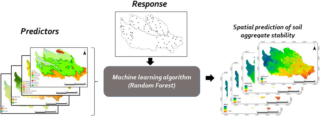
The model used in this study is an adaptation of Leo Brieman’s Random Forest (Breiman, 2001) proposed by ESRI in ArcGIS Pro program named Forest-based Classification and Regression (FCR). The power behind combining this machine learning algorithm and the ArcGIS Pro program is to take advantage of its graphical interface, which provides the user of many benefits and the ability to facilitate data preparation, explanatory data analysis, model development and model deployment. Also, this tool can be used to develop the model for both categorical variables (classification) and continuous variables (regression) based on different input data formats available. For this reason, the FCR algorithm supports different forms of explanatory variables such as tabular attributes, distance-based features, and rasters datasets. The prediction is based on creating many decision trees (forest). Each tree generates its prediction and will be used in a voting system based on the whole forest to avoid overfitting. In the current study, according to the flowchart presented in Figure 3, the model was performed using organic matter, clay, band 2, band 3, band 4, band 5, NDVI, TNDVI, elevation, slope, curvature plane and TWI as continuous variables and three categorical variables (geological maps, land use and soil classes).

FIGURE 3

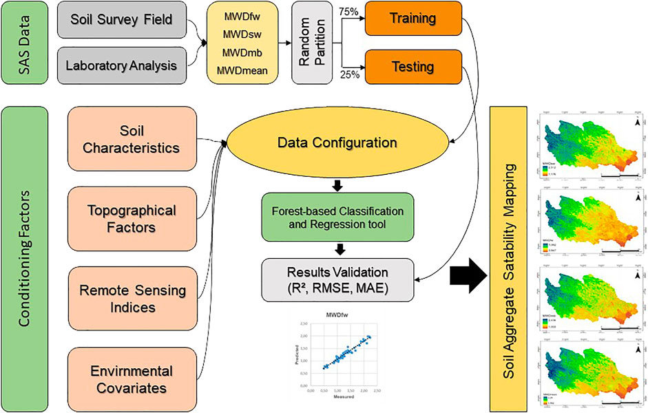
FIGURE 3. Methodological flowchart. SAS, soil aggregate stavility; MWDmb, mechanical breakdown; MWDsw, slow wetting; MWDfw, fast wetting and MWDmean, the mean of the three tests.

Model Evaluation and Accuracy Assessment

For model performance evaluation, it is necessary to randomly divide the data into two sets. For this reason, our samples (77 in total) were divided into two subsetes, where the first one acconted for 75% of the dataset (i.e., n = 57) and was used for model training. The validation was performed using the remaining 25% of the dataset (i.e., n = 20). The following equations represent the three statistical parameters that have been adopted to statistically assess the model performance. They respectively are, coefficient of determination (R²), Mean absolute error (MAE), root-mean-square error (RMSE):

$R^2=1-\frac{{\displaystyle {\sum }_{i=1}^n{\left|MWD\left(X_i\right)-MWD\left(Y_i\right)\right|}^2}}{{\displaystyle {\sum }_{i=1}^n{\left|MWD\left(X_i\right)-MWD\left(\overline{X_i}\right)\right|}^2}}$

$RMSE= \sqrt{{\displaystyle {\sum }_{i=1}^n{\left[MWD\left(X_i\right)- MWD\left(Y_i\right)\right]}^2}/n}$

$MAE=|\frac{1}{n}{\displaystyle \sum _{i=1}^n\left|MWD\left(X_i\right)-MWD\left(Y_i\right)\right|}$

where, $MWD\left(X_i\right)$ is the observed values and $MWD\left(Y_i\right)$ is the simulated values. $MWD\left(\overline{X_i}\right)$ is the mean value of observed values and n is the size of the observations.

Model with throughput resolution of prediction should display an R² value close to 1 with a low MAE and RMSE. For a classification criterion for R² values we adopted the classifications proposed by Li et al. (2016). A value of R² lower than 0.5 means an unacceptable prediction, values between 0.5 and 0.75 are acceptable and values higher than 0.75 can be considered as a good prediction.

Variable importance (input data) is also a crucial determinant of model performance, as it provides insight into each variable's contribution. However, the importance score is determined using Gini coefficients (Menze et al., 2009), which can be considered as the number of occasions a variable is responsible for a split and its impact divided by the number of trees.

Data Processing and Statistical Analysis

Prior to this analysis, original values are ln(x + 1)-transformed so they can have a comparable scale. As the multivariate statistical approaches involve all the variables in data processing thus, this two-dimensional clustered heatmap and principal component analysis (PCA) were applied using R software for comprehensive data analysis. For 2-D clustered heatmap, rows are centered; Unit variance scaling is applied to rows. Both rows and columns are clustered using correlation distance and average linkage. The color-coding within the dataset, using different colors with their intensities for positive and negative correlations, is the fundamental principle in cluster heatmapping. Weak correlations are displayed in low color intensity, while stronger ones are shown with high color intensity. Positive correlations were represented by red color, while negative ones were marked in turquoise.

Regarding the PCA method, unit variance scaling is applied to rows; Nipals PCA is used to calculate principal components. X and Y axis show principal component 1 and principal component 2, explaining 98.1 and 0.9% of the total variance, respectively. The aforementioned methods, with (PCA) and without (heatmap) dimensionality reduction, were both used to understand the network connections in a symmetric adjacency matrix and then to determine the most relevant variables in the dataset. Finally, Pearson correlation coefficients were used to determine the relationship between any two groups of variables.

Results and Discussion

Descriptive Statistics

Both clustering heatmap and PCA models that assume an unsupervised learning approach were used alongside a machine learning approach that relies on a supervised learning process to understand the network connections in the dataset and then determine the most relevant variables explaining the large variance in both models.

Data imagining is an essential mean for soil data analysis, and dimensionality reduction procedures, such as PCA, are regularly used to plot high dimensional data onto two- or three-dimensional space for better visualization. However, this approach is costly, often resulting in the loss of the total variance explained by the model. Indeed, a hierarchically clustered heatmap is among many analyses that do not require a dimensionality reduction for data visualization. It is widely used to examine complex data by displaying potential relationships in a symmetric matrix to understand the data better. The color-coded heatmap is formed with two clusters using correlation distance and average linkage; one is sample-oriented while the other is variable-oriented (Figure 4). In this figure, the output variables, including MWDmean, MWDmb, MWDfw and MWDsw, were clustered together in the same subcluster, next to which OM, clay and slope were identified as a single subcluster. These variables were found to be strongly correlated, as shown in Figure 5. However, both TNDVI and NDVI were separately classified in another subcluster alongside the variables B2, B3 and B4, to which they were negatively correlated (Figures 4, 5). The last subcluster included TWI, elevation and curvature, which displayed weak negative correlations (Figures 4, 5). Examining the clustered heatmap models shows that the variable elevation has a large effect on the model since it captured the highest amount of the total variance shared. In order of importance, the following variables clay, TWI and OM, along with slope, have largely contributed to the variance explained. Likewise, the 2-D plot of the PCA loadings showed that only the five aforementioned variables, respecting the above order of importance, have captured a large amount of total variance explained by the model (Figure 6). The sample-oriented cluster showed two main soil groups; the first one includes only seven samples, while the second was larger with 70 soil samples subdivided into three subclusters. Based on the color-coded correlation of the heatmap, the only significant difference between the two main clusters is attributed to the slope. Thus, the first cluster was characterized with a very low slope ranging between 0 and 0.51. It is noteworthy that both PCA and clustered heatmap models displayed almost similar total variance, despite being different in their respective data processing methods. This is probably due to high collinearity between the investigated variables, particularly the input variables.

FIGURE 4

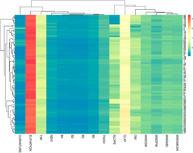
FIGURE 4. Two-dimensional clustered heatmap based on the correlation matrix of studied variables. Weak correlations are displayed in low color intensity, while stronger ones are shown with high color intensity. Positive correlations were represented by red color, while negative ones were marked in turquoise.

FIGURE 5

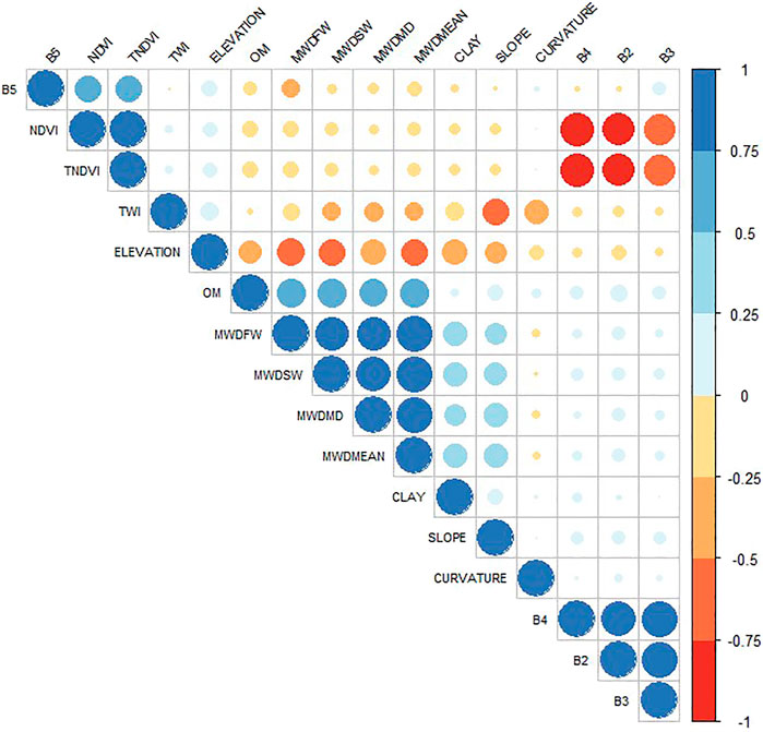
FIGURE 5. Heatmap correlations showing the relationships between investigated variables. MWDmb, mechanical breakdown; MWDsw, slow wetting; MWDfw, fast wetting; MWDmean, the mean of the three tests; OM, organic matter; NDVI, normalized difference vegetation index; TNDVI, transformed normalized difference vegetation index; B2, Band 2; B3, Band 3; B4, Band 4; B5, Band 5 and TWI, topographic wetness index.

FIGURE 6

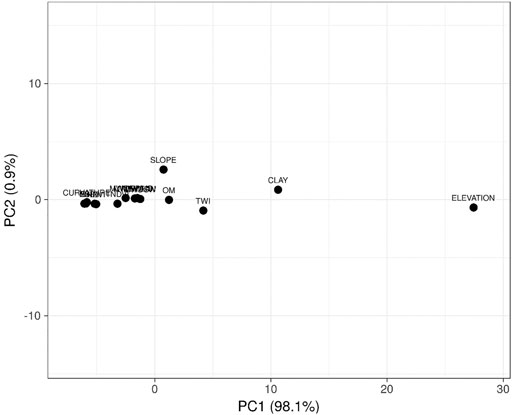
FIGURE 6. PCA scatter lot showing the variable contribution in the dataset. X and Y axis show principal component 1 and principal component 2 that explain 98.1 and 0.9% of the total variance.

Determining the Relative Importance of Variables

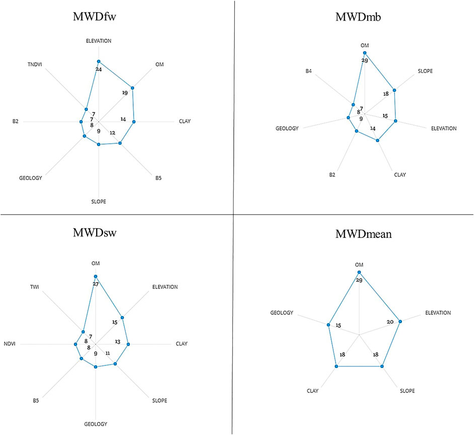
Based on Figure 7, it was observed that topography parameters and organic matter have the most contribution in predicting different MWD tests. For MWDfw, we notice that elevation was the best predicting variable with 24%, followed by OM, clay, and band 5 with 19, 14, and 12%, respectively. The other variables such as slope, geology, band 2 and TNDVI were considered as redundant attributes among the input parameters and their contribution did not overall exceed 10% (9% for slope, 8% for geology and 7% for band 2 and TNDVI). However, other parameters such as plan curvature, soil and land use have no contribution in any other model. For MWDmb and MWDsw, this time, organic matter leads the predictive variables, with values between 27 and 29%. Also, elevation, slope and clay contribute significantly to this prediction, with values ranging between 11 and 18%. For the MWDmean, Figure 7 shows a roughly balanced contribution between OM, elevation, slope, clay and geology with values ranging between 29 and 15%.

FIGURE 7

FIGURE 7. The relative importance of different variables.

Therefore, it can be determined that soil properties contribute significantly to predicting MWD, specifically organic matter. This can be supported by previous studies, which showed the high correlation between OM and SAS (Abiven et al., 2009; Chaplot and Cooper, 2015) and that OM represents a significant contributor in the prediction of MWD (Bieganowski et al., 2018; Rivera and Bonilla, 2020). Also, Annabi et al. (2017) reported the significant weight of clays in the pedotransfer-function of MWDfw, which confirms the current study’s results on the contribution of clay in the prediction of different SAS tests. This funding returns us to the important role of geology (the nature of substrates) in this prediction, which is the source of various soil properties (such as soil texture, organic matter, and proportion of different chemicals) (Annabi, et al., 2017).

Many other studies confirmed the significant role of topography and its derivatives (elevation, slope and TWI) in the spatial distribution of SAS (Cantón et al., 2009; Tang et al., 2010; Nsabimana et al., 2020). Furthermore, we cannot forget the effect of the topography on other soil properties (Kumar and Singh, 2016; Li et al., 2020; Maleki et al., 2020; Tajik el al., 2020) and distribution of vegetation (Celik, 2005; Jin et al., 2008; Mahmoudabadi et al., 2017; Maynard and Levi, 2017), which will undoubtedly affect the distribution of soil stability.

Besides all above results, we cannot forget the role of remote sensing parameters, which have shown their importance during this study. Many previous studies can also support these results (Besalatpour et al., 2014; Shi et al., 2020; Jones et al., 2021; Kamamia et al., 2021). In contrast, Bouslihim et al. (2021) reported a low contribution of remote sensing indices in estimating SAS, and this was justified by the presence of other parameters that often reduced the role of remote sensing indices. Although some studies have reported the role of climate in SAS distribution (Cerdà, 2000; Guan et al., 2018; Le Bissonnais et al., 2018), these data were not used in the current paper due to the small size of the study area and the limited spatial change for climatic conditions.

Model Accuracy

The performance results of different models were evaluated based on statistical validation indices such as R², RMSE and MAE for both training (75% of samples) and testing (25% of samples). All achieved results are listed in Table 2. According to the classification proposed by Li et al. (2016), for the training stage, the obtained R² results showed that all the models performed by FCR for the different SAS tests (MWDsw, MWDfw, MWDmb and MWDmean) are classified in the “good prediction” category (R² > 0.92). This shows that the FCR model has well modeled the different stability tests, especially for MWDsw with an R² value of 0.95. The other statistical indices (RMSE and MAE) were used to diagnose error variation. We notice that the values obtained for RMSE and MAE are low for the four implemented models, with values ranging from 0.138 to 0.158 mm for RMSE and between 0.107 and 0.119 mm for MAE. Also, the difference between the two indices is insignificant. The average differences between the predicted and the measured values of MWD was between 0.031 and 0.039 mm for the four tests. This indicates that the magnitude of the errors varies slightly, which confirms the good results obtained during the training stage.

TABLE 2

TABLE 2. FCR training and testing results for different MWD tests.

For the validation phase, we remarked a decrease in the performance of different models. According to R² classification, testing results were classified as (good prediction = R² ≥ 0.75) for MWDmean and MWDsw, with R² values of 0.8 and 0.76. In comparison, the two other models were classified as (acceptable prediction = 0.50 ≤ R² < 0.75) with R² values of 0.73 and 0.65 for MWDmb and MWDfw. The other indices (RMSE and MAE) follow the same tendency, with low values close to 0 for the four built models. Moreover, the difference between the two indices remained low and did not exceed 0.061 mm. These results show that the FCR model successfully predicted the MWD values for the different SAS tests for the validation step.

Previous studies have tried to estimate soil stability using various models and available information. However, the difference in measuring soil stability using those models remained a challenging obstacle for comparing their prediction resolutions. Indeed, the R² values reported in the current study were higher compared to thoses reported in several previous studies. Kamamia et al. (2021) obtained R² values of 0.53 and 0.39 for training and testing, respectively, using the Cubist model and 90 samples in the Ruiru watershed (Kenya). Singh et al. (2019) used Multiple Linear Regression in the Uttarakhand watershed (India) by applying a different data combination (soil, topography and soil/topography); The results obtained did not exceed 0.50 for R² for the soil and topography combination, where reported values ranged between 0.36 and 0.37 for the other models.

Contrary to aforementioned studies, Rivera and Bonilla (2020) reported good performance for the Artificial Neural Network (ANN) model with an R² value = 0.80 for training and R² = 0.82 for testing. On the other hand, Generalized Linear Model yielded acceptable results with R² values of 0.59 and 0.63 for both training and testing. Using ANN and MLR models, Marashi et al. (2017) showed the capability of the ANN model to predict MWD with an R² value of 0.87 for training and 0.93 for testing, against values of 0.78 and 0.90 for training and testing, respectively, for the MLR model. All these findings show that the results obtained during this study are encouraging, especially the stability of the model during the different phases (training and testing).

Spatial Prediction of Soil Aggregate Stability

The different environmental covariates that significantly impact model development were used in a raster format to generate spatial distribution maps using the FCR model under the ArcGIS Pro program. The best prediction map of each SAS test (MWDsw, MWDfw, MDWmb and MWDmean) are presented in Figure 8. The generated maps show the existence of unstable and medium stable soils in the southwestern part of the study area, while stable soils are found in the middle and north. The very stable soils are generally distributed in the northeast part. The effect of topography (especially elevation) on the distribution of stability indices was clearly seen. The unstable soils are found in the areas with the highest elevations (the western part), while the very stable soils are concentrated in the plain areas with the lowest elevations (the downstream part of the Mazer and Tamedroust watersheds). Besides, the effect of geology is apparent, especially for MWDmean (Figure 8D). Several MWD classes have shaped the geological layers, e.g., the Turonian in the middle of the study area, the Quaternary and Triassic in the downstream parts of the watersheds. This effect of the geological map pattern on SAS distribution was reported by Annabi et al. (2017). This was indeed expected, considering the relationship of geological factors to soil properties (Crowther, 1930; Kassai and Sisák 2018).

FIGURE 8

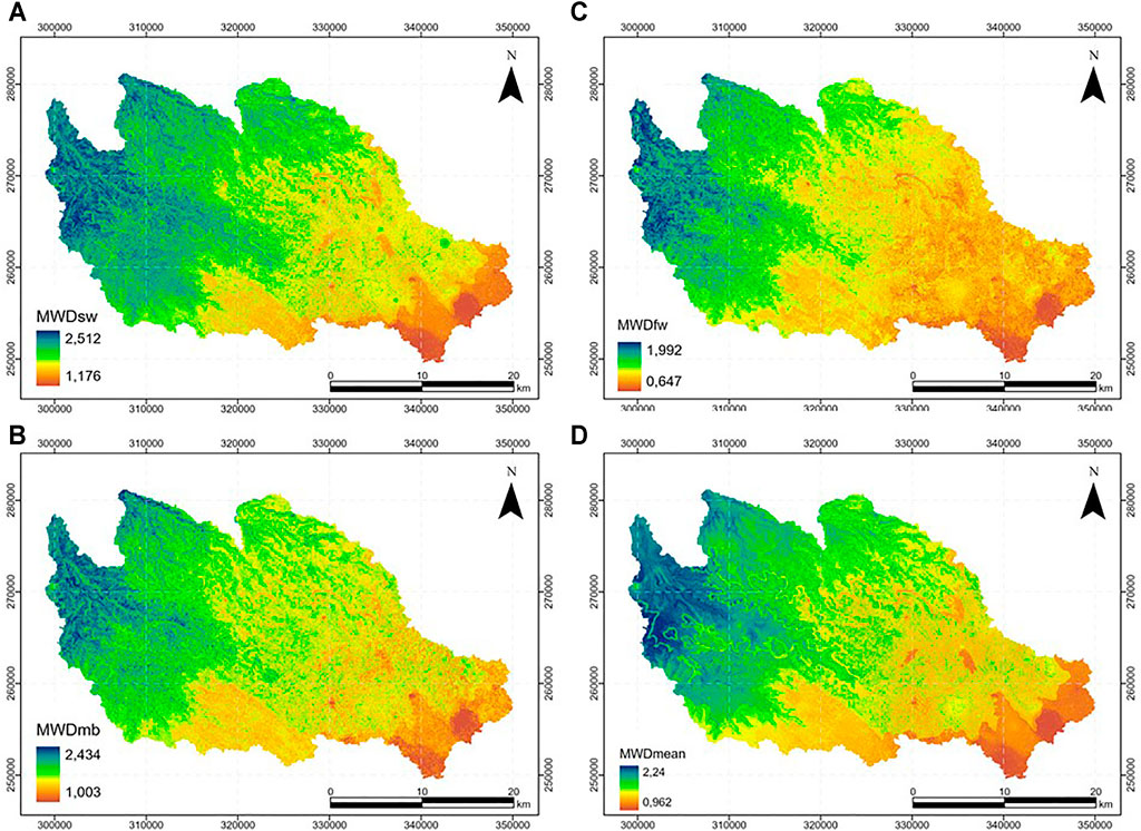
FIGURE 8. Prediction maps of soil aggregate stability: (A) MWDsw, (B) MWDmb, (C) MWDfw and (D) MWDmean.

Unlike other watersheds, the downstream part of the El Himer is characterized by the presence of stable soils for MWDmean, which is generally due to the existence of anthropogenic activities (clay quarries) and high slopes on the northeastern limb in the right tributary of El Himer river, as mentioned in the study conducted by Bouslihim et al. (2020). What is interesting is the absence of very unstable soils throughout the region (MWD < 0.4 mm) with a domination of the two classes: moderately stable (0.8 < MWD < 1.3 mm) and stable (1.3 < MWD < 2.0 mm). This can be underpinned by the findings by Bouslihim (2020), Bouslihim et al. (2021) regarding the low soil erosion rates in the region; moreover, the only exposed area to erosion is the downstream part of the El Himer watershed due to the factors mentioned earlier (anthropogenic factors and topography).

Conclusion

The model used in this study approved its capabilities to predict soil structural stability based on the MWD index with its different tests (MWDfw, MDWsw, MDWmb and MWDmean). The results obtained are satisfactory for both training and evaluation phases. The integration of the RF algorithm in the ArcGIS Pro program permitted to produce maps of the spatial distribution of the four stability tests using the model results. The generated maps showed the existence of unstable to moderately stable soils in the southwestern part, stable soils in the middle and northern part of the area, with very stable soils distributed in the northeastern part. This distribution was generally affected by a few factors such as organic matter (more than 24%), topography (specifically elevation with a percentage ranging from 15 to 24%), and geology (20% for MWDmean), with a moderate contribution from remote sensing indices and at best does not exceed 12%. In the absence of sufficient studies, further investigations under similar conditions are utmost required to verify that the same variables remain significant for mapping the stability of soil aggregates in regions characterized by a semi-arid climate. The prediction maps can be used as a basis for delineating areas of potential erosion and are very useful for management considerations. This approach can be considered an affordable methodology. However, one of the limitations of this work is that a larger sample size is required.

Data Availability Statement

The original contributions presented in the study are included in the article/Supplementary Material, further inquiries can be directed to the corresponding author.

Author Contributions

YB : methodology conceptualisation and modeling. YB, LH, AM: prepare the original draft. LH: statistical analysis. AR, RA, NAP, AM: data curation and visualisation. YB, LH: Review. All authors have read and agreed to the published version of the manuscript.

Conflict of Interest

The authors declare that the research was conducted in the absence of any commercial or financial relationships that could be construed as a potential conflict of interest.

Publisher’s Note

All claims expressed in this article are solely those of the authors and do not necessarily represent those of their affiliated organizations, or those of the publisher, the editors and the reviewers. Any product that may be evaluated in this article, or claim that may be made by its manufacturer, is not guaranteed or endorsed by the publisher.

References

Abiven, S., Menasseri, S., and Chenu, C. (2009). The Effects of Organic Inputs Over Time on Soil Aggregate Stability - A Literature Analysis. Soil Biol. Biochem. 41 (1), 1–12. doi:10.1016/j.soilbio.2008.09.015

CrossRef Full Text | Google Scholar

Adiri, Z., Lhissou, R., El Harti, A., Jellouli, A., and Chakouri, M. (2020). Recent Advances in the Use of Public Domain Satellite Imagery for mineral Exploration: A Review of Landsat-8 and Sentinel-2 Applications. Ore Geology. Rev. 117, 103332. doi:10.1016/j.oregeorev.2020.103332

CrossRef Full Text | Google Scholar

Al Masmoudi, Y., Bouslihim, Y., Doumali, K., El Aissaoui, A., and Namr, K. I. (2021). Application of the Random Forest Model to Predict the Plasticity State of Vertisols. J. Ecol. Eng. 22 (2). doi:10.12911/22998993/130878

CrossRef Full Text | Google Scholar

Amer, R., Kusky, T., and El Mezayen, A. (2012). Remote Sensing Detection of Gold Related Alteration Zones in Um Rus Area, Central Eastern Desert of Egypt. Adv. Space Res. 49 (1), 121–134. doi:10.1016/j.asr.2011.09.024

CrossRef Full Text | Google Scholar

Annabi, M., Raclot, D., Bahri, H., Bailly, J. S., Gomez, C., and Le Bissonnais, Y. (2017). Spatial Variability of Soil Aggregate Stability at the Scale of an Agricultural Region in Tunisia. Catena 153, 157–167. doi:10.1016/j.catena.2017.02.010

CrossRef Full Text | Google Scholar

Bannari, A. D. (1995). FBonn. A Rev. Vegetation Indices 13, 95r120. doi:10.1016/0264-410x(95)90122-6

CrossRef Full Text | Google Scholar

Bannari, A., Ozbakir, A., and Langlois, A. (2007). “Spatial Distribution Mapping of Vegetation Cover in Urban Environment Using TDVI for Quality of Life Monitoring,” in 2007 IEEE International Geoscience and Remote Sensing Symposium (IEEE), 679–682. doi:10.1109/igarss.2007.4422887

CrossRef Full Text | Google Scholar

Barman, U., and Choudhury, R. D. (2020). Soil Texture Classification Using Multi Class Support Vector Machine. Inf. Process. Agric. 7 (2), 318–332. doi:10.1016/j.inpa.2019.08.001

CrossRef Full Text | Google Scholar

Barthès, B., and Roose, E. (2002). Aggregate Stability as an Indicator of Soil Susceptibility to Runoff and Erosion; Validation at Several Levels. Catena 47 (2), 133–149. doi:10.1016/s0341-8162(01)00180-1

CrossRef Full Text | Google Scholar

Batjes, N. H., Ribeiro, E., van Oostrum, A., Leenaars, J., Hengl, T., and Mendes de Jesus, J. (2017). WoSIS: Providing Standardised Soil Profile Data for the World. Earth Syst. Sci. Data 9 (1), 1–14. doi:10.5194/essd-9-1-2017

CrossRef Full Text | Google Scholar

Besalatpour, A. A., Ayoubi, S., Hajabbasi, M. A., Jazi, A. Y., and Gharipour, A. (2014). Feature Selection Using Parallel Genetic Algorithm for the Prediction of Geometric Mean Diameter of Soil Aggregates by Machine Learning Methods. Arid Land Res. Manag. 28 (4), 383–394. doi:10.1080/15324982.2013.871599

CrossRef Full Text | Google Scholar

Bieganowski, A., Zaleski, T., Kajdas, B., Sochan, A., Józefowska, A., Beczek, M., et al. (2018). An Improved Method for Determination of Aggregate Stability Using Laser Diffraction. Land Degrad. Dev. 29 (5), 1376–1384. doi:10.1002/ldr.2941

CrossRef Full Text | Google Scholar

Bouslihim, Y. (2020). Hydrological and Soil Erosion Modeling Using SWAT Model and Pedotransfert Functions: A Case Study of Settat-Ben Ahmed Watersheds. Doctoral dissertation. Morocco: Université Hassan Ier Settat.

Google Scholar

Bouslihim, Y., Rochdi, A., El Amrani Paaza, N., and Liuzzo, L. (2019). Understanding the Effects of Soil Data Quality on SWAT Model Performance and Hydrological Processes in Tamedroust Watershed (Morocco). J. Afr. Earth Sci. 160, 103616. doi:10.1016/j.jafrearsci.2019.103616

CrossRef Full Text | Google Scholar

Bouslihim, Y., Rochdi, A., and El Amrani Paaza, N. (2021). Machine Learning Approaches for the Prediction of Soil Aggregate Stability. Heliyon 7 (3), e06480. doi:10.1016/j.heliyon.2021.e06480

PubMed Abstract | CrossRef Full Text | Google Scholar

Bouslihim, Y., Rochdi, A., and Paaza, N. E. A. (2020). Combining SWAT Model and Regionalization Approach to Estimate Soil Erosion under Limited Data Availability Conditions. Eurasian Soil Sc. 53 (9), 1280–1292. doi:10.1134/s1064229320090021

CrossRef Full Text | Google Scholar

Breiman, L. (2001). Random Forests. Machine Learn. 45 (1), 5–32. doi:10.1023/a:1010933404324

CrossRef Full Text | Google Scholar

Bünemann, E. K., Bongiorno, G., Bai, Z., Creamer, R. E., De Deyn, G., de Goede, R., et al. (2018). Soil Quality - A Critical Review. Soil Biol. Biochem. 120, 105–125. doi:10.1016/j.soilbio.2018.01.030

CrossRef Full Text | Google Scholar

Cantón, Y., Solé-Benet, A., Asensio, C., Chamizo, S., and Puigdefábregas, J. (2009). Aggregate Stability in Range sandy Loam Soils Relationships with Runoff and Erosion. Catena 77 (3), 192–199. doi:10.1016/j.catena.2008.12.011

CrossRef Full Text | Google Scholar

Celik, I. (2005). Land-Use Effects on Organic Matter and Physical Properties of Soil in a Southern Mediterranean highland of Turkey. Soil Tillage Res. 83 (2), 270–277. doi:10.1016/j.still.2004.08.001

CrossRef Full Text | Google Scholar

Cerdà, A. (2000). Aggregate Stability Against Water Forces under Different Climates on Agriculture Land and Scrubland in Southern Bolivia. Soil Tillage Res. 57 (3), 159–166. doi:10.1016/s0167-1987(00)00155-0

CrossRef Full Text | Google Scholar

Chaplot, V., and Cooper, M. (2015). Soil Aggregate Stability to Predict Organic Carbon Outputs from Soils. Geoderma 243–244, 205–213. doi:10.1016/j.geoderma.2014.12.013

PubMed Abstract | CrossRef Full Text | Google Scholar

Crowther, E. M. (1930). The Relationship of Climatic and Gelogical Factors to the Composition of Soil clay and the Distribution of Soil Types. Proc. R. Soc. Lond. B. 107 (748), 1–30. doi:10.1098/rspb.1930.0049

CrossRef Full Text | Google Scholar

De La Rosa, D. (2003). Soil Quality Evaluation and Monitoring. Soil Conservation and Protection for Europe, 64. Alicante, Spain: The first SCAPE workshop.

Delelegn, Y. T., Purahong, W., Blazevic, A., Yitaferu, B., Wubet, T., Göransson, H., et al. (2017). Changes in Land Use Alter Soil Quality and Aggregate Stability in the highlands of Northern Ethiopia. Sci. Rep. 7 (1), 13602–13612. doi:10.1038/s41598-017-14128-y

PubMed Abstract | CrossRef Full Text | Google Scholar

Dokuchaev, V. V. (1967). Russian Chernozem-Selected Works of VV Dokuchaev. Jerusalem: Translated from the Russian by Israel Program for Scientific Translations.

Driouech, F. (2010). Distribution des précipitations hivernales sur le Maroc dans le cadre d’un changement climatique: descente d'échelle et incertitudes. Doctoral dissertation. Institut National Polytechnique de Toulouse.

Google Scholar

El Gasmi, H., Mridekh, A., Tammal, M., and El bouhaddiouI, M. (2014). Apport des données géophysiques et géologiques à la mise en évidence de nouveaux éléments structuraux associés à la flexure de Settat (Maroc central) Contribution of geophysical and geological data for the identification of new structural elements related to the Settat flexure (central Morocco). Bull. l’Inst. Sci. Rabat 36.

Google Scholar

Fick, S. E., and Hijmans, R. J. (2017). WorldClim 2: New 1‐km Spatial Resolution Climate Surfaces for Global Land Areas. Int. J. Climatol. 37 (12), 4302–4315. doi:10.1002/joc.5086

CrossRef Full Text | Google Scholar

González-Moradas, M. d. R., and Viveen, W. (2020). Evaluation of ASTER GDEM2, SRTMv3.0, ALOS AW3D30 and TanDEM-X DEMs for the Peruvian Andes against Highly Accurate GNSS Ground Control Points and Geomorphological-Hydrological Metrics. Remote Sens. Environ. 237, 111509. doi:10.1016/j.rse.2019.111509

CrossRef Full Text | Google Scholar

Guan, S., An, N., Zong, N., He, Y., Shi, P., Zhang, J., et al. (2018). Climate Warming Impacts on Soil Organic Carbon Fractions and Aggregate Stability in a Tibetan alpine Meadow. Soil Biol. Biochem. 116, 224–236. doi:10.1016/j.soilbio.2017.10.011

CrossRef Full Text | Google Scholar

Hengl, T., and MacMillan, R. A. (2019). Predictive Soil Mapping with R. Wageningen, Netherlands: OpenGeoHub Foundation.

Hengl, T., Mendes de Jesus, J., Heuvelink, G. B. M., Ruiperez Gonzalez, M., Kilibarda, M., Blagotić, A., et al. (2017). SoilGrids250m: Global Gridded Soil Information Based on Machine Learning. PLoS one 12 (2), e0169748. doi:10.1371/journal.pone.0169748

PubMed Abstract | CrossRef Full Text | Google Scholar

Jenny, H. (1941). Factors of Soil Formation. A System of Quantitative Pedology. New York: McGraw-Hill Book Co.

Jin, X. M., Zhang, Y. K., Schaepman, M. E., Clevers, J. G. P. W., Su, Z., Cheng, J., et al. (2008). “Impact of Elevation and Aspect on the Spatial Distribution of Vegetation in the Qilian Mountain Area with Remote Sensing Data,” in International Society for Photogrammetry and Remote Sensing (Beijing: ISPRS), 1385–1390.

Google Scholar

Jones, E. J., Filippi, P., Wittig, R., Fajardo, M., Pino, V., and McBratney, A. B. (2021). Mapping Soil Slaking index and Assessing the Impact of Management in a Mixed Agricultural Landscape. Soil 7 (1), 33–46. doi:10.5194/soil-7-33-2021

CrossRef Full Text | Google Scholar

Kamamia, A. W., Vogel, C., Mwangi, H. M., Feger, K.-H., Sang, J., and Julich, S. (2021). Mapping Soil Aggregate Stability Using Digital Soil Mapping: A Case Study of Ruiru Reservoir Catchment, Kenya. Geoderma Reg. 24, e00355. doi:10.1016/j.geodrs.2020.e00355

CrossRef Full Text | Google Scholar

Karlen, D. L., Ditzler, C. A., and Andrews, S. S. (2003). Soil Quality: Why and How?. Geoderma 114 (3–4), 145–156. doi:10.1016/s0016-7061(03)00039-9

CrossRef Full Text | Google Scholar

Kassai, P., and Sisák, I. (2018). The Role of Geology in the Spatial Prediction of Soil Properties in the Watershed of Lake Balaton, Hungary. Geol. Cro 71 (1), 29–39. doi:10.4154/gc.2018.04

CrossRef Full Text | Google Scholar

Kumar, S., and Singh, R. P. (2016). Spatial Distribution of Soil Nutrients in a Watershed of Himalayan Landscape Using Terrain Attributes and Geostatistical Methods. Environ. Earth Sci. 75 (6), 473. doi:10.1007/s12665-015-5098-8

CrossRef Full Text | Google Scholar

Laben, C. A., and Brower, B. V. (2000). U.S. Patent No. 6011875. Washington, DC: U.S. Patent and Trademark Office.

Lagacherie, P. (2008). Digital Soil Mapping: A State of the Art. Digital Soil Mapping with Limited Data. Springer, 3–14.

Lamichhane, S., Kumar, L., and Wilson, B. (2019). Digital Soil Mapping Algorithms and Covariates for Soil Organic Carbon Mapping and Their Implications: A Review. Geoderma 352, 395–413. doi:10.1016/j.geoderma.2019.05.031

CrossRef Full Text | Google Scholar

Landsat Missions (2016). Landsat Missions: Using the USGS Landsat 8 Product. Available at: https://landsat.usgs.gov/using-usgs-landsat-8-product.

Google Scholar

László, M. (2009). “Main Parameters of Soil Quality and it’s Management under Changing Climate,” in EGU General Assembly Conference Abstracts, Vienna, Austria, 1400.

Google Scholar

Le Bissonnais, Y. (2016). Aggregate Stability and Assessment of Soil Crustability and Erodibility: I. Theory and Methodology. Eur. J. Soil Sci. 67 (1), 11–21. doi:10.1111/ejss.4_12311

CrossRef Full Text | Google Scholar

Le Bissonnais, Y., Prieto, I., Roumet, C., Nespoulous, J., Metayer, J., Huon, S., et al. (2018). Soil Aggregate Stability in Mediterranean and Tropical Agro-Ecosystems: Effect of Plant Roots and Soil Characteristics. Plant and Soil 424 (1), 303–317. doi:10.1007/s11104-017-3423-6

CrossRef Full Text | Google Scholar

Li, L., Lu, J., Wang, S., Ma, Y., Wei, Q., Li, X., et al. (2016). Methods for Estimating Leaf Nitrogen Concentration of winter Oilseed Rape (Brassica napus L.) Using In Situ Leaf Spectroscopy. Ind. Crops Prod. 91, 194–204. doi:10.1016/j.indcrop.2016.07.008

CrossRef Full Text | Google Scholar

Li, X., McCarty, G. W., Du, L., and Lee, S. (2020). Use of Topographic Models for Mapping Soil Properties and Processes. Soil Syst. 4 (2), 32. doi:10.3390/soilsystems4020032

CrossRef Full Text | Google Scholar

Ma, Y., Minasny, B., Malone, B. P., and Mcbratney, A. B. (2019). Pedology and Digital Soil Mapping (DSM). Eur. J. Soil Sci. 70 (2), 216–235. doi:10.1111/ejss.12790

CrossRef Full Text | Google Scholar

Magdoff, F. (2018). “Soil Quality and Management,” in Agroecology. (Boca Raton, FL: CRC Press), 349–364. doi:10.1201/9780429495465-18

CrossRef Full Text | Google Scholar

Mahmoudabadi, E., Karimi, A., Haghnia, G. H., and Sepehr, A. (2017). Digital Soil Mapping Using Remote Sensing Indices, Terrain Attributes, and Vegetation Features in the Rangelands of Northeastern Iran. Environ. Monit. Assess. 189 (10), 500–520. doi:10.1007/s10661-017-6197-7

PubMed Abstract | CrossRef Full Text | Google Scholar

Maleki, S., Khormali, F., Mohammadi, J., Bogaert, P., and Bagheri Bodaghabadi, M. (2020). Effect of the Accuracy of Topographic Data on Improving Digital Soil Mapping Predictions with Limited Soil Data: an Application to the Iranian Loess Plateau. Catena 195, 104810. doi:10.1016/j.catena.2020.104810

CrossRef Full Text | Google Scholar

Marashi, M., Torkashvand, A. M., Ahmadi, A., and Esfandyari, M. (2017). Estimation of Soil Aggregate Stability Indices Using Artificial Neural Network and Multiple Linear Regression Models. Spanish J. Soil Sci. SJSS 7 (2), 122–132. doi:10.3232/SJSS.2017.V7.N2.04

CrossRef Full Text | Google Scholar

Maurer, T. (2013). How to Pan-Sharpen Images Using the Gram-Schmidt Pan-Sharpen Method–A Recipe. Int. Arch. photogrammetry, remote sensing Spat. Inf. Sci. 1, W1. doi:10.5194/isprsarchives-XL-1-W1-239-2013

CrossRef Full Text | Google Scholar

Maynard, J. J., and Levi, M. R. (2017). Hyper-Temporal Remote Sensing for Digital Soil Mapping: Characterizing Soil-Vegetation Response to Climatic Variability. Geoderma 285, 94–109. doi:10.1016/j.geoderma.2016.09.024

CrossRef Full Text | Google Scholar

McBratney, A. B., Santos, M. M., and Minasny, B. (2003). On Digital Soil Mapping. Geoderma 117 (1-2), 3–52. doi:10.1016/s0016-7061(03)00223-4

CrossRef Full Text | Google Scholar

McKenzie, B. M., Tisdall, J. M., and Vance, W. H. (2011). “Soil Physical Quality,” in Encyclopedia of Agrophysics. Encyclopedia of Earth Sciences Series. Editors J. Gliński, J. Horabik, and J. Lipiec (Dordrecht: Springer), 770–777. doi:10.1007/978-90-481-3585-1_153

CrossRef Full Text | Google Scholar

Melnik, M. S., Podkolzin, O. A., Yu Perov, A., and Odintsov, S. V. (2019). Monitoring and Certification of Agricultural Land by Creating a Bank of Information Resources for the Rational Use of Steppe Landscapes of the Western Ciscaucasia. IOP Conf. Ser. Earth Environ. Sci. 315, 032028. doi:10.1088/1755-1315/315/3/032028

CrossRef Full Text | Google Scholar

Menze, B. H., Kelm, B. M., Masuch, R., Himmelreich, U., Bachert, P., Petrich, W., et al. (2009). A Comparison of Random forest and its Gini Importance with Standard Chemometric Methods for the Feature Selection and Classification of Spectral Data. BMC Bioinformatics 10 (1), 213–216. doi:10.1186/1471-2105-10-213

PubMed Abstract | CrossRef Full Text | Google Scholar

Nabiollahi, K., Golmohamadi, F., Taghizadeh-Mehrjardi, R., Kerry, R., and Davari, M. (2018). Assessing the Effects of Slope Gradient and Land Use Change on Soil Quality Degradation through Digital Mapping of Soil Quality Indices and Soil Loss Rate. Geoderma 318, 16–28. doi:10.1016/j.geoderma.2017.12.024

CrossRef Full Text | Google Scholar

Nsabimana, G., Bao, Y., He, X., Nambajimana, J. d. D., Wang, M., Yang, L., et al. (2020). Impacts of Water Level Fluctuations on Soil Aggregate Stability in the Three Gorges Reservoir, China. Sustainability 12 (21), 9107. doi:10.3390/su12219107

CrossRef Full Text | Google Scholar

Proce, G. (1997). Soil Sampling. Lancaster, New York: Ecology and Environment, Inc.

Qiao, X., Wang, C., Feng, M., Zhang, M., Song, X., Xiao, L., et al. (2021). Hyperspectral Response and Quantitative Estimation on Soil Aggregate Characters. Catena 202, 105286. doi:10.1016/j.catena.2021.105286

CrossRef Full Text | Google Scholar

Rivera, J. I., and Bonilla, C. A. (2020). Predicting Soil Aggregate Stability Using Readily Available Soil Properties and Machine Learning Techniques. Catena 187, 104408. doi:10.1016/j.catena.2019.104408

CrossRef Full Text | Google Scholar

Rondeaux, G., Steven, M., and Baret, F. (1996). Optimization of Soil-Adjusted Vegetation Indices. Remote Sensing Environ. 55, 95–107. doi:10.1016/0034-4257(95)00186-7

CrossRef Full Text | Google Scholar

Roy, D. P., Wulder, M. A., Loveland, T. R., C.E., W., Allen, R. G., Anderson, M. C., et al. (2014). Landsat-8: Science and Product Vision for Terrestrial Global Change Research. Remote Sens. Environ. 145, 154–172. doi:10.1016/j.rse.2014.02.001

CrossRef Full Text | Google Scholar

Santra, P., Kumar, M., and Panwar, N. (2017). Digital Soil Mapping of Sand Content in Arid Western India through Geostatistical Approaches. Geoderma Reg. 9, 56–72. doi:10.1016/j.geodrs.2017.03.003

CrossRef Full Text | Google Scholar

Sepuru, T. K., and Dube, T. (2018). Understanding the spatial distribution of eroded areas in the former rural homelands of South Africa: Comparative evidence from two new non-commercial multispectral sensors. Int. J. Appl. Earth Obser. Geoinfor. 69, 119–132.

CrossRef Full Text | Google Scholar

Seybold, C. A., and Herrick, J. E. (2001). Aggregate Stability Kit for Soil Quality Assessments. Catena 44 (1), 37–45. doi:10.1016/s0341-8162(00)00175-2

CrossRef Full Text | Google Scholar

Shi, P., Castaldi, F., van Wesemael, B., and Van Oost, K. (2020). Large-scale, High-Resolution Mapping of Soil Aggregate Stability in Croplands Using APEX Hyperspectral Imagery. Remote Sens. 12 (4), 666. doi:10.3390/rs12040666

CrossRef Full Text | Google Scholar

Silva, B. P. C., Silva, M. L. N., Avalos, F. A. P., de Menezes, M. D., and Curi, N. (2019). Digital Soil Mapping Including Additional point Sampling in Posses Ecosystem Services Pilot Watershed, South Eastern Brazil. Sci. Rep. 9 (1), 13763–13812. doi:10.1038/s41598-019-50376-w

PubMed Abstract | CrossRef Full Text | Google Scholar

Singh, A. K., Kumar, S., and Kalambukattu, J. G. (2019). Assessing Aggregate Stability of Soils under Various Land Use/land Cover in a Watershed of Mid-himalayan Landscape. Eurasian J. Soil Sci. 8 (2), 131–143. doi:10.18393/ejss.541319

CrossRef Full Text | Google Scholar

Tajik, S., Ayoubi, S., and Zeraatpisheh, M. (2020). Digital Mapping of Soil Organic Carbon Using Ensemble Learning Model in Mollisols of Hyrcanian Forests, Northern Iran. Geoderma Reg. 20, e00256. doi:10.1016/j.geodrs.2020.e00256

CrossRef Full Text | Google Scholar

Tang, X., Liu, S., Liu, J., and Zhou, G. (2010). Effects of Vegetation Restoration and Slope Positions on Soil Aggregation and Soil Carbon Accumulation on Heavily Eroded Tropical Land of Southern China. J. Soil. Sediment. 10 (3), 505–513. doi:10.1007/s11368-009-0122-9

CrossRef Full Text | Google Scholar

Wadoux, A. M. J.-C., Minasny, B., and McBratney, A. B. (2020). Machine Learning for Digital Soil Mapping: Applications, Challenges and Suggested Solutions. Earth Sci. Rev. 210, 103359. doi:10.1016/j.earscirev.2020.103359

CrossRef Full Text | Google Scholar

Zanter, K. (2019). Landsat 8 (L8) Data Users Handbook LSDS-1574 Version 5.0. Sioux Falls, SD: Department of the Interior.

Zeraatpisheh, M., Jafari, A., Bagheri Bodaghabadi, M., Ayoubi, S., Taghizadeh-Mehrjardi, R., Toomanian, N., et al. (2020). Conventional and Digital Soil Mapping in Iran: Past, Present, and Future. Catena 188, 104424. doi:10.1016/j.catena.2019.104424

CrossRef Full Text | Google Scholar