Occurrences of Deep-Seated Creeping Landslides in Accordance with Hydrological Water Storage in Catchments

Rainfall is one of the most important triggers of both shallow debris flows and deep-seated landslides. The triggering mechanism involves the process of water infiltration into the failure zone. For deep-seated landslides, the deeper and more extensive failure surfaces delay the effect of the process and thus delay landslide initiations. The delay is difficult to assess, especially if the sites only have scarce or insufficient monitoring data. Under these circumstances, we illustrate that the occurrences of landslides can be estimated by their correlations with the phenomenological water storage index (WSI) of a given catchment. In the present study, a total of five deep-seated landslides in TienChih (4) and SiangYang (1) are investigated. The displacements of the landslides were recorded by global positioning system (GPS) and the WSI was modelled using the tank model. The result demonstrates that the WSI correlates closer in time to the landslide motion than the rainfall, and the WSI thresholds for the landslides are inferred. Thus, this technique can be applied as an associated method to evaluate landslide initiation.

1 Introduction

Recently, in Taiwan, with continuous global positioning system (GPS) network data, eight deep-seated creeping landslide sites were identified and their causes were associated with hydrological loading, Hsu et al. (2014). The evidence was based on relating the creeping landslide events to the rainfall intensity (RI) or accumulated precipitation. In this paper, we further inspect the landslide events with a simple phenomenological quantitative hydrological model. The model, known as the tank model of Sugawara and Funiyuki (1956) and Sugawara (1961, 1995), can provide a simple idealized sketch for a regional water cycle: including precipitation, infiltration and runoff discharge. Using the model, we attempt to identify model thresholds for landslide occurrences and observe the sequential relationship between the landslides and regional water cycle.

Because of the wide extent area and deep failure surface of deep-seated landslides, the rainfall triggering mechanism involve delicate infiltration processes with site geological conditions. Detail investigations of the infiltrated water flows, however, can involve sophisticated techniques. For example, Cappa et al. (2004) traced sulfate, nitrate concentration and spring waters on the slope to identify the characteristics of precipitation infiltration and concluded that landslide motions correlate to precipitation. Padilla et al. (2014) measured electrical conductivity, oxygen and hydrogen isotopic concentration of the groundwater and correlated the recharged groundwater to rainfall. The infiltration is found to be associated with high hydraulic conductivity area in the bedrock caused by the gravitational deformation in the investigated hillslope. Lv et al. (2019) applied tracer test, injection test and electrical resistivity tomography to resolve the underground water flow in their study area. The landslide is found mainly controlled by a vertical preferential flow pathway, one of the two major types of underground water flow patterns of the site. Zêzere et al. (2005) analyzed a series of long-term monitoring data since 1950s on the occurrences of rainfall induced shallow and deep landslides. The deep-seated landslides correlate to long period but less intensive rainfalls and it indicates that the infiltration causes the rise of groundwater table and the deep failures through reduction of shear strength of the slope materials. Nie et al. (2017) extended a tank model to include effects of snow accumulation, snowmelt and infiltration. These effects resulted in time lags and the model improved the groundwater level predictions in deep-seated landslides.

To adapt a simple tank model in the present study is because the landslides were in remote areas where detailed geological surveys and field observation data required to constrain sophisticated models are scarce or insufficient. In addition, because the lack of field data is common in the mountainous areas of Taiwan Island, a simple model can be a valuable tool that can be incorporated into hazard mitigation systems if its applicability is validated. For this purpose, we selected two landslide sites: the TienChih and SiangYang areas. Provided that a minimum set of hydrological data is available, the selection criteria are described as follows: the sites are in the catchments of streams of the lowest-possible order (furthest upstream); the catchments are as small as possible; and the landslide is of the translational type, according to the landslide classification in Varnes (1978). The concept of applications of the tank model was first tested feasible in a preliminary study of the TienChih area, Lin et al. (2017), and is extended in the present paper.

Both sites are on the southern transverse roadway. The roadway was built in the 1970s to connect the southwest (Kaohsiung City) and southeast (Taitung County) parts of the island. The total length of the roadway is approximately 209 km and most of the mountainous section of the roadway is in Yushan National Park. The highest elevation of the roadway is 2,722 m at approximately 147.5 km along the roadway. On the immediate west side (Kaohsiung side) of the peak point, Yakou, the terrain is in the catchment of the Laonung River and, on the east (Taitung side), the terrain is the Beinan River catchment. The Laonung River flows to the southwest, and the Beinan River flows to the southeast. The upstream-most flow-rate-monitored catchments of the studied regions are plotted in Figure 1A. The river flow rate observation stations for the two catchments are A-Chi-Ba Bridge and Hsin-Wu-Lu. Their monitoring catchment areas are 411 and 628 km², respectively. In the catchments, there are two and four rainfall monitoring stations, as marked in the figure. However, for simplicity, only the data recorded by the rainfall station closest to the landslide site are used to represent precipitation in each catchment in the current analysis. The adapted rainfall stations are marked in Figure 2.

FIGURE 1

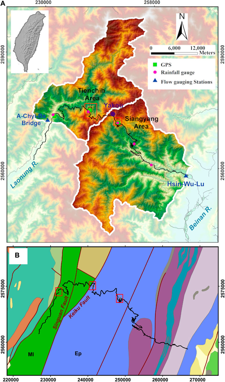
FIGURE 1. (A) The upstream catchments and the section of the south transverse highway in the study area (thick solid black line). The highlighted northwest area is the 411 km² TienChih catchment and the southeast area is the 628 km² SiangYang catchment. The landslide sites, the TienChih and SiangYang areas, are marked by thick hollow red boxes. The coordinate system is TWD97. (B) The regional fault system and lithology. MI, Miocene argillite, slate, phyllite; Ep, Eocene slate, phyllite.

FIGURE 2

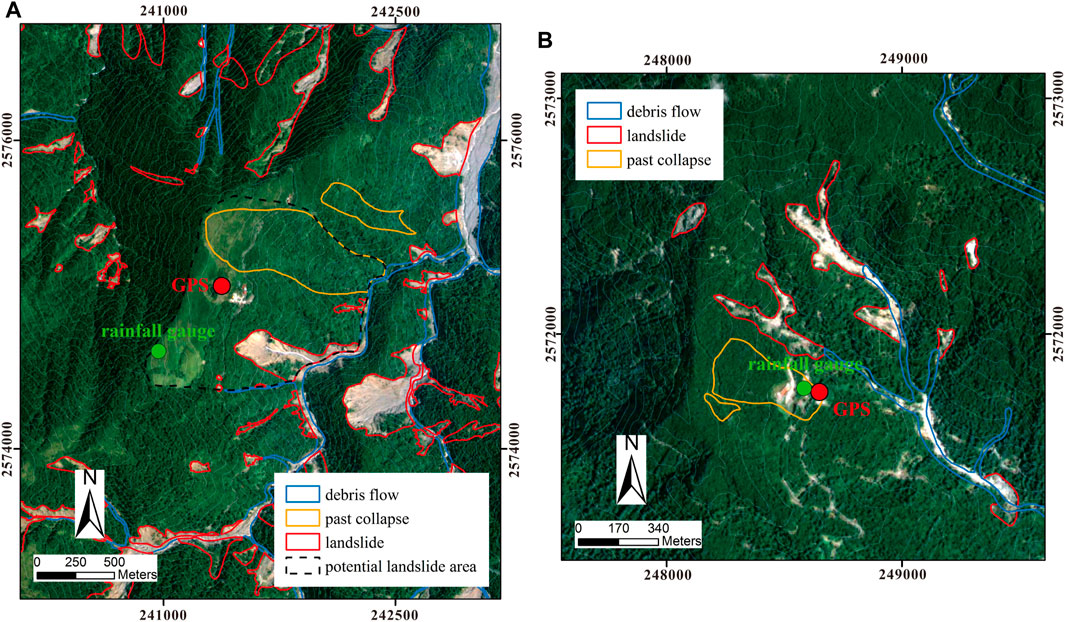
FIGURE 2. Birds-eye views of the (A) TienChih and (B) SiangYang landslide areas. The aerophotos are taken in the year 2010. The rainfall and GPS stations used in the present analysis are marked, and the landslide scars and debris flow courses are outlined. The codenames of the GPS stations are TENC and SYAN for the TienChih and SiangYang areas, respectively.

The geological settings are shown in Figure 1B. The roadway cuts through two primary faults, the Singuan and Keiku Faults, in the south Central Mountain Range, adjoined with abundant secondary named or unnamed faults, according to Lee and Wang (1985); Lai et al. (1989) and Lin (2012). These faults are mainly of the thrust type and are arranged in the NNW-SSE direction. The geological layer at both sites is the Pilu Formation. The formation extends from NNE to SSW along the ridges of the Central Mountains, as marked in the light blue colour in Figure 1B. The formation mainly consists of Eocene rocks: slate and phyllite. Moving westward from the TienChih site, the surface layer changes to the Miocene Lushan Formation (argillite, slate, phyllite), and towards the east from the SiangYang site, it becomes Late Paleozoic and Mesozoic Tananao schists (black/green/siliceous schist). These rocks all have rich joint, cleavage and fold structures which indicates an active orogenous mechanism in the region. The common filling material in the Pilu Formation is quartz-rich calcite Lai et al. (1989), which generally has high water permeability.

The locations of the TienChih and SiangYang creeping landslide sites are marked in Figure 1 and they are enlarged in Figure 2. Both sites were designed as resting and sightseeing areas on the roadway such that facilities, including a few monitoring instruments, were constructed. Therefore, creeping landslides were found by the installed instruments. The displacement measurements and field observations will be reported in the next section.

2 GPS Network and Identification of Creeping Landslides

GPSs have been gaining widespread use in real-time monitoring of surface displacements. With proper postprocessing procedures, continuous GPS (CGPS) data can achieve an accuracy of several millimetre. The data presented in this section were acquired from the island-wide GPS network constructed by the Institute of Earth Sciences, Academia Sinica and Central Weather Bureau since 1989, Yu et al. (1997, 2003); Chen et al. (2015). At the TienChih site, a CGPS station that is codenamed TENC, was set up, and recording started in 2002. At the SiangYang site, a similar station known as SIANY, started operating in 2009.

The postprocessing procedures of the collected GPS data were performed in the framework of GAMIT/GLOBK software, version 10.3, Herring et al. (2002). Double-difference phase observables were used and the influences of tropospheric and ionospheric effects were corrected. To obtain an accurate and consistent regional deformation pattern in Taiwan, a total data of 362 Taiwan and 17 IGS Asia-Pacific CGPS sites were used. The least squares linear fit was used to identify the tectonic linear station velocity, annual and semiannual periodic motions, postseismic relaxation, and offsets caused by coseismic jumps and instrument changes in the station position time series, Altamimi et al. (2007). Then, the statistical outliers, linear velocities, postseismic relaxation, and instrumental offsets were removed.

The residual GPS position time series of both stations are plotted in Figure 3. They exhibited several clearly identifiable intermittent displacements, of which TENC recorded four because of its longer period in operation. These intermittent displacements were correlated with extreme precipitation events: 6/29/2004 (Month/Day/Year) Mindulle typhoon, 7/18/2005 Haitang typhoon, 5/17/2006 heavy rainfall and 8/7/2009 Morakot typhoon. The successive displacements indicated that TENC moved unidirectionally towards the southeast-east (SEE) between 2002 and 2012. The extreme typhoon Morakot caused displacements with east, north and vertical components of 245, −49, −243 mm, respectively. SIANY also moved towards SEE after the Morakot typhoon. The displacement directions of the two sites are shown in Figure 4 which correspond exactly to the descending direction of the slopes, i.e., translational landslide. Because of poor climate conditions (typhoons, heavy clouds and rainfall) when landslides are in motion, GPS stations may not obtain data, site accessibility is lost or instrumental damage occurs. The breaks in data impede hydrological analysis, except for the unique recordings taken in the Morakot event, cf. Figure 10.

FIGURE 3

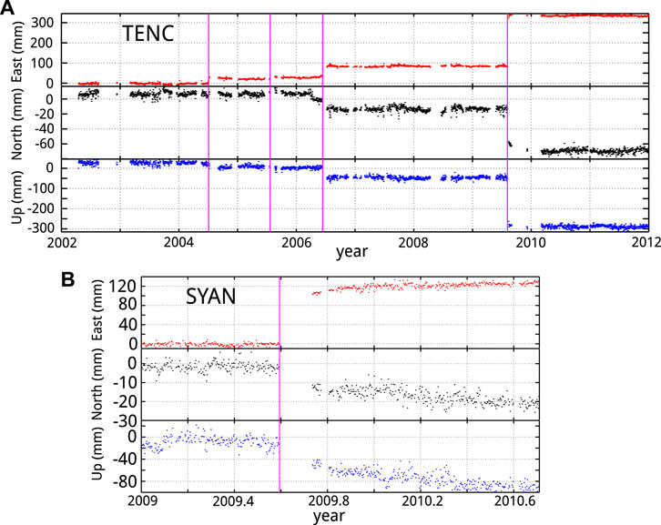
FIGURE 3. Residual GPS position time series of (A) TienChih and (B) SiangYang landslide areas. The vertical magenta lines mark the landslide events: 6/29/2004 (Month/Day/Year) Mindulle typhoon, 7/18/2005 Haitang typhoon, 5/17/2006 heavy rainfall and 8/7/2009 Morakot typhoon. Note that the horizontal time axes are on different scales.

FIGURE 4

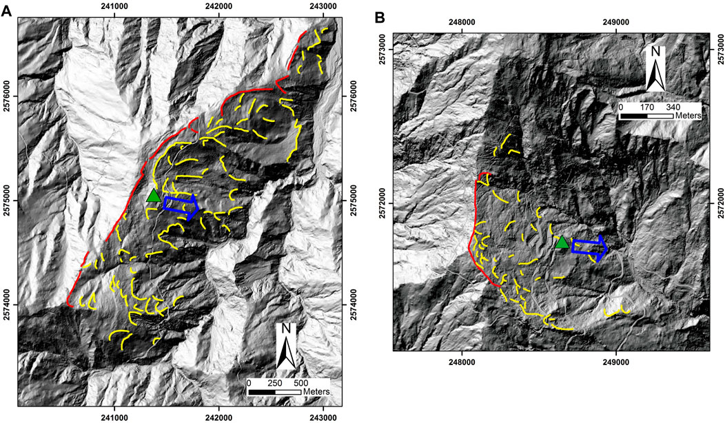
FIGURE 4. LiDAR image of topographic characteristics of the (A) TienChih and (B) SiangYang sites. Red thick line: main cracks, yellow lines: minor cracks. The GPS recorded sliding direction, 8/7/2009 ∼ 8/12/2009, is marked by the blue arrow.

The cumulative rainfall of Morakot typhoon was reached 2,700 mm in 5 days. The amount of precipitation was almost equal to the average annual rainfall on the island. This typhoon resulted in numerous landslides, excessive floods and severe fatalities in the southern part of Taiwan and after the strike, a series of light detection and ranging (LiDAR) surveys was performed over that area in 2010 by the Central Geological Survey. The LiDAR technique produces high-resolution digital elevation models (DEMs) and is superior in terms of high-precision and vegetation-penetrating capacities. The derived DEM of the LiDAR survey had a grid size with a 1 × 1 m resolution based on the average point cloud density of 0.5 point/m². For the two landslide sites, the DEMs are shown in Figure 4.

With high-resolution DEMs, surface cleavages, scarps and outcrops can be visually identified in the indoor preparation phase prior to field geological surveys. As shown in Figure 4, typical sackungen structures are found along ridge crests in massive competent rocks, running parallel to the slope contours and to the strikes of main rock discontinuities (foliation). Surface failure usually develops steep into the mountainside by gravitational stresses; therefore, scarps are created. For example, Figure 5A presents the slope profile of a shallow landslide area after the Morakot typhoon (the central scarp near the rainfall gauge marked in Figure 2A). A typical cleavage structure (fault gouge zone) in the area and underground water seepage are shown. Figure 5B illustrates the crack openings found in the main building site of the roadway rest area. The movements, although slow (long-term gravity-driven creep), can continue for long periods in principle, producing significant cumulative displacements.

FIGURE 5

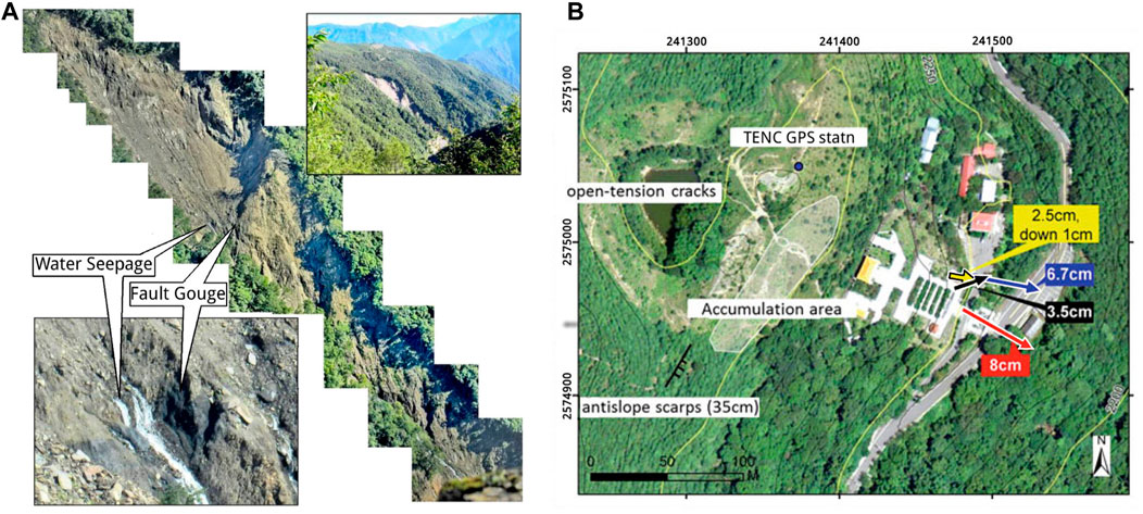
FIGURE 5. (A) The slope profile of a shallow landslide in the TienChih area after the Morakot typhoon, (the central scarp near the rainfall gauge marked in Panel 2A). A typical cleavage structure (fault gouge zone) in the area and underground water seepage are shown. (B) Crack openings in the main building site of the roadway rest area.

In the preliminary study? Chen et al. (2015), we visually examine the correlation between the temporal variation in GPS displacement time series and rainfall data (intensity and accumulated). The displacement takes place with a time lag compared with the rainfall hydrographs. This phenomenon suggests that the motion relates to the effect of water infiltration which alters the gravitational loads and effective stresses during typhoons and heavy precipitation. Combining the LiDAR and field observations, the two creeping landslides are concluded to be of a deep-seated cleavage and groundwater-controlled type, Chen et al. (2015). In what follows, the relationship between the displacement of the creeping landslide and the regional water cycle is investigated. The regional water cycle will be modelled using the hydrological tank model.

3 Tank Model and Parameter Calibration

The tank model is a simple phenomenological quantitative hydrological model that models the procedure of water flow through soil using a series of linear reservoirs, or tanks Sugawara (1961, 1995). Conceptually, each tank has several orifice exits to model discharging of water. The water in each tank represents the underground water storage and the discharges through the exits are the runoff flow to the river or the interflow to the lower cascading tanks. The computation of the resultant model is easy and fast once the model parameters are obtained. As a result, the tank model has been widely applied to flood forecasting in Asian countries, such as in Japan and Taiwan Osanai et al. (2010); Chen et al. (2013).

For example, Ishihara and Kobatake (1979) developed a synthetic flood forecasting model that combined the tank model for the rainfall-runoff conversion process of the subbasins of the studied catchments and the time-area-concentration diagram for the runoff concentration process. Lee (1993) identified that tanks provide essential continuous damping and lagging effects to model water infiltration and discharge in catchments. He also demonstrated that the tank model can be equivalently represented by a variety of linear reservoir models with different connection configurations. Yokoo et al. (2001) illustrated that to some extent the tank model parameters can be evaluated based on the geographical characteristics of the basin. Takahashi et al. (2008) used the dynamic dimensional search algorithm for parameter calibration and applied the model to forecast the groundwater table on slopes. Liu et al. (2010) applied the Kalman filter to assimilate the tank model prediction and measurements for the Singapore River catchment in Singapore. Chen et al. (2013) analysed hundreds of mudflow events and proposed a debris warning system in Taiwan, based on the soil water index (SWI), which was the total depth of the tank model.

Figure 6 depicts the tank model used in the present study. The simplified model contains only two serially connected tanks and the water flow in the system describes the water infiltration and discharge in a unit area of the catchment. In the present paper, the model is separately applied to the TienChih and SiangYang catchments in Sections 4, 5. The upper tank takes rainfall intensity, RI or R in mm/hr, as the water input and its water storage is represented by water depth h₁(t) in mm in the tank. In the tank, there are three exits (top-side, bottom-side and bottom orifices) to discharge its water storage. These exits are used to model the surface runoff discharge, seepage of the surface layer and infiltration into the deep bedrock layer. The tank is assumed to be linear, i.e., the discharges of the three exits are proportional to the storage in the tank q₁ = a₁A (h₁ − H₁)H (h₁ − H₁), q₂ = a₂A (h₁ − H₂)H (h₁ − H₂) and q₁₂ = b₁Ah₁H (h₁), where A denotes the area of the catchment to which the model is applied, and H (⋅) is the Heaviside function to ensure unidirectional water discharge and infiltration. For the upper tank, there are five constant parameters: H₁ and H₂ are the controlling threshold depths, a₁ and a₂ are the discharge coefficients of the two side exits at 1/hr, and b₁ is the infiltration coefficient for flow infiltrating into the second tank at 1/hr. The governing equation of the storage of the tank is d h₁(t)/dt = R − (q₁ + q₂ + q₁₂)/A, with the initial storage h₁ (T₀) at the initial time T₀. The initial storage, h₁ (T₀), is denoted as S₁.

FIGURE 6

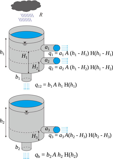
FIGURE 6. Conceptual sketch of tank model. The model has two tanks with an identical area A. Rainfall intensity (RI), given by R(t), is the water input source (h₁, h₂) are the tank water levels, (q₁, q₂, q₃) are discharge rates, and (q₁₂, q_b) are infiltration rates. Parameters (a₁, a₂, a₃) are discharge coefficients and (b₁, b₂) are infiltration coefficients. The initial values of (h₁, h₂) are denoted as (S₁, S₂) (not shown in the figure). The total water depth, h₁ + h₂ is referred to as the water storage index (WSI) in the present study. H (⋅) is the Heaviside function to ensure uni-directional water discharge and infiltration. In applications, A is the area of the catchment.

The lower tank in Figure 6 models the water flow and storage in the deep bedrock layer. The water storage of the lower tank is defined as h₂(t) and it has two discharge exits such that their discharges are q₃ = a₃A (h₂ − H₃)H (h₂ − H₃) and q_b = b₂Ah₂H (h₂). Similar to the upper tank counterpart, the governing equation for the lower tank is d h₂(t)/dt = (q₁₂ − q₃ − q_b)/A, with the initial value h₂ (T₀) = S₂. There are three additional constant parameters defined, a₃, b₂ and H₃, and their implications are the same as those of the upper counterpart. To summarize, there are two model equations to describe the water storage in each tank. The side outflows, q₁, q₂ and q₃, contribute to observable flow discharge and the discharge through the bottom-most exit, q_b, represents the discharge through an unobservable underground path. Therefore, the sum of the side exits is the volume flow rate discharged from the catchment. Rainfall in the model is the sole water input to the system.

The key triggering mechanism of landslides is the water content in slopes. During rainfall, the increase in water content increases the pore water pressure such that the effective stresses of slope materials decrease; hence, landslide motion is triggered. With the tank model, the water content in slopes is thought to be proportional to the total water storage of the two tanks, h₁ + h₂. Hence, we validate this assumption by inspecting the temporal correlation of the GPS surface displacement records with the water storage. This quantity, h₁ + h₂, is referred to as the WSI, and, we assume that it is proportional to the water content per unit area of the catchment.

To adapt the model to the present study areas, the model parameters must be calibrated. This calibration is achieved by minimizing the mean square error between the model discharge (the observable total side exit discharge) and the recorded volume flow rate. Mathematically, it reads

$F(\mathbf{p})=\frac{1}{T_f-T_0}\underset{\mathbf{p}}{\min }\left\{{\int }_{T_0}^{T_f}{(q_1+q_2+q_3-q_{\text{obs}})}^{2}dt\right\},$

where T₀, T_f are the initial and terminal time of the inspected period and p is the parameters to be calibrated. Symbol q_obs is the monitored volume flow rate that flows out of the catchment. In our study areas, q_obs was the volume flow rate measured at A-Chy-Ba Bridge for the TienChih catchment and at Hsin-Wu-Lu for the SiangYang catchment. Precaution must be taken because even though the present tank model is simplified from a standard three-tank model, there are still ten parameters to be calibrated. These parameters, represented by p in the above expression, include three discharge coefficients (a₁, a₂, a₃), two infiltration coefficients (b₁, b₂), three controlling threshold depths (H₁, H₂, H₃), and two initial water storage levels (S₁, S₂). The extensive number of parameters makes the calibration a ten-dimensional optimization process and can be computationally expensive. To improve the efficiency of calibration, a global optimization method called the shuffled complex evolution method (SCE-UA) is used to search the best set of parameters, Chen et al. (2013).

The SCE-UA method was developed in the 1990s, Duan et al. (1994), and has been widely applied to many hydrological-related studies, for example, characterization of catchment properties by Nasonova et al. (2009), Funke (1999), and Rustanto et al. (2017); algorithmic and mathematical aspects of the method and similar aspects by Kuczera (1997), Singh and Bárdossy (2015) and Seong et al. (2015); and a comprehensive review of its adaptations by Rahnamay Naeini et al. (2019). The search for the global optimum is based on the concept of competitive evolution of clusters of parameter sets, and is intrinsically a combination of probabilistic and deterministic approaches. In the present calibration scheme, we use a simple least square error estimator for a better resolution of the peak discharge rates between the model and measurement. In the following sections, the calibration and temporal correlation analysis of the TienChih landslide will first be described in detail, and then, the correlation analysis of the SiangYang landslide will be presented.

With the simple phenomenological quantitative tank model, the following two sections show that promising results can be obtained. However, we need to point out a few important precautions that should be taken when utilizing hydrological models. First, the tank model is suitable in principle for small-to medium-sized catchments. According to Okada et al. (2001), the maximum catchment size is conservatively suggested to be 10 km², although occasional applications to large catchments have been seen, e.g., ∼ 600 km² in Chen et al. (2005). In this regard, the application of the model to the two areas is a somewhat exaggerated overextension. Under these circumstances, the spatial transports of surface runoff and underground water are omitted. Exaggerated applications simply arise because of the lack of field data. In the mountain ranges of the island, only a few rain gauges and flow metre are installed to monitor the catchments. Therefore, aggressive tradeoffs have been made among the model accuracy, complexity and acquisition of phenomenological information.

Second, we tested the parameter calibration using standard three-tank models but the improvements were negligibly marginal. A heteroscedastic maximum likelihood estimator [HMLE; Sorooshian (1981)], has also been tested with the calibration procedure but this scheme usually led to underestimation of the peak discharge rates. Last, WSI, as the sum of water storage in the tanks, is expected to correlate with the underground water level. Unfortunately, there is no underground water information available for the two presented sites. It remains to be answered in future studies whether underground water information can be adopted as an additional constraint for parameter calibration and what efficacy can be obtained by doing so.

4 Analysis for the TienChih Landslide

For the TienChih landslide, rainfall records are taken from the Nan-Tien-Chih rainfall station, and the flow rate of the Laonung River is measured at the A-Chyi-Ba Bridge station. The locations of the two hydrological stations can be found in Figure 2 (caption) and 1. The catchment area in the calibration process is 411 km².

A typical result of the optimized tank model is shown in Figure 7. The result is for the year 2009. The discharge contribution of each tank in the model to the river flow rate is plotted in Figure 8. The discharge from the top tank is responsible for the peak river flow rate immediately after each rainfall event while the discharge from the bottom tank contributes to the lagged recessing river discharge. This observation agrees with the physical interpretation of the role of the discharges in the tank model.

FIGURE 7

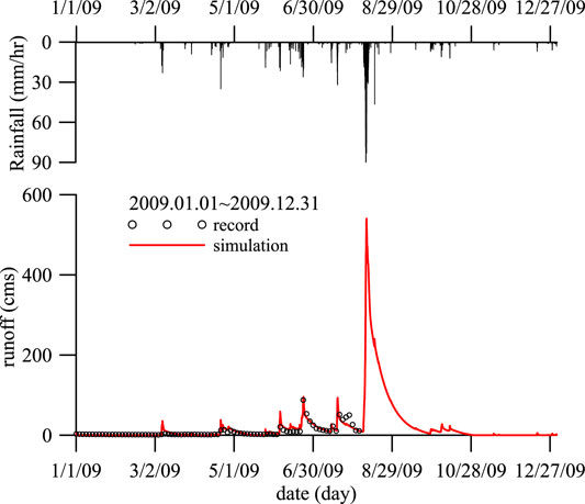
FIGURE 7. Calibrated river runoff volume flow rate of the TienChih catchment for 2009. The volume flow rate data were recorded by the A-Chyi-Ba Bridge station of the Laonung River. The measurement stopped on 8/9 because the instruments were destroyed by flooding.

FIGURE 8

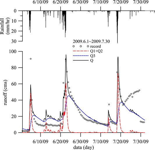
FIGURE 8. Comparison of volume flow rates from each tank. The volume flow rate data were recorded by the A-Chyi-Ba Bridge station of the Laonung River. The measurement data between 7/22 and 7/29 may contain instrumental errors but have negligible effects on the present annual calibration.

To streamline the analysis, we do not select any particular time series data for any individual landslide event. That is, the same procedure is applied annually to 2004, 2005, 2006 and 2009 (provided that 2009 has only 9 months of data). The optimized parameter sets for the years in which the TienChih GPS-recorded landslide motion is tabulated in Table 1. Because of the nonstationary regional climate system and inhomogeneous natural environment, there are variations among the four sets of model parameters. The unavoidable scarcity of data sources (one rainfall gauge and one flow station for each catchment) renders that model calibration suffers larger parameter variations among different sampling periods. Nevertheless, the results of a year-on-year comparison of the calibrated parameters are described as follows: 1) The discharge thresholds and initial water storage are on the orders of a unit magnitude, i.e., between 0 and a few tens, and 2) H₂ is close to zero. Figure 9 shows a simple sensitivity test for the model using the 2009 parameters for the 2006 data. The simple sensitivity test was performed to check if the characteristics of the river flow hydrograph remain. The hydrograph characteristics are the essential information for this model to work in the limit of present data scarcity. The sensitivity results show that the timing of peak river discharges is influenced very little, but the values of peak flow rates are underestimated in the case of the 2009 parameters. By inspecting the model sensitivity with other cases, we find that the variations in the peak flow rates are limited within an order of magnitude, or more specifically, within a maximum relative error of 300%. Therefore, caution must be used in regard to the parameter effects if the model parameters are not well calibrated. To illustrate the model sensibility further, we will reveal the result of the tank model with the 2009 mismatched parameter WSI-2009 in the following discussion.

TABLE 1

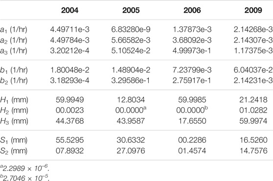
TABLE 1. Calibrated tank model parameters for the TienChih landslides.

FIGURE 9

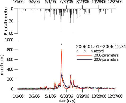
FIGURE 9. Calibrated river runoff volume flow rate of the TienChih catchment for 2006. The volume flow rate data were recorded by the A-Chyi-Ba Bridge station of the Laonung River. The volume flow rate prediction using the 2009 tank model parameters is also superposed for comparison.

Next, we inspect the relationship between the WSI and GPS-recorded surface displacement. For the four distinct landslide events, the related time series data, RI, WSI, and displacement, are sketched in Figure 10. Because of the poor weather conditions during rainfall, there were three events in 2004, 2005 and 2006 with intervals where the GPS signals were lost. Comparing the GPS data of these events prior to and after rainfall, it is likely that the landslides occurred within these GPS blind intervals. For all cases, landslides take place approximately when the WSIs reach maximum values and the landslides happened around 6/29/2004 (Month/Day/Year) Mindulle typhoon, 7/18/2005 Haitang typhoon, 5/17/2006 heavy rainfall and 8/7/2009 Morakot typhoon. Note that we neglect the GPS displacement fluctuations although there are occasions that the fluctuations somewhat follow the WSI alternations. It is because the fluctuations did not cause permanent displacements after the associated WSI events.

FIGURE 10

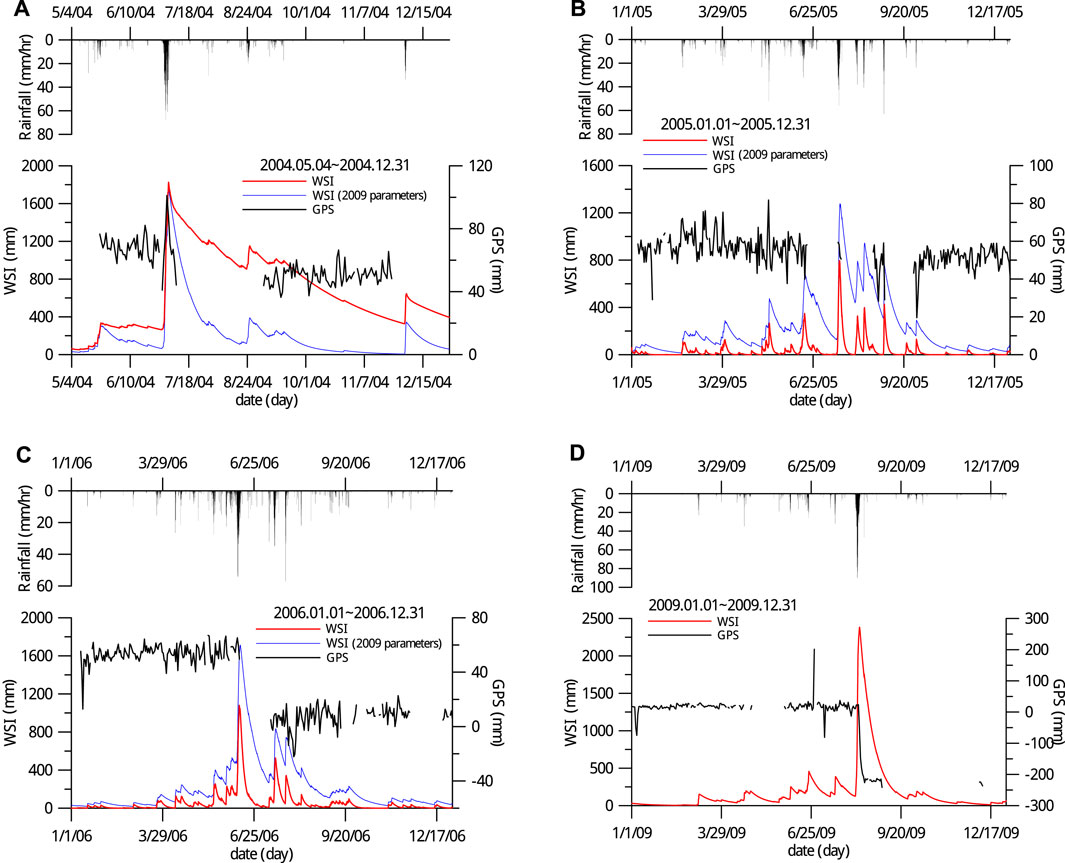
FIGURE 10. RI, WSI and GPS displacement of the four landslide events. WSI-2009 curves are WSI predictions using 2009 tank model parameters and they are superimposed for a model sensitivity check. The light blue shaded lines are landslide thresholds: between 350 ∼400 mm for WSI and approximately 40 mm/h for rainfall intensity. The associated landslide events from panels (A–D) are 6/29/2004 (Month/Day/Year) Mindulle typhoon, 7/18/2005 Haitang typhoon, 5/17/2006 heavy rainfall and 8/7/2009 Morakot typhoon.

Notably, the WSI in 2004 had a much longer water recession period which means a much lower discharge rate than the others. This difference occurs because the second tank has very low discharging rates (a₃ and b₂) after calibration for this year. Without other available auxiliary measurement data to verify this WSI estimation, we need to be cautious when interpreting its implications or adopting the model towards regional mitigation systems. For simplicity, we neglect the effects of the water recess periods but address the rising WSI on the landslide motion. A straightforward visual inspection suggests that the triggering threshold of the landslide motion is approximately WSI = 350 ∼ 400 mm, as indicated by the light-blue shaded marks in Figure 10. The main criterion is to fit the WSI and all of the four aforementioned landslides: the higher bound of the threshold range is about the lowest possible value that the landslide occurs; and the lower bound is about the highest possible value that the landslide does not occur. The WSI-2009 curves are also superposed with their corresponding events for sensitivity comparison, and the same threshold is applicable. A similar RI threshold can be obtained, and the threshold is approximately 40 mm/h. However, based on the RI, the 6/19/2005 event is not detected, as shown in Figure 10B, because precipitation duration is not properly weighted in this approach.

We have to keep in mind that the WSI threshold should be treated as a suggested level and is in general site dependent. It is because the determination of the threshold is by a simple and subjective comparison between the historical landslide events and WSI hydrograph, on the assumption that the WSI in slopes is directly associated with the variations of the material strengths without time lags. The threshold may be different if the model detail or monitoring network is changed. The accuracy of the threshold is also hard to assess in the present conditions because the number of the verified landslides does not reach a level of statistical significance. In addition, we also neglected the possibility that the threshold may change after each landslide because its change may involve subtle changes in geological conditions and they are not quantifiable in the current framework. Nevertheless, we illustrated the possibility to construct a WSI threshold for a landslide site from the aspects of presented model and data.

Most of the mainstream mitigation warning systems are based on regional statistical regression analyses using rainfall data, for example the peak RI, and duration. In this type of model, the infiltration of precipitation is usually neglected. With the present tank model, infiltration can be taken into consideration. Therefore for comparison, we evaluate the predictions between the RI and WSI approaches. We use the 2009 event for this assessment because it has a continuous displacement record to cover the entire motion. We assume that the rate of displacement is proportional to the water storage, i.e., WSI in the slope because water directly reduces the strengths of the materials; thus, it is expected that the displacement rate (DR) is synchronized with the WSI. To investigate this assumption, we apply a correlation function to calculate the phase difference, or time-lag, between the WSI and DR. The correlation function is defined as follows: as

$\text{corr}(\text{DR},\text{WSI})=\text{E}(\text{DR}(t)\cdot \text{WSI}(t+\tau )),$

which is the expectancy value, E (⋅), of the product of the DR and a time-τ-shifted WSI. For comparison, the correlation functions between the DR, first tank water depth h₁ and RI are also calculated by replacing WSI in the above expression with R(t) and h₁(t). In the calculation, we use 1-month time series data starting from 7/28/2009 and the close-up time series, including RI, displacement, DR, h₁ and WSI are shown in Figure 11.

FIGURE 11

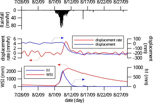
FIGURE 11. Close-up time series plots of the 2009 Morakot typhoon triggered TienChih landslide. From the top panel: RI; middle: displacement, DR; bottom: h₁ and WSI. The DR is the negated time derivative of the GPS displacement.

The three correlation functions are plotted in Figure 12. In the plot, the maximum values of the correlation functions indicate the similarities in shapes and timescales of the correlated signals and their corresponding time shifts imply time lags between the correlated signals. From the time shift, we find that the peak of the WSI correlation function occurs at approximately 13 h while those of h₁ and RI correlation functions are at − 22 and −34 h. The negative time shifts indicate that h_i and RI events temporally occur prior to the DR. The alternation of the time shifts, from RI, h₁ to WSI, reveals the role of water infiltration to the landslide. The timing sequentially approaches the landslide displacement from the precursor rainfall, water accumulation in the shallow surface layer, and to the deep layer. This sequence confirms not only the assumption that the peak DR occurs closer to the predicted peak of WSI than h₁ and RI but also the phenomenological fact of the tank model that the deep-seated landslide involves water in the deep bed rock layer. Last, because of the water infiltration mechanism, the WSI has a much longer water recession period than rainfall, and subsequently, this recession period results in a lowering and broadening peak of the correlation function.

FIGURE 12

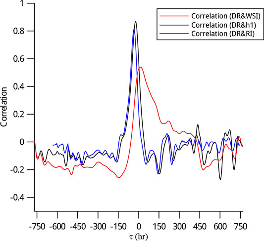
FIGURE 12. Correlation functions. One month time series data from 7/28/2009 are used for calculation. The negative time shift (negative τ) represents the time lead to the DR. The large horizontal time lag axis is chosen for clearer visual inspection of the correlation functions.

5 The SiangYang Landslide Case

The SiangYang landslide was triggered by the 2009 Morakot typhoon. By using the same technique described in Section 3, the tank model parameters for 2009 are computed and listed in Table 2. The calibrated runoff hydrograph compared with the monitoring data of the Hsin-Wu-Lu River flow station is shown in Figure 13. To investigate the occurrence sequence of the landslide more precisely, close-up hydrographs of the RI, displacement, DR, h₁ and WSI are plotted in Figure 14. Comparing the calibrated parameters to those of the 2009 TienChih catchment, the discharge coefficients, a_1,3, are roughly an order of magnitude larger (10×), indicating that the region has a higher water mobility, i.e., lower water retention (holding) capacity. Consequently, the discharge recession period is short and the hydrological characteristics of the catchment are dominated by those of the first tank. Verification is shown by the fact that the WSI is almost identical to h₁, as shown in the bottom panel of Figure 14. The same WSI threshold in the TienChih landslide (350 ∼400 mm) is also found applicable to the SiangYang landslide. However, we cannot yet conclude if the threshold fits tightly to the landslide initiation under the present scope of data. The constraints of the threshold discussed in Section 4 still hold to the SiangYang site. Under this circumstance, we should treat the threshold conservatively as a necessary but not a sufficient condition for triggering the SiangYang landslide motion. Nevertheless, the coincidence of the threshold in both the SiangYang and TienChih landslide sites may imply that it may be insensitive to a wide range of geological conditions. This implication is important for applications of the technique and Whether it is true remains open for future research.

TABLE 2

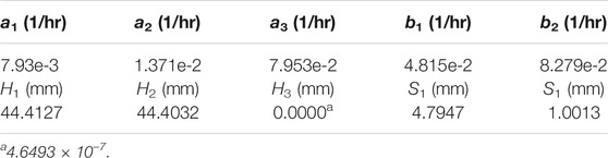
TABLE 2. Calibrated tank model parameters for the 2009 SiangYang landslide.

FIGURE 13

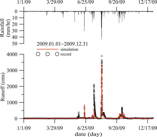
FIGURE 13. Calibrated river runoff volume flow rate of the SiangYang catchment for 2009. The volume flow rate data were recorded by the Hsin-Wu-Lu river flow station of the Beinan River.

FIGURE 14

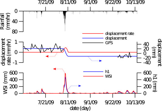
FIGURE 14. Close-up time series plots of the 2009 Morakot rainfall-triggered SiangYang landslide. From the top panel: RI; middle: displacement, DR; bottom: h₁ and WSI. The DR is the negated time derivative of the GPS displacement. The light blue shaded line in the bottom panel indicates the WSI threshold inferred in the TienChih landslide.

Similar to the TienChih case, the time series of the GPS displacement-related data are also missing for approximately one and a half months after the Morakot typhoon, as shown in the middle panel of Figure 14. To proceed with the calculation of the temporal correlation functions, we assume that the slope starts to move immediately after the time when the GPS data are missing, i.e., on September 8, 2009, and the motion lasts for approximately 5 days by referring to the TienChih landslide, cf. Figure 11. Over the 5-day duration, the area catches most of the precipitation from the Morakot typhoon. Under this assumption, we use two constant position values and a smooth sinusoidal function to synthesize the landslide displacement, which is a quarter wave length sinusoidal function with both ends joining the constants on its both sides, as shown by the blue line in the middle panel of Figure 14. The constant position values are the average position of the GPS station before and after the landslide. Based on the synthesized displacement, the DR is calculated, as shown by the red line in the same figure panel. Because the displacement of the SiangYang landslide is only approximately one-tenth of that in the TienChih case, the GPS displacement data have a low signal-to-noise ratio. To avoid employing further sophisticated signal processing techniques, we use the synthesized displacement for the temporal correlation analysis. Similar to Section 4, 1-month time series data starting from 7/28/2009 are used in the calculation.

The correlation functions for the SiangYang landslide are calculated and presented in Figure 15. Our attention is drawn to the time shifts between the hydrological variables and DR, which are −4.7, −6.3 and −19 h for the WSI, h₁ and RI, respectively. All negative time shift values indicate that the hydrological hydrographs are ahead of the DR. The alternation of the time shifts follows the same order we observed in the previous section, from RI, h₁ to WSI, revealing the local water cycle movement. Similar to the TienChih landslide, the DR is closest to the WSI hydrograph, implying that the landslide involves water in the deep layer. Because the hydrological characteristics of the site are primarily dependent on the first tank, the WSI and h₁ correlation functions are also nearly identical and their time difference is only approximately 1.6 h. Finally for this case, some artefacts have been introduced into the correlation functions because of the use of the synthesized displacement. These effects include the noise-free well-defined shape of the function and the nearly perfect correlation ($\approx 0.9$) at the function peak.

FIGURE 15

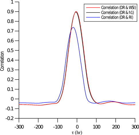
FIGURE 15. Correlation functions. One-month time series data from 7/28/2009 are used for calculation. The negative time shift (negative τ) represents the time lead to the DR. The large horizontal time lag axis is chosen for clearer visual inspection of the correlation functions.

6 Discussion

Our attention was drawn to the temporal correlation between the creeping landslide motion and water content in slopes. The TienChih and SiangYang landslides were chosen because they are rainfall-triggered, deep-seated creeping landslides, and their locations are in the upstream-most catchment areas. Because of the accessibility of the sites and the associated mountain range, field measurements for calibrating sophisticated field models are scarce. As a trade-off, we adopted a phenomenological quantitative hydrological model, the simplified tank model, to model the local water cycles.

The water storage in the solid slope was assumed to be proportional to the sum of the water depths of the two serially-connected tanks, h₁ + h₂, which is referred to as the WSI. In the classical literature of the model, the WSI is called the soil water index, or SWI. We deliberately avoided using the term because it is intuitively associated with shallow soil-based debris landslides. By virtue of the phenomenological tank model, no restrictions are imposed on the material types, detailed distribution configuration of the materials, or physical dimension of the slopes. These physical and geological effects are indirectly incorporated into the parameters of the model through the parameter calibration processes.

Because of the active tectonic motion Lee and Wang (1985) and Lai et al. (1989), rich networks of fracture and cleavage structures are developed in the mountain bedrock. Borehole investigations and rock core samples in the neibouring area with similar geological conditions reveal that fractured geostructures persist at least to one hundred metre from the surface Lin and Lin (1999); Chinese American Tech. Corp. et al. (1992). Therefore, it is assumed that water can infiltrate deeply into bedrock through these open disjointed networks during heavy rainfall periods. As a result, water accumulation in the slope lifts the groundwater table, leading to an increase in the pore pressure, a reduction in the effective stresses and consequently triggering landslide motion. Based on this hypothesis, the occurrence of landslide motion is expected to correlate closely with the WSI and has been verified with the two presented landslides.

In the tank model, the arrangement of the side water exits is conceptually associated with the discharges from the surface runoff, surface and deep bedrock (or subsoil) layers according to Sugawara (1995). In this arrangement, H₁ must be higher than H₂, as shown by the calibrated parameters of the two presented catchments, Tables 1, 2. Having confirmed the configuration of the discharge exits of the first tank, it is noticed that the discharge coefficient of the top-most exit, a₁, is smaller overall than a₂. This result implies that the discharge of the first tank is primarily controlled by the surface layer, i.e., the discharge through the lower a₂ exit.

Comparing the 2009 calibration results, we find that the two sets of parameters lead to one distinct difference in the local water cycles. The TienChih catchment has a smaller b₂, such that it keeps water above the second tank for a longer period and causes a longer recession period of the flow rate of the Laonung River. In contrast, the SiangYang catchment has a larger infiltration capability such that water can quickly infiltrate through the second tank into the deeper bedrock layer. Despite the aforementioned distinct hydrological characteristics, the WSI threshold of 350 ∼400 mm is applicable for both landslides.

7 Conclusion

In this paper, the rainfall-triggered TienChih and SiangYang deep-seated creeping landslides were compared with the regional water cycles. The landslide displacement motion was recorded by continuous GPS stations, and the regional water cycles included hydrological variables, such as precipitation, water storage in the catchment and runoff flow. The aim of this study is to illustrate that the infiltration of surface water and water storage in the catchment were associated with landslide motion. The water cycles were modelled using the phenomenological tank model, which was composed of two serially-connected tanks. The model contained a total of ten parameters to be calibrated against the rainfall and river runoff flows. The water content in the catchments, i.e., on the solid slopes, was quantified by using the water depth of the first tank (h₁) and the total water depth, (WSI, h₁ + h₂).

The association between landslide motion and water cycles was investigated by their correlations. The correlation functions, and thus the time lags, between the DR and the hydrological variables (RI, h₁ and WSI) were calculated. Comparing the time lags, we found that the RI lead ahead, followed by h₁, and finally, the WSI correlated the closest in time to landslide motion. This sequence clearly indicated the infiltration processes where the water was transported from the surface, through the shallow soil layer, and into the deep bedrock layer. When a certain depth was reached, the water weakened the slope material and triggered landslide motion. Therefore, we can expect that the WSI and landslide motion correlates the best in time but not their appearing order because the detail underground water flows and material weakening mechanism were not modelled. On the direct relationship between the WSI and landslide motion, we suggested a WSI threshold for the investigated deep-seated landslides that was between 350 and 400 mm. The same WSI threshold is applicable to both landslides lead to an important implication that it may be insensitive to a wide range of geological conditions. This proposition needs to be carefully examined with more landslide cases in future. To summarize, the hydrological technique presented in the paper provides the interrelation among the hydrological variables, and in turn, the WSI hydrograph and its threshold can act as valuable accessorial quantities that are beneficial to accurately estimating deep-seated landslide initiation in future hazard mitigation warning system.

Data Availability Statement

The raw data supporting the conclusion of this article will be made available by the authors, without undue reservation.

Author Contributions

C-YK, R-FC and Y-JH contributed to conception and design of the study. C-YK, S-EL and Y-HC developed and executed the hydrological model. S-PL, R-FC and Y-JH provided GPS and hydrological data. C-WL, K-JC and R-YW provided geological investigation details. All authors contributed to manuscript revision, read, and approved the submitted version.

Funding

This work is supported in parts by the Bureau of Soil Water Conservation, Taiwan, under grants SWCB-105-128 and SWCB-110-028.

Conflict of Interest

The authors declare that the research was conducted in the absence of any commercial or financial relationships that could be construed as a potential conflict of interest.

Publisher’s Note

All claims expressed in this article are solely those of the authors and do not necessarily represent those of their affiliated organizations, or those of the publisher, the editors and the reviewers. Any product that may be evaluated in this article, or claim that may be made by its manufacturer, is not guaranteed or endorsed by the publisher.

References

Altamimi, Z., Collilieux, X., Legrand, J., Garayt, B., and Boucher, C. (2007). ITRF2005: a New Release of the International Terrestrial Reference Frame Based on Time Series of Station Positions and Earth Orientation Parameters. J. Geophys. Res. 112, B09401. doi:10.1029/2007jb004949

CrossRef Full Text | Google Scholar

Cappa, F., Guglielmi, Y., Soukatchoff, V. M., Mudry, J., Bertrand, C., and Charmoille, A. (2004). Hydromechanical Modeling of a Large Moving Rock Slope Inferred from Slope Levelling Coupled to spring Long-Term Hydrochemical Monitoring: Example of the La Clapière Landslide (Southern Alps, France). J. Hydrol. 291, 67–90. doi:10.1016/j.jhydrol.2003.12.013

CrossRef Full Text | Google Scholar

Chen, R.-F., Hsu, Y.-J., Yu, S.-B., Chang, K.-J., Wu, R.-Y., Hsieh, Y.-C., et al. (2015). “Real-time Monitoring of Deep-Seated Gravitational Slope Deformation in the Taiwan Mountain Belt,” in Engineering Geology for Society and Territory - Volume 2. Editors G. Lollino, D. Giordan, G. B. Crosta, J. Corominas, R. Azzam, J. Wasowskiet al. (Berlin, Germany: Springer), 1333–1336. doi:10.1007/978-3-319-09057-3_234

CrossRef Full Text | Google Scholar

Chen, R.-S., Pi, L.-C., and Hsieh, C.-C. (2005). Application of Parameter Optimization Method for Calibrating Tank Model. J. Am. Water Resour. Assoc. 41, 389–402. doi:10.1111/j.1752-1688.2005.tb03743.x

CrossRef Full Text | Google Scholar

Chen, S. C., Tsai, C. W., Chen, C. Y., and Chen, M. C. (2013). Soil Water index Applied as a Debris Flow Warning-Reference Based on a Tank Model. J. Chin. Soil Water Conserv. 44, 133–143. doi:10.29417/JCSWC.201306_44(2).0004

CrossRef Full Text | Google Scholar

Chinese American Tech. Corp.China Eng. Consult. Inc.Atci Corp. (1992). Preliminary Planning and Feasibility Study of the National South Transverse Highway (In Chinese). Taiwan: Taiwan Area National Expressway Engineering Bureau, Ministry of Transportation and Communications.

Google Scholar

Duan, Q., Sorooshian, S., and Gupta, V. K. (1994). Optimal Use of the SCE-UA Global Optimization Method for Calibrating Watershed Models. J. Hydrol. 158, 265–284. doi:10.1016/0022-1694(94)90057-4

CrossRef Full Text | Google Scholar

Funke, R. (1999). Parameterization and Regionalization of a Runoff Generation Model for Heterogeneous Catchments. Phys. Chem. Earth, B: Hydrol. Oceans Atmosphere 24, 49–54. doi:10.1016/S1464-1909(98)00010-0

CrossRef Full Text | Google Scholar

Herring, T. A., King, R. W., and McClusky, S. C. (2002). Documentation for the GAMIT Analysis Software, Release 10.0 Edn. Cambridge, MA: MIT.

Google Scholar

Hsu, Y.-J., Chen, R.-F., Lin, C.-W., Chen, H.-Y., and Yu, S.-B. (2014). Seasonal, Long-Term, and Short-Term Deformation in the Central Range of Taiwan Induced by Landslides. Geology 42, 991–994. doi:10.1130/G35991.1

CrossRef Full Text | Google Scholar

Ishihara, Y., and Kobatake, S. (1979). Runoff Model for Flood Forecasting. Bull. Disaster Prev. Res. Inst. Kyoto Univ. 29, 27–43.

Google Scholar

Kuczera, G. (1997). Efficient Subspace Probabilistic Parameter Optimization for Catchment Models. Water Resour. Res. 33, 177–185. doi:10.1029/96WR02671

CrossRef Full Text | Google Scholar

Lai, T. C., Aj, K. F., Chen, F. C., Fei, L. W., and Liu, H. T. (1989). Geological Survey and Study on the Potential Dangers in the Guanshan Area of Yushan National Park (In Chinese). Tech. Rep., Yushan National Park Trans., No. 1017.

Google Scholar

Lee, C. T., and Wang, Y. (1985). Stratigraphy and Structure of the Slate Terrane Near Likuan Southern Cross-Island Highway, Taiwan (In Chinese). Ti-Chi 8, 1–20.

Google Scholar

Lee, K. T. (1993). Tank Model and Rainfall-Runoff Simulation. J. Chin. Agric. Eng. 39 (2), 20–28.

Google Scholar

Lin, C. C., and Lin, C. C. (1999). Engineering Geological Servey and Treatment Planning Study at 191k+772 Chiabao Tunnel, South Transverse Highway (In Chinese). Taiwan Highw. Eng. 25, 24–38.

Google Scholar

Lin, C. W. (2012). Geological Environment Monitoring and Facilities Safety Assessment of Yushan National Park (In Chinese). Tech. Rep., Yushan National Park Trans., No. 1254.

Google Scholar

Lin, S. E., Chan, Y. H., Kuo, C. Y., Chen, R. F., Hsu, Y. J., Chang, K. J., et al. (2017). The Use of a Hydrological Catchment Model to Determine the Occurrence of Temporal Creeping in Deep-Seated Landslides. J. Chin. Soil Water Conserv. (in Chinese) 48, 153–162. doi:10.29417/JCSWC.201712_48(4).0001

CrossRef Full Text | Google Scholar

Liu, J. D., Doan, C. D., and Liong, S. Y. (2010). “Conceptual Rainfall-Runoff Model with Kalman Filter for Parameter and Outflow Updating,” in Advances in Geosciences, Volume 23: Hydrological Science. Editor G. F. Lin (Singapore: World Sci. Pub.), 133–146.

Google Scholar

Lv, H., Ling, C., Hu, B. X., Ran, J., Zheng, Y., Xu, Q., et al. (2019). Characterizing Groundwater Flow in a Translational Rock Landslide of Southwestern China. Bull. Eng. Geol. Environ. 78, 1989–2007. doi:10.1007/s10064-017-1212-3

CrossRef Full Text | Google Scholar

Nasonova, O. N., Gusev, Y. M., and Kovalev, Y. E. (2009). Investigating the Ability of a Land Surface Model to Simulate Streamflow with the Accuracy of Hydrological Models: A Case Study Using MOPEX Materials. J. Hydrometeorology 10, 1128–1150. doi:10.1175/2009JHM1083.1

CrossRef Full Text | Google Scholar

Nie, W., Krautblatter, M., Leith, K., Thuro, K., and Festl, J. (2017). A Modified Tank Model Including Snowmelt and Infiltration Time Lags for Deep-Seated Landslides in alpine Environments (Aggenalm, germany). Nat. Hazards Earth Syst. Sci. 17, 1595–1610. doi:10.5194/nhess-17-1595-2017

CrossRef Full Text | Google Scholar

Okada, K., Makihara, Y., Shimpo, A., Nagata, K., Kunitsugu, M., and Saitoh, K. (2001). Soil water index (SWI) (in Japanese). Tenki 48, 349–356.

Google Scholar

Osanai, N., Shimizu, T., Kuramoto, K., Kojima, S., and Noro, T. (2010). Japanese Early-Warning for Debris Flows and Slope Failures Using Rainfall Indices with Radial Basis Function Network. Landslides 7, 325–338. doi:10.1007/s10346-010-0229-5

CrossRef Full Text | Google Scholar

Padilla, C., Onda, Y., Iida, T., Takahashi, S., and Uchida, T. (2014). Characterization of the Groundwater Response to Rainfall on a Hillslope with Fractured Bedrock by Creep Deformation and its Implication for the Generation of Deep-Seated Landslides on Mt. Wanitsuka, Kyushu Island. Geomorphology 204, 444–458. doi:10.1016/j.geomorph.2013.08.024

CrossRef Full Text | Google Scholar

Rahnamay Naeini, M., Analui, B., Gupta, H. V., Duan, Q., and Sorooshian, S. (2019). Three Decades of the Shuffled Complex Evolution (Sce-ua) Optimization Algorithm: Review and Applications. Scientia Iranica 26, 2015–2031. doi:10.24200/sci.2019.21500

CrossRef Full Text | Google Scholar

Rustanto, A., Booij, M. J., Wösten, H., and Hoekstra, A. Y. (2017). Application and Recalibration of Soil Water Retention Pedotransfer Functions in a Tropical Upstream Catchment: Case Study in Bengawan Solo, indonesia. J. Hydrol. Hydromechanics 65, 307–320. doi:10.1515/johh-2017-0020

CrossRef Full Text | Google Scholar

Seong, C., Her, Y., and Benham, B. (2015). Automatic Calibration Tool for Hydrologic Simulation Program-Fortran Using a Shuffled Complex Evolution Algorithm. Water 7, 503–527. doi:10.3390/w7020503

CrossRef Full Text | Google Scholar

Singh, S., and Bárdossy, A. (2015). Hydrological Model Calibration by Sequential Replacement of Weak Parameter Sets Using Depth Function. Hydrology 2, 69–92. doi:10.3390/hydrology2020069

CrossRef Full Text | Google Scholar

Sorooshian, S. (1981). Parameter Estimation of Rainfall-Runoff Models with Heteroscedastic Streamflow Errors - the Noninformative Data Case. J. Hydrol. 52, 127–138. doi:10.1016/0022-1694(81)90099-8

CrossRef Full Text | Google Scholar

Sugawara, M. (1995). “Chapter 6, Tank Model,” in Computer Models for Watershed Hydrology. Editor V. P. Singh (Littleton, Colo: Water Res. Pub.).

Google Scholar

Sugawara, M., and Funiyuki, M. (1956). “A Method of Revision of the River Discharge by Means of a Rainfall Model,” in Collection of Research Papers about Forecasting Hydrologic Variables (Saitama, Japan: Geosphere Res. Institute of Saitama Univ.), 14–18.

Google Scholar

Sugawara, M. (1961). On the Analysis of Runoff Structure about Several Japanese Rivers. Jpn. J. Geophys. 2 (4), 210–216.

Google Scholar

Takahashi, K., Ohnishi, Y., Xiong, J., and Koyama, T. (2008). Tank Model and its Application to Predicting Groundwater Table in Slope. Chin. J. Rock Mech. Eng. 27 (12), 2501–2508.

Google Scholar

Varnes, D. J. (1978). “Slope Movement Types and Processes,” in Special Report 176: Landslides: Analysis and Control. Editors R. L. Schuster, and R. J. Krizek (Washington D. C.: Transportation and Road Research Board, Natl. Acad. Sci.), 11–33.

Google Scholar

Yokoo, Y., Kazama, S., Sawamoto, M., and Nishimura, H. (2001). Regionalization of Lumped Water Balance Model Parameters Based on Multiple Regression. J. Hydrol. 246, 209–222. doi:10.1016/s0022-1694(01)00372-9

CrossRef Full Text | Google Scholar

Yu, S.-B., Chen, H.-Y., and Kuo, L.-C. (1997). Velocity Field of GPS Stations in the Taiwan Area. Tectonophysics 274, 41–59. doi:10.1016/s0040-1951(96)00297-1

CrossRef Full Text | Google Scholar

Yu, S.-B., Hsu, Y. J., Kuo, L. C., Chen, H. Y., and Liu, C. C. (2003). GPS Measurement of Postseismic Deformation Following the 1999 Chi-Chi, Taiwan, Earthquake. J. Geophys. Res. 108, 2520. doi:10.1029/2003jb002396

CrossRef Full Text | Google Scholar

Zêzere, J. L., Trigo, R. M., and Trigo, I. F. (2005). Shallow and Deep Landslides Induced by Rainfall in the lisbon Region (Portugal): Assessment of Relationships with the North Atlantic Oscillation. Nat. Hazards Earth Syst. Sci. 5, 331–344. doi:10.5194/nhess-5-331-2005

CrossRef Full Text | Google Scholar