Ensemble-Based Forecast of Volcanic Clouds Using FALL3D-8.1

Operational forecasting of volcanic ash and SO₂ clouds is challenging due to the large uncertainties that typically exist on the eruption source term and the mass removal mechanisms occurring downwind. Current operational forecast systems build on single-run deterministic scenarios that do not account for model input uncertainties and their propagation in time during transport. An ensemble-based forecast strategy has been implemented in the FALL3D-8.1 atmospheric dispersal model to configure, execute, and post-process an arbitrary number of ensemble members in a parallel workflow. In addition to intra-member model domain decomposition, a set of inter-member communicators defines a higher level of code parallelism to enable future incorporation of model data assimilation cycles. Two types of standard products are automatically generated by the ensemble post-process task. On one hand, deterministic forecast products result from some combination of the ensemble members (e.g., ensemble mean, ensemble median, etc.) with an associated quantification of forecast uncertainty given by the ensemble spread. On the other hand, probabilistic products can also be built based on the percentage of members that verify a certain threshold condition. The novel aspect of FALL3D-8.1 is the automatisation of the ensemble-based workflow, including an eventual model validation. To this purpose, novel categorical forecast diagnostic metrics, originally defined in deterministic forecast contexts, are generalised here to probabilistic forecasts in order to have a unique set of skill scores valid to both deterministic and probabilistic forecast contexts. Ensemble-based deterministic and probabilistic approaches are compared using different types of observation datasets (satellite cloud detection and retrieval and deposit thickness observations) for the July 2018 Ambae eruption in the Vanuatu archipelago and the April 2015 Calbuco eruption in Chile. Both ensemble-based approaches outperform single-run simulations in all categorical metrics but no clear conclusion can be extracted on which is the best option between these two.

1 Introduction

Numerical modelling of volcanic plumes, including the atmospheric dispersal of volcanic particles and aerosols and its ultimate fallout on the ground, is challenging due to a number of reasons that include, among others, the multiplicity of scales involved, the complex underlying physical phenomena, the characterisation of the emitted particles and aerosols, and the quantification of the strength, vertical distribution, and evolution in time of the source term (volcanic plume) and related uncertainties (Folch, 2012). The latter two aspects are particularly critical in operational forecast scenarios where, in addition to larger source term uncertainties, requirements exist also on the forecast time-to-solution that constrain the space-time resolutions of operational model setups depending on the computational resources available.

Ensemble-based modelling is well recognised as the proper strategy to characterise uncertainties in model inputs, in model physics and its parameterisations, and in the underlying model-driving meteorological data. In the fields of meteorology and atmospheric dispersal, the use of ensemble-based approaches to improve predictions and quantify model-related uncertainties has long been considered, first in the context of numerical weather forecast (e.g., Mureau et al., 1993; Bauer et al., 2015), and afterwards for toxic dispersal (e.g., Dabberdt and Miller, 2000; Maurer et al., 2021), air quality (e.g., Galmarini et al., 2004; Galmarini et al., 2010), or volcanic clouds (e.g., Bonadonna et al., 2012; Madankan et al., 2014; Stefanescu et al., 2014) among others. Ensemble-based approaches can give a deterministic product based on some combination of the single ensemble members (e.g., the ensemble mean) and, as opposed to single deterministic runs, attach to it an objective quantification of the forecast uncertainty. On the other hand, ensemble runs can also furnish probabilistic products based on the fraction of ensemble members that verify a certain (threshold) condition, e.g., the probability of cloud being detected by satellite-based instrumentation, the probability that the cloud mass concentration compromises the safety of air navigation, the probability of particle fallout or of aerosol concentration at surface to exceed regulatory values for impacts on infrastructures or on air quality, etc. Added to these, ensembles can also be used as multiple trial simulations, e.g., in optimal source term inversions by calculating correlations between the different members and observations (e.g., Zidikheri et al., 2017; Zidikheri et al., 2018; Harvey et al., 2020) or to make more robust in flight-planning decisions (Prata et al., 2019). Finally, ensembles are also the backbone of most modern data assimilation techniques, which require estimates of forecast uncertainty to merge a priori forecasts with observations during data assimilation cycles (e.g., Fu et al., 2015; Fu et al., 2017; Osores et al., 2020; Pardini et al., 2020).

At a research level, forecasting of volcanic clouds using ensemble-based approaches has been considered in several models including, for example, ASH3D (Denlinger et al., 2012a; Denlinger et al., 2012b), COSMO-ART (Vogel et al., 2014), HYSPLIT (Dare et al., 2016; Zidikheri et al., 2018; Pardini et al., 2020), NAME (Dacre and Harvey, 2018; Beckett et al., 2020), FALL3D (Osores et al., 2020) or, more recently, even tackling multi-model ensemble approaches (Plu et al., 2021). Despite promising results, implementations at operational level are still limited to a few cases, e.g. the Dispersion Ensemble Prediction System (DEPS) of the Australian Bureau of Meteorology (Dare et al., 2016). Such a slow progress can be explained by the inertia of operational frameworks to go beyond single-run scenarios, the limited pool of validation studies supporting this approach, the computational overhead of ensemble-based forecast methodologies, the reluctance of some end-users to incorporate probabilistic scenarios in their decision-making operations, or even the difficulties to interpret and communicate ensemble-based products. Here we present FALL3D-8.1, the last version release of this atmospheric transport model that includes the option of ensemble-based simulations. Developments are being done in the frame of the EU Center of Excellence for Exascale in Solid Earth (ChEESE) and, more precisely, within the Pilot Demonstrator (PD) number 12 (PD12) that considers an ensemble-based data assimilation workflow combining the FALL3D dispersal model with high-resolution latest-generation geostationary satellite retrievals. The ultimate goal of this pilot is to have a km-resolution short and long-range automated forecast system with edge-to-end latencies compatible with early-warning and crisis management requirements. We limit our discussion here to the ensemble modelling module, leaving the data assimilation component to another publication linked to the upcoming v8.2 model release (Mingari et al., 2021). In this scenario, the objectives of this manuscript are three-fold:

1. To introduce FALL3D-8.1, including the novel model tasks to generate ensemble members from an unperturbed reference member, merge and post-process the single-member simulations, and validate model forecasts against satellite-based and ground deposit observations (Section 2). The ensemble generation in FALL3D-8.1 can consider uncertainties in the emissions (i.e., the so-called Eruption Source Parameters for volcanic species), particle properties, and meteorological fields (wind velocity).

2. To define quantitative forecast-skill metrics applicable to both ensemble-based deterministic and ensemble-based probabilistic forecasts simultaneously. Note that, typically, only ensemble-based deterministic outputs are compared against observations, e.g., by means of categorical metrics. However, the question on whether a probabilistic approach is more (or less) skilled than a deterministic one is rarely tackled. Generalised categorical metrics are proposed in Section 3 of this paper in order to explicitly address this question.

3. To validate the ensemble-based deterministic and probabilistic approaches using different types of observation datasets for ash/SO₂ clouds (satellite detection and satellite retrieval) and ground deposits (scattered points and isopach contours). This is done in two different contexts, the July 2018 Ambae eruption for SO₂ clouds, and the April 2015 Calbuco eruption for ash clouds and tephra fallout (Section 4). In both cases, computational capacity requirements are considered in the context of urgent (super)-computing, including constraints in the forecast time-to-solution.

2 FALL3D-8.1

During its latest major version release (v8.0), the FALL3D model (Costa et al., 2006; Folch et al., 2009) was rewritten and refactored in order to incorporate dramatic improvements in model physics, spectrum of applications, numerics, code scalability, and overall code performance on large supercomputers (for details see Folch et al., 2020; Prata et al., 2021). This included also the parallelisation and embedding of former pre-process auxiliary programmes to run either as independent model tasks (specified by a call argument) or concatenated in a single execution workflow. In FALL3D-8.1, three new model tasks have been added to automatically generate an ensemble of members (task SetEns), post-process ensemble-based simulations (task PosEns) and, finally, validate the model against different types of observation datasets (task PosVal). Ensemble members in FALL3D-8.1 run concurrently in parallel, with a dedicated MPI communicator for the master ranks of each ensemble member. However, because this code version does not handle data assimilation cycles yet (something planned for the next version release v8.2), the individual ensemble members run actually as an embarrassingly parallel workload (e.g., Herlihy et al., 2020), i.e., with no dependency among parallel tasks.

2.1 Ensemble Generation Task

The task SetEns, which must be run first in the case of ensemble runs, generates and sets the ensemble members from a unique input file by perturbing a reference case (the so-called central or reference member). This task also creates a structure of sub-folders, one for each ensemble member, where successive model tasks will be pointed to locate the necessary input and dump the output files generated by the execution of each member. In case of ensemble-based simulations, a new block in the FALL3D-8.1 input file allows to set which model input parameters will be perturbed, its perturbation amplitude (given as a percentage of the reference value or in absolute terms), and the perturbation sampling strategy, which in FALL3D-8.1 can follow either a constant or a Gaussian Probability Density Function (PDF). Note that this block in the input file is simply ignored if the ensemble option is not activated, ensuring backwards compatibility with previous versions of the code. Table 1 shows which model input parameters can be perturbed and to which category and related sub-category of species each perturbation can be applied. Note that this manuscript pertains to volcanic particles and aerosols but, nonetheless, the ensemble-based approach is also possible for other types of species available in FALL3D-8. x (for details on the species category types see Table 3 in Folch et al., 2020).

TABLE 1

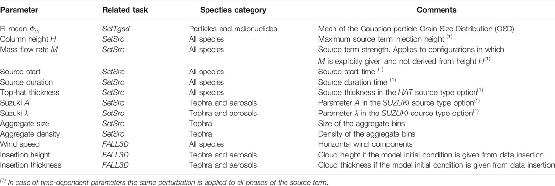
TABLE 1. List of model input parameters that can be perturbed in FALL3D-8.1 to generate ensemble runs. The related task and the species category affected are also indicated (see Folch et al. (2020), for details).

The ensemble generation starts with an unperturbed central member, which typically is set with the observed or “best-guess” input values and that, by construction, coincides with the “standard” single-run. For each parameter to be perturbed, the ensemble spread is then generated by sampling on the corresponding PDF around the unperturbed central value and within a range (amplitude) that spans the parameter uncertainty. For example, a perturbation of the source duration S_d by ± 1 h samples using either a linear or a Gaussian (centred at S_d) PDF within the interval [S_d − 1, S_d + 1]. For n ensemble members and m parameters (dimensions) perturbations result on a combination of n × m possible values that are then sub-sampled to define the n ensemble members using a classical Latin hypercube sampling algorithm (e.g., Husslage et al., 2006). This strategy guarantees that the spread across each of the m dimensions is maintained in the final member’s sub-sample. It is clear that the a priori generation of an ensemble requires expert judgement and involves some degree of subjectivity. The question on how an ensemble can be optimally generated is complex and falls beyond the scope of this manuscript. Nonetheless, a good practice if forecast observations exist is to check (a posteriori) that the ensemble-based forecast is statistically indistinguishable from observations by looking at the shape of the ensemble rank histogram.

2.2 Ensemble Postprocess Task

Once the model has run, the task PosEns merges all outputs from individual ensemble members in a single netCDF file containing ensemble-based deterministic and/or probabilistic outputs for all variables of interest (e.g., concentration at native model levels or at flight levels, cloud column mass, ground deposit load, etc). Options for ensemble-based deterministic outputs include the ensemble mean, the ensemble median, and values of user-defined percentiles. The standard deviation can be attached to any variable as a measure of the uncertainty of the deterministic outputs. On the other hand, ensemble-based probabilistic outputs can also be built by counting, at each grid point and time step, the fraction of ensemble members that verify a given condition, typically the exeedance of some threshold. For example, a probabilistic output for airborne volcanic ash can be defined based on the 2 mg/m³ concentration threshold in case of aviation-targeted products and counting, at each grid cell and time step, the fraction of members that overcome this value.

2.3 Model Validation Task

FALL3D-8.1 includes a third new task PosVal to validate both single-run (compatible with previous code versions) and ensemble-based deterministic and/or probabilistic outputs against various types of gridded and scattered observation datasets (see Table 2). Observation datasets include satellite-based observations and quantitative retrievals (to validate against cloud column mass), deposit isopach/isopleth maps, and point-wise deposit observations (to validate against deposit thickness or mass load). In all cases, this model task reads the required files, interpolates model and observations into the same grid and computes a series of categorical and quantitative validation metrics that are detailed in the following section. This model validation task inherits the model domain decomposition structure and, consequently, all metrics are first computed (in parallel) over each spatial sub-domain and then gathered and added to get global results over the whole computational domain.

TABLE 2

TABLE 2. Four types of observation datasets that can be used for model validation by task PosVal. The satellite detection and the satellite retrieval observation types stand, respectively, for detection (i.e. “yes/no” categorical observation) and quantitative column mass retrievals. The deposit contours observation type refers to isopach/isopleth deposit contours (e.g. from shape files or gridded maps). Finally, the deposit points stands for deposit thickness/load observations at scattered points. For each type of forecast, deterministic (D) or probabilistic (P), the Table indicates which validation metrics apply to each combination of observation-forecast types. The different generalised categorical and quantitative scores are defined in Section 3.

3 Ensemble Forecast Diagnostic Metrics

This section defines the different types of metrics computed by task PosVal, summarised in Table 3. These include: i) generalised categorical metrics, ii) quantitative metrics for deterministic forecasts and, iii) the ensemble rank histogram for ensemble-based probabilistic scenarios.

TABLE 3

TABLE 3. Summary of metrics. GMFS: Generalised Figure Merit of Space, GFAR: Generalised False Alarm Rate, GPPV: Generalised Positive Predictive Value, GPOD: Generalised Probability of Detection, GCCM: Generalised Composite Categorical Metric, BS: Brier Score, NRMSE: Normalised Root Mean Square Error.

3.1 Generalised Categorical Metrics

Categorical metrics (e.g., Jolliffe and Stephenson, 2012) apply to variables that take a limited number of values or “categories”. For example, in a deterministic forecast context it is common to define dichotomic categories (yes/no) for model and observations based on the occurrence (or not) of a given condition. At each observation point, this results on a 2 × 2 model-observations “contingency table” (true positives, true negatives, false positives, false negatives), from which a series of “geometric-based” or “contour-based” categorical metrics can be constructed, e.g., the probability of detection, the false alarm rate, etc. (Marti and Folch, 2018; Pardini et al., 2020). In this section, several classical categorical metrics widely used in deterministic forecast contexts are generalised to probabilistic forecasts with the objective of having a same set of forecast skill scores usable in both contexts.

Consider an ensemble-based model realisation with n ensemble members in a computational domain Ω. At each point and time instant, the forecasts of the n ensemble members can be ranked and the discrete probability of occurrence of a certain condition or threshold can be computed by simply counting how many ensemble members verify the condition (note that this results on n + 1 categories or probability bins). Let’s denote by P_m (x, t) the resulting discrete probability function defined in the domain Ω, where the subscript m stands for model and 0 ≤ P_m (x, t) ≤ 1. Clearly, P_m (x, t) = 0 implies that no ensemble member satisfies the condition at (x, t), whereas P_m(x, t) = 1 implies that all members do. In general, P_m (x, t) will be a function with finite support, that is, it will take non-zero values only over a sub-domain Ω_m(t) = {x ∈ Ω | P_m(x, t) > 0} where at least one ensemble member satisfies the condition. Let’s denote by δ_m(x, t) the step function defined from the support of P_m(x, t), that is:

${\delta }_m\left(x,t\right)=\left\{\begin{array}{cc}1\hfill & \text{if}x\in {\mathrm{\Omega }}_m\left(t\right)\hfill \\ 0\hfill & \text{if}x\notin {\mathrm{\Omega }}_m\left(t\right)\hfill \end{array}\right.(1)$

Note that the definitions of P_m(x, t) and δ_m(x, t) are also valid in a deterministic context. In fact, the deterministic forecast scenario represents the limit in which P_m(x, t) can take only two discrete values (0 or 1) and one simply has that Ω_m(t) = {x ∈ Ω | P_m(x, t) = 1} and P_m(x, t) = δ_m(x, t). From a geometrical point of view, δ_m(x, t) can be interpreted as the union of the n probability contours that define the discrete probability function P_m (x, t). In the deterministic limit, only one contour exists and, consequently, one has P_m(x, t) = δ_m(x, t).

Similar arguments can be followed regarding observations. In general, one could consider m different sources of observations and apply the same condition (threshold) to obtain a discrete probability function of observations P_o(x, t), define the subdomain Ω_o(t) = {x ∈ Ω | P_o(x, t) > 0} as the subset of Ω where at least one observation verifies the condition and, finally, define the resulting observations step function δ_ox, t) analogous to Eq. 1 but using Ω_o(t). Following with the analogy, this would result on a (n + 1) × (m + 1) model-observations “contingency table” for the most general case. In what follows, generalised categorical metrics will be defined for an arbitrary number of members/observations and grid projection. However, and for the sake of simplicity, only cases in which observations come from a single source (m = 1) will be considered here. As a result, it will be implicitly assumed that Ω_o(t) = {x ∈ Ω | P_o(x, t) = 1} and P_o(x, t) = δ_o (x, t). The following generalised categorical metrics are introduced:

3.1.1 Generalised Figure Merit of Space

The Generalised Figure Merit of Space (GFMS) is defined as:

$\text{GFMS}\left(t\right)=\frac{{\int }_{\mathrm{\Omega }}{\delta }_o{\delta }_m{P}_o{P}_{m}d\mathrm{\Omega }}{{\int }_{\mathrm{\Omega }}\left[\left(1-{\delta }_o\right)P_m+\left(1-{\delta }_m\right)P_o+{\delta }_o{\delta }_m{P}_o{P}_m\right]d\mathrm{\Omega }}(2)$

which, for the single-observation case considered here (P_o = δ_o) and using that ${\delta }_o^2={\delta }_o$, simplifies to:

$\text{GFMS}\left(t\right)=\frac{{\int }_{\mathrm{\Omega }}{\delta }_o{\delta }_m{P}_{m}d\mathrm{\Omega }}{{\int }_{\mathrm{\Omega }}\left[\left(1-{\delta }_o\right)P_m+\left(1-{\delta }_m\right){\delta }_o+{\delta }_o{\delta }_m{P}_m\right]d\mathrm{\Omega }}(3)$

Note that in the deterministic forecast limit (i.e., P_m = δ_m), the GFMS reduces to:

$\text{GFMS}\left(t\right)=\frac{{\int }_{\mathrm{\Omega }}{\delta }_o{\delta }_{m}d\mathrm{\Omega }}{{\int }_{\mathrm{\Omega }}\left[{\delta }_m+{\delta }_o-{\delta }_m{\delta }_o\right]d\mathrm{\Omega }}=\frac{{\mathrm{\Omega }}_o\cap {\mathrm{\Omega }}_m}{{\mathrm{\Omega }}_m+{\mathrm{\Omega }}_o-{\mathrm{\Omega }}_o\cap {\mathrm{\Omega }}_m}=\frac{{\mathrm{\Omega }}_o\cap {\mathrm{\Omega }}_m}{{\mathrm{\Omega }}_o\cup {\mathrm{\Omega }}_m}=\text{FMS}\left(t\right)(4)$

which is the classical definition of the Figure Merit of Space (FMS), also known as the Jaccard coefficient (e.g., Levandowsky and Winter 1971; Galmarini et al., 2010). From a geometric point of view, the FMS is interpreted as the ratio between the intersection of model-observations contours and its union. The GFMS introduced here has the same interpretation but using a weight-average with model/observations probability contours. The GFMS ranges from 0 (worst) to 1 (optimal). The continuous integrals over Ω in the expressions above are in practice computed by projecting observations into the model grid and summing the discrete probability bins over all grid cells. For example, in the case of Eq. 3, the discrete computation would be as:

$\text{GFMS}\left(t\right)=\frac{{\sum }_j{H}_j{\delta }_{oj}{\delta }_{mj}{P}_{mj}}{{\sum }_j{H}_j\left(1-{\delta }_{oj}\right)P_{mj}+{\sum }_j{H}_j\left(1-{\delta }_{mj}\right){\delta }_{oj}+{\sum }_j{H}_j{\delta }_{oj}{\delta }_{mj}{P}_{mj}}(5)$

where H_j = m_1jm_2jm_3jV_j is the grid mapping factor of the j grid cell, V_j is the cell volume, and m_xj are the mapping factors depending on the coordinate system (see Tables 8 and 9 in Folch et al., 2020). Note that in the deterministic limit and for the particular case of a regular Cartesian grid (i.e., all cells equal, unit map factors) this further simplifies to:

$\text{FMS}\left(t\right)=\frac{{\sum }_j{\delta }_{oj}{\delta }_{mj}}{{\sum }_j\left(1-{\delta }_{oj}\right){\delta }_{mj}+{\sum }_j\left(1-{\delta }_{mj}\right){\delta }_{oj}+{\sum }_j{\delta }_{oj}{\delta }_{mj}}=\frac{\text{TP}}{\text{FP\hspace{0.17em}}+\text{\hspace{0.17em}FN\hspace{0.17em}}+\text{\hspace{0.17em}TP}}(6)$

and coincides with the number of True Positives (TP) divided by the number of False Positives (PF) + False Negatives (FN) + True Positives (TP), which is also the classical non-geometric interpretation of the FMS (e.g., Pardini et al., 2020). However, in general, the computation of the GFMS in non-regular coordinate systems (5) takes into account a cell-dependent weight proportional to the cell volume (area) through the grid mapping factors H_j.

3.1.2 Generalised False Alarm Rate

The Generalised False Alarm Rate (GFAR) is defined as:

$\text{GFAR}\left(t\right)=\frac{{\int }_{\mathrm{\Omega }}\left(1-{\delta }_o\right){\delta }_m{P}_{m}d\mathrm{\Omega }}{{\int }_{\mathrm{\Omega }}\left[\left(1-{\delta }_o\right){\delta }_m{P}_m+{\delta }_o{\delta }_m{P}_o{P}_m\right]d\mathrm{\Omega }}(7)$

which, for the case of single set of observations (P_o = δ_o), reduces to:

$\text{GFAR}\left(t\right)=\frac{{\int }_{\mathrm{\Omega }}\left(1-{\delta }_o\right){\delta }_m{P}_{m}d\mathrm{\Omega }}{{\int }_{\mathrm{\Omega }}\left[\left(1-{\delta }_o\right){\delta }_m{P}_m+{\delta }_o{\delta }_m{P}_m\right]d\mathrm{\Omega }}(8)$

In the deterministic forecast limit (P_m = δ_m), the definition of the GFAR further simplifies to:

$\text{GFAR}\left(t\right)=\frac{{\int }_{\mathrm{\Omega }}\left(1-{\delta }_o\right){\delta }_{m}d\mathrm{\Omega }}{{\int }_{\mathrm{\Omega }}{\delta }_{m}d\mathrm{\Omega }}=\frac{{\mathrm{\Omega }}_m-{\mathrm{\Omega }}_o\cap {\mathrm{\Omega }}_m}{{\mathrm{\Omega }}_m}=1-\frac{{\mathrm{\Omega }}_o\cap {\mathrm{\Omega }}_m}{{\mathrm{\Omega }}_m}=\text{FAR}\left(t\right)(9)$

which is the classical definition of the False Alarm Rate (FAR) (e.g., Kioutsioukis et al., 2016). In the geometric interpretation, the GFAR can be viewed as the fraction of Ω_m with false positives but generalised to probabilistic contours, and it ranges from 0 (optimal) to 1 (worst). Again, the continuous integrals in Eq. 8 are computed in practice over the model grid as:

$\text{GFAR}\left(t\right)=\frac{{\sum }_j{H}_j\left(1-{\delta }_{oj}\right){\delta }_{mj}{P}_{mj}}{{\sum }_j{H}_j\left(1-{\delta }_{oj}\right){\delta }_{mj}{P}_{mj}+{\sum }_j{H}_j{\delta }_{oj}{\delta }_{mj}{P}_{mj}}(10)$

which, in the deterministic limit and for a regular grid (H_j = 1), further simplifies to:

$\text{FAR}\left(t\right)=\frac{{\sum }_j\left(1-{\delta }_{oj}\right){\delta }_{mj}}{{\sum }_j\left(1-{\delta }_{oj}\right){\delta }_{mj}+{\sum }_j{\delta }_{oj}{\delta }_{mj}}=\frac{\text{FP}}{\text{FP\hspace{0.17em}}+\text{\hspace{0.17em}TP}}(11)$

and therefore coincides, in a non-geometric interpretation, with the number of False Positives (FP) divided by the number of False Positives (FP) + True Positives (TP).

3.1.3 Generalised Positive Predictive Value

The Generalised Positive Predictive Value (GPPV) is defined as the complement of the GFAR:

$\text{GPPV}\left(t\right)=1-\text{GFAR}\left(t\right)=\frac{{\int }_{\mathrm{\Omega }}{\delta }_o{\delta }_m{P}_o{P}_{m}d\mathrm{\Omega }}{{\int }_{\mathrm{\Omega }}\left[\left(1-{\delta }_o\right){\delta }_m{P}_m+{\delta }_o{\delta }_m{P}_o{P}_m\right]d\mathrm{\Omega }}(12)$

Analogously, for the single-observation case (P_o = δ_o):

$\text{GPPV}\left(t\right)=\frac{{\int }_{\mathrm{\Omega }}{\delta }_o{\delta }_m{P}_{m}d\mathrm{\Omega }}{{\int }_{\mathrm{\Omega }}\left[\left(1-{\delta }_o\right){\delta }_m{P}_m+{\delta }_o{\delta }_m{P}_m\right]d\mathrm{\Omega }}(13)$

or

$\text{GPPV}\left(t\right)=\frac{{\sum }_j{H}_j{\delta }_{oj}{\delta }_{mj}{P}_{mj}}{{\sum }_j{H}_j\left(1-{\delta }_{oj}\right){\delta }_{mj}{P}_{mj}+{\sum }_j{H}_j{\delta }_{oj}{\delta }_{mj}{P}_{mj}}(14)$

In the deterministic limit Eq. 13 yields to the classical Positive Predictive Value (PPV), also known as the model precision (Pardini et al., 2020):

$\text{GPPV}\left(t\right)=\frac{{\int }_{\mathrm{\Omega }}{\delta }_o{\delta }_{m}d\mathrm{\Omega }}{{\int }_{\mathrm{\Omega }}{\delta }_{m}d\mathrm{\Omega }}=\frac{{\mathrm{\Omega }}_o\cap {\mathrm{\Omega }}_m}{{\mathrm{\Omega }}_m}=\text{PPV}\left(t\right)(15)$

The GPPV ranges from 0 (worst) to 1 (optimal) and geometrically can be interpreted as the fraction of Ω_m with true positives (model hits) but for probabilistic contours. Again, in a regular Cartesian grid the discrete version of Eq. 15 coincides with the number of True Positives (TP) divided by the number of False Positives (FP) + True Positives (TP):

$\text{PPV}\left(t\right)=\frac{{\sum }_j{\delta }_{oj}{\delta }_{mj}}{{\sum }_j\left(1-{\delta }_{oj}\right){\delta }_{mj}+{\sum }_j{\delta }_{oj}{\delta }_{mj}}=\frac{\text{TP}}{\text{FP\hspace{0.17em}}+\text{\hspace{0.17em}TP}}(16)$

3.1.4 Generalised Probability of Detection

The Generalised Probability of Detection (GPOD) is defined as:

$\text{GPOD}\left(t\right)=\frac{{\int }_{\mathrm{\Omega }}{\delta }_o{\delta }_m{P}_o{P}_{m}d\mathrm{\Omega }}{{\int }_{\mathrm{\Omega }}\left[\left(1-{\delta }_m\right){\delta }_o{P}_o+{\delta }_o{\delta }_m{P}_o{P}_m\right]d\mathrm{\Omega }}(17)$

which, for the single-observation case (P_o = δ_o), reduces to:

$\text{GPOD}\left(t\right)=\frac{{\int }_{\mathrm{\Omega }}{\delta }_o{\delta }_m{P}_{m}d\mathrm{\Omega }}{{\int }_{\mathrm{\Omega }}\left[\left(1-{\delta }_m\right){\delta }_o+{\delta }_o{\delta }_m{P}_m\right]d\mathrm{\Omega }}(18)$

As with the other metrics, in the deterministic limit (P_m = δ_m) the GPOD simplifies to:

$\text{GPOD}\left(t\right)=\frac{{\int }_{\mathrm{\Omega }}{\delta }_o{\delta }_{m}d\mathrm{\Omega }}{{\int }_{\mathrm{\Omega }}{\delta }_{o}d\mathrm{\Omega }}=\frac{{\mathrm{\Omega }}_o\cap {\mathrm{\Omega }}_m}{{\mathrm{\Omega }}_o}=\text{POD}\left(t\right)(19)$

and coincides with the Probability of Detection (POD), also known as the model sensitivity (Pardini et al., 2020). The GPOD ranges from 0 (worst) to 1 (optimal) and, geometrically, is interpreted as the fraction of Ω_o with true positives. Again, in the discrete space (18) yields to:

$\text{GPOD}\left(t\right)=\frac{{\sum }_j{H}_j{\delta }_{oj}{\delta }_{mj}{P}_{mj}}{{\sum }_j{H}_j\left(1-{\delta }_{mj}\right){\delta }_{oj}+{\sum }_j{H}_j{\delta }_{oj}{\delta }_{mj}{P}_{mj}}(20)$

that in a regular grid and deterministic limit coincides with the number of True Positives (TP) divided by the number of False Negatives (FN) + True Positives (TP):

$\text{POD}\left(t\right)=\frac{{\sum }_j{\delta }_{oj}{\delta }_{mj}}{{\sum }_j\left(1-{\delta }_{mj}\right){\delta }_{oj}+{\sum }_j{\delta }_{oj}{\delta }_{mj}}=\frac{\text{TP}}{\text{FN\hspace{0.17em}}+\text{\hspace{0.17em}TP}}(21)$

3.1.5 Generalised Composite Categorical Metric

It can be anticipated that some generalised categorical metrics can vary oppositely when comparing single-run and ensemble-based simulations. For example, one may expect that a large ensemble spread yields to a larger GPOD but, simultaneously, also to larger GFAR. In order to see how different metrics counterbalance we introduce the Generalised Composite Categorical Metric (GCCM) as:

$\text{GCCM}=\frac{\text{GFMS\hspace{0.17em}}+\text{\hspace{0.17em}GPPV\hspace{0.17em}}+\text{\hspace{0.17em}GPOD}}{3}=\frac{\text{GFMS}+\left(1-\text{GFAR}\right)+\text{\hspace{0.17em}GPOD}}{3}(22)$

where the factor 3 is introduced to normalise GCCM in the range 0 (worst) to 1 (optimal). This multi-composite definition is analogous to what is done for the SAL, defined as the sum of Structure, Amplitude and Location (e.g., Marti and Folch, 2018).

3.1.6 Brier Score

The Brier Score (BS) is defined as:

$\text{BS}=\frac{{\int }_{{\mathrm{\Omega }}_o}{\left(P_m-P_o\right)}^{2}d\mathrm{\Omega }}{{\int }_{{\mathrm{\Omega }}_o}d\mathrm{\Omega }}(23)$

which, for the single-observation case, reduces to:

$\text{BS}=\frac{{\int }_{{\mathrm{\Omega }}_o}{\left(P_m-{\delta }_o\right)}^{2}d\mathrm{\Omega }}{{\int }_{{\mathrm{\Omega }}_o}d\mathrm{\Omega }}(24)$

Note that the above integrals are constrained to the subdomain Ω_o where observations exist. The Brier score is the averaged squared error of a probabilistic forecast and ranges from 0 (optimal) to 1 (worst). In the discrete space, Eq. 24 is computed as:

$\text{BS}=\frac{{\sum }_j{H}_j{\delta }_{oj}{\left(P_{mj}-1\right)}^2}{{\sum }_j{H}_j{\delta }_{oj}}(25)$

which, in a regular Cartesian grid, reduces to the more standard definition of the Brier score (Brier, 1950):

$\text{BS}=\frac{1}{n_o}\sum _{j=1}^{n_o}{\left(P_{mj}-1\right)}^2(26)$

where n_o is the total number of observation points.

3.2 Quantitative Scores

As a quantitative metric for deterministic forecasts we consider the Normalised Root Mean Square Error (NRMSE), defined as:

$\text{NRMSE}=\frac{\sqrt{\frac{1}{n_o}\sum {\left(M_i-O_i\right)}^2}}{O_{max}-O_{\mathit{min}}}(27)$

where O_i are the n_o observation values, M_i is the model value at the ith observation point, and O_max and O_min are, respectively, the maximum and minimum of the observations (at the considered time step). Note that, as opposed to the previous categorical metrics, this quantitative score is valid only for deterministic forecasts (single-run or ensemble-based).

3.3 Ensemble Rank Metrics

The observations rank histogram or Talagrand diagram (Talagrand et al., 1997) is commonly used a posteriori to measure the consistency of an ensemble forecast and to assess whether observations are statistically indistinguishable from the ensemble members. The histogram can be used to recalibrate ensemble forecasts and it is constructed as follows. For each observation (grid point and time), the n ensemble members are ranked from lowest to highest using the variable of interest (column mass, deposit thickness, etc.) and the rank of the observation with respect to the forecast is identified and added to the corresponding bin (points with zero observation values are not counted). Flat histograms indicate a consistent forecast, with an observed probability distribution well represented by the ensemble. Asymmetric histograms indicate positive/negative forecast bias, as most observations often rank below/above the extremes respectively. Finally, dome-shaped/U-shaped histograms indicate over/under forecast dispersion and reflect too large/small ensemble spread respectively. Other common metrics to evaluate ensembles, e.g., the spread-skill relationship (e.g., Scherrer et al., 2004), are not considered at this stage but will be incorporated in future code versions.

4 Application Cases

4.1 The July 2018 Ambae SO₂ Cloud

In April and July 2018 the Ambae volcano (Vanuatu archipelago) produced two paroxysm eruptions that injected large amounts of SO₂ reaching the tropopause (Moussallam et al., 2019). According to Himawari-8 satellite observations, the July 26, 2018 phase started before 12 UTC (23:00 LT) and lasted for about 4 h. Kloss et al. (2020) estimated an atmospheric SO₂ injection height of either 18 or 14 km a.s.l. by co-locating ERA5 temperature profiles and Brightness Temperature observations. To generate our SO₂ validation dataset we apply the 3-band interpolation procedure proposed by Prata et al. (2004) to measurements made by the Advanced Himawari Imager (AHI) aboard Himawari-8. Details of the method can be found in Appendix B of Prata et al. (2021). To estimate the total mass we only considered pixels containing more than 20 DU within a spatial domain from 160–200°E to 5–25°S. We also applied a Gaussian filter to generate smoothed contours around the SO₂ clouds to filter out pixels greater than 20 DU that were far from source (i.e., false detections). Our results show that, during our satellite analysis period (from 26 July at 09:00 UTC to 31 July at 09:00 UTC), maximum total mass of 323005E;86_90 kt was injected into the upper atmosphere, where 86 and 90 kt are asymmetric errors around the best estimate (323 kt). The first significant injection of SO₂ occurred at around 10:00 UTC on 26 July and reached its maximum (253 kt) at 23:00 UTC. A second eruption occurred at around on 27 July at 01:00 UTC, and added a further 70 kt of SO₂. These SO₂ mass estimates are in broad agreement with independent TROPOMI SO₂ standard product mass retrievals (360 ± 40 kt), that assume a 15 km high SO₂ layer with 1 km thickness (Malinina et al., 2020).

Based on the observations available during or shortly after the eruption, a single-run FALL3D-8.1 simulation was configured considering one SO₂ (aerosol) bin and an emission starting on 26 July at 10:00 UTC (21:00 LT) lasting for 4 h, assuming a top-hat plume vertical profile with the top at 16 km a.s.l. and a total emitted mass of 290 kt (emission rate 2 × 104 kg/s). This reference run represents a typical operational procedure during or shortly after an eruption, when model inputs are set with the uncertain available information. From this “best-guess” central member, an ensemble with 64 members was defined by perturbing the eruption start time (perturbation range of ±1 h), the eruption duration (±1 h), the cloud injection height H (±2 km), the thickness T of the top-hat emission profile (±2 km), the eruption rate (±30%), and the driving ERA-5 wind field as shown in Table 4. For both single-run and ensemble-based forecasts, the model grid resolution is 0.05^o in the horizontal and 250 m in the vertical, with the top of the computational domain placed at 22 km a.s.l.

TABLE 4

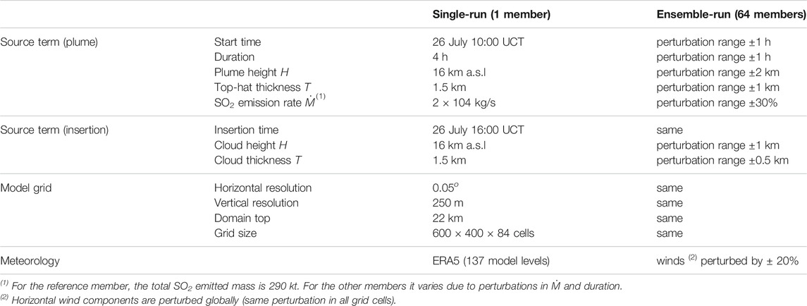
TABLE 4. Model setup for the July 26, 2018 single-run and ensemble-based (64 members) Ambae SO₂ simulations.

Model runs generate hourly outputs concurrent with the AHI cloud mass retrievals over the forecast period. Figure 1 compares AHI SO₂ column mass retrievals with different deterministic forecast outputs, namely the single-run, the ensemble mean, and the ensemble median at one particular instant (July 28, 2018 at 00:00 UTC). The ensemble mean and median produce a more diffused cloud, partly due to wind shear effects. Time series of quantitative scores, e.g., using the NRMSE (Eq. 27), are automatically generated by the FALL3D-8.1 model task PosVal. Figure 2 shows time series of NRMSE for different deterministic forecast options (single run, ensemble mean, and ensemble median). As observed, this metric follows a similar trend in all cases but the gain from the ensemble-based approaches is very clear: the deterministic ensemble-based options reduce the forecast NRMSE by a factor between two and three in most time instants. For comparative purposes, Figure 2 also shows what happens if the data insertion mechanism is used to initialise the model runs instead of the source option. Data insertion consists of initialising a model run with an effective virtual source inserted away from the source, and FALL3D admits this initialisation option from column load satellite retrievals (Prata et al., 2021). This represents a case with better constrained input data (initial conditions) and, as expected, the data insertion option yields lower values of the NRMSE and shows little differences among the single-run and ensemble-based approaches.

FIGURE 1

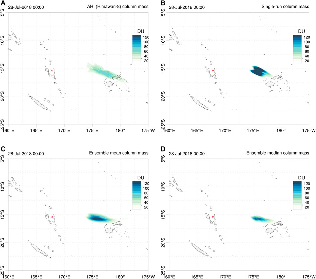
FIGURE 1. Comparison between: (A) Ambae AHI SO₂ column mass retrievals, (B) single-run (unperturbed central member), (C) ensemble mean deterministic forecast, (D) ensemble median deterministic forecast. All snapshots correspond to July 28, 2018 at 00:00 UTC. Contours in Dobson Units (DU). Red circle shows the location of Ambae volcano.

FIGURE 2

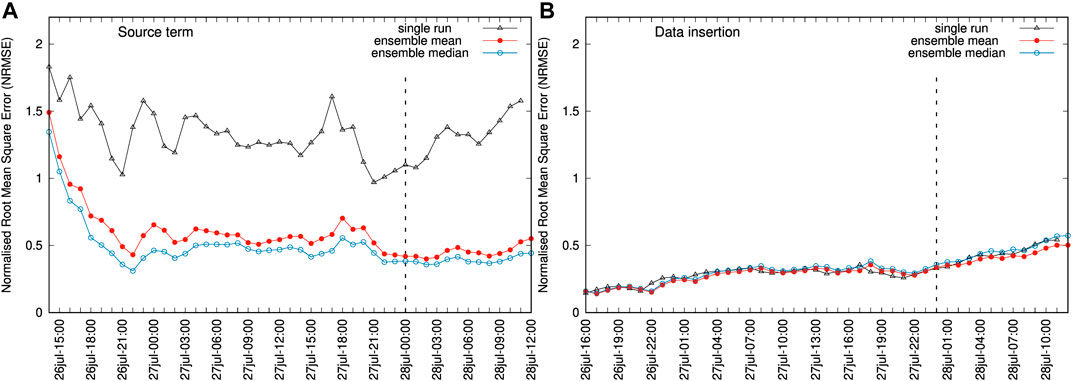
FIGURE 2. (A) Time series of Normalised Root Mean Square Error (NRMSE) for the Ambae single-run (black line), ensemble mean (red line), and ensemble median (blue line). The vertical dashed line marks the instant of the snapshot shown in Figure 1. Symbols indicate the hourly AHI retrievals. (B) Same but with the source term given by a data insertion mechanism. In this case, the ensemble is defined by perturbing only the height and thickness of the injected cloud as indicated in Table 4. Plots on the same vertical scale.

As discussed in Section 2.2, probabilistic outputs can be generated from a given condition by counting the fraction of ensemble members that exceed a threshold value. For example, Figure 3 shows 20 Dobson Units (DU) contours of SO₂ column mass for deterministic and probabilistic forecasts, where the value of 20 is assumed as representative of the SO₂ detection threshold in the AHI retrievals. These contours can be used for forecast validation using generalized categorical metrics that allow, on one side, to quantify the gain in the ensemble-based cases with respect to the reference single-run and, on the other side, to compare objectively the different ensemble-based approaches. To these purposes, Figure 4 plots the time series of different generalised categorical metrics, GFMS (Eq. 5), GPOD (Eq. 20), and GCCM (Eq. 22) together with the BS (Eq. 25), the latter for the probabilistic case only. As expected, the ensemble mean outperforms the reference run in all the metrics, with substantial gain in GFMS and GPOD, yielding to better generalised composite metric GCCM. This is not true for the ensemble median, which presents similar forecast skills than those of the single run. On the other hand, the probabilistic approach behaves similarly to the ensemble mean in terms of GCCM because the larger false alarm rate is counterbalanced by a higher probability of detection. No conclusion can be extracted from this example on whether the probabilistic forecast option outperforms the deterministic ensemble mean or not. Finally, the observations rank histogram over the considered period (see Figure 5A) shows an acceptably flat histogram (reflecting good ensemble spread) although with a slight bias towards members having larger SO₂ mass. This skewing can be due to errors in cloud location, errors in amplitude, or to a combination of both. However, an inspection to the time series of AHI total retrieved mass (Figure 5B) suggests that the ensemble spread in cloud mass is adequate, indicating co-location as the reason for skewing. In fact, we performed successive ensemble redefinition runs (increasing mass in the reference run) and observed that the ensemble histogram flattened but, at the same time, this did not imply better values of the generalized metrics.

FIGURE 3

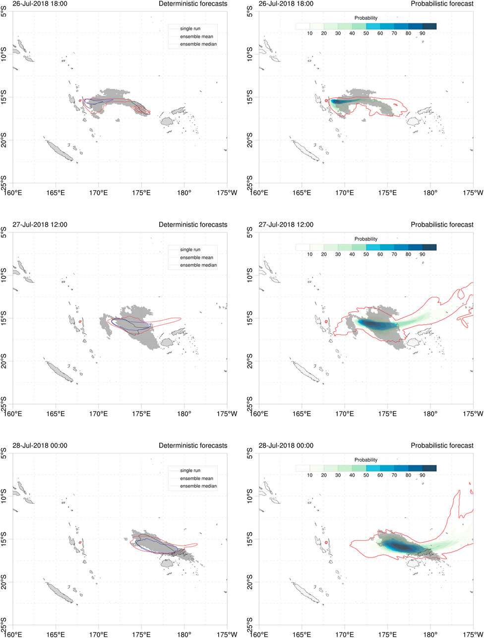
FIGURE 3. Contours of 20 DU SO₂ column mass for deterministic (left) and probabilistic (right) Ambae forecasts at three different instants; 26 July at 18:00UTC (top), 27 July at 12:00 UTC (middle) and 28 July at 00:00UTC (bottom). In the probabilistic approach, contours give the probability (in %) to exceed 20 DU. The outer red contour indicates the 1.56% (1/64) probability. The grey shaded area shows the corresponding 20 DU from AHI retrievals. Red circle shows the location of Ambae volcano.

FIGURE 4

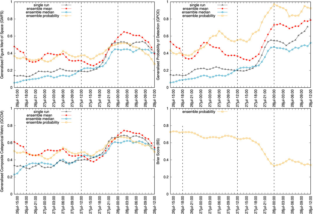
FIGURE 4. Time series of generalised categorical metrics for deterministic (single run and ensemble-based) and probabilistic Ambae forecasts using the 20 DU SO₂ column mass contours. Plots show GFMS (top left), GPOD (top right), GCCM (bottom left) and BS (bottom right). Symbols indicate the instants of the AHI retrievals. The three vertical dashed lines mark the instants of the snapshots shown in Figure 3. Note that for the BS only the probabilistic option applies.

FIGURE 5

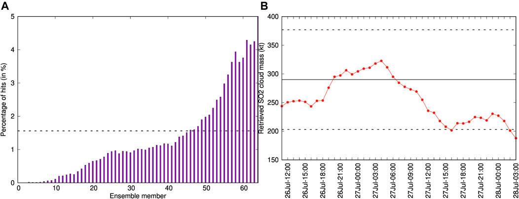
FIGURE 5. (A) Observations rank histogram (Talagrand diagram) for the 64-member Ambae ensemble run. The horizontal dashed line at 1/64 = 1.56% indicates a perfectly consistent forecast, with all its members being equally represented against observations. (B) time series of SO₂ AHI retrieved cloud mass. The solid horizontal line at 290 kt shows the reference run and the dashed lines indicate the ±30% ensemble spread in emission rate.

4.2 The April 2015 Calbuco Ash Cloud and Deposit

The Calbuco volcano (Chile) reawakened in 2015 with two major eruptive pulses on 22 April at 21:08 UTC and 23 April at about 04:00 UTC respectively, followed by a third minor event on the following day (e.g., Reckziegel et al., 2016). According to C-band dual-polarisation radar observations, the maximum ash plume heights exceeded 20 km above sea level in the surrounding area of the Calbuco volcano (Vidal et al., 2017). Subsequent plume modelling and field studies on the tephra fallout deposits indicated that the sub-Plinian phases, with similar column heights exceeding 15 km a.s.l. blanked the region with a total erupted volume ranging between 0.28 and 0.58 km³ and a deposit mass in the range 2–7 × 1011 kg depending on different estimations (Romero et al., 2016; Van Eaton et al., 2016). On the other hand, ash cloud mass estimations from Moderate Resolution Imaging Spectroradiometer (MODIS) and Visible Infrared Imaging Radiometer Suite (VIIRS) indicated 1–3 × 109 kg of distal airborne material (e.g., Marzano et al., 2018), suggesting $<1\%$ of remaining fine ash in the distal cloud. The comparison with field-based reconstructed particle grain size distributions, entailing a much larger fraction of mass in the fine tail (Reckziegel et al., 2016), point at the occurrence of substantial fine ash aggregation, as corroborated also by in-situ deposit observations. The Calbuco eruptions also entailed substantial co-located emissions of SO₂ at 15 km a. v.l. in the range of 300 kt for the two phases according to GOME-2 satellite images (Pardini et al., 2017).

To show how ensemble ash simulations can be validated at high temporal resolution with qualitative ash cloud observations, we use satellite data collected from the SEVIRI instrument aboard Meteosat-10. Following the ash detection method presented in Appendix A of Prata et al. (2021), we generated binary (ash/no ash) fields at 1 h time-steps from 22 April at 23:00 UTC to 26 April at 23:00 UTC within a domain from 0–75°W to 15–55°S. We did not consider quantitative retrievals for this eruption as Calbuco is located outside of the SEVIRI field of view, which meant that many of the pixels detected as ash at the beginning of the eruption were associated with high satellite zenith angles ($>\mathrm{75}°$) where retrievals can be unreliable. On the other hand, thickness measurements of fallout deposits from the 22–23 April 2015 eruption of Calbuco volcano were reported at 163 sites by Van Eaton et al. (2016) within a radius of 500 km. Romero et al. (2016) used thickness measurements to reconstruct the fallout deposit distribution by hand-drawing the corresponding isopach maps. A remarkable feature of the distal deposit is the presence of a secondary thickness maximum in the region around Junín de los Andes and Piedra del Aguila (Argentina, around 300 km downwind), indicating the occurrence of a complex plume dynamics involved during the eruption. Here, two independent deposit datasets are used to validate the Calbuco simulations: i) the deposit contours (isopachs) generated by Romero et al. (2016) for 0.1, 0.5, 1 and 2 mm (Van Eaton, personal communication) and, ii) the deposit point thickness at 159 sites reported by Van Eaton et al. (2016). Note that ambiguous data from 4 sites were removed from the original dataset.

For the Calbuco case, the ensemble reference run was configured with 20 tephra bins ranging in size from Φ = − 2 (4 mm) to Φ = 7 (8 μm) and including one bin of aggregates. The plume source term consists of 2 phases lasting 1.5 and 6 h respectively, with a Suzuki vertical profile (A = 5, λ = 3) reaching 16 km a.s.l. and a total emitted mass of 6 × 10¹¹ kg. The 64-member ensemble was built by perturbing the most relevant source, granulometry and wind parameters as shown in Table 5. As for the previous Ambae case, the model grid resolution is 0.05^o in the horizontal and 250 m in the vertical, with the top of the computational domain placed at 20 km a.s.l. An ensemble with 64 members was defined by perturbing the starting time of the phases (±1 h), its duration (±1 h), the plume height H (±2 km), the dimensionless Suzuki parameters A (±3) and λ (±2), the mean of the particle size distribution Φ_m (±1), and the size (±100 μm) and density (±100 kg/m³) of the aggregates.

TABLE 5

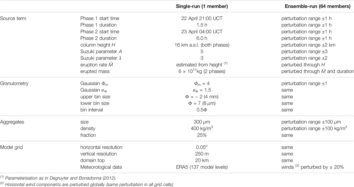
TABLE 5. Model setup for the April 22, 2015 single-run and ensemble-based (64 members) Calbuco tephra simulations.

Figure 6 compares single-run and ensemble-based deterministic runs at 159 deposit observation points that span almost 4 orders of magnitude in tephra thickness. On a point-by-point basis, the ensemble mean run reduces the differences with observations in 107 out of 159 points (67%), whereas the single-run reference still gives a closer fit in 52 points (33%). In contrast, the ensemble median can only improve on 64 points (40%), outperforming the reference run values only in the proximal (Figure 6B). In terms of overall NRMSE, the ensemble mean gives 0.11 as opposed to a 0.13 for the other two deterministic options, i.e. a 16% of overall improvement (Table 6).

FIGURE 6

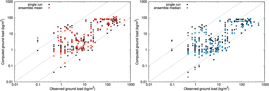
FIGURE 6. Validation of Calbuco runs in 159 deposit points. Deposit thicknesses are converted to deposit loads (kg/m²) assuming an averaged density of 1,000 kg/m³. Left: single-run (black points) versus ensemble mean (red points). Right: single-run (black points) versus ensemble median (blue points). For reference, the three dashed lines show the perfect fit and the 10 model over and under-estimation bounds. The resulting global values of the NRMSE are reported in Table 6.

TABLE 6

TABLE 6. Validation of the April 22, 2015 Calbuco simulations with deposit thickness at scattered deposit points. Percentage means the fraction of points that reduce differences with observations with respect to the reference single-run. Best values highlighted in green.

In addition to the deposit points, the deposit isopach contours provide a second dataset for deposit validation based on generalised categorical metrics (see Table 2). Figure 7 shows the different deterministic forecast contours compared with the 0.1, 0.5, 1, and 2 mm isopachs reported by Romero et al. (2016), characteristic of intermediate (few hundreds of km) to more proximal (up to around 100 km) distances to source. On the other hand, Figure 8 shows the probabilistic counterpart, with the ensemble probability contours giving the probability to exceed each corresponding isopach value. The resulting values for generalised metrics and Brier score are reported in Table 7, which includes also an additional more proximal contour of 4 mm (not shown in the previous Figures). For deterministic approaches, the ensemble mean clearly outperforms the reference run and the ensemble median (with the only exception of GFAR) across all distances. However, best overall results are obtained by probabilistic forecasts, particularly for GFMS and GPOD. In terms of the composite metric (GCCM), the ensemble mean is slightly better in the distal and the probabilistic in the proximal but, again, it is not clear which of these two options performs better.

FIGURE 7

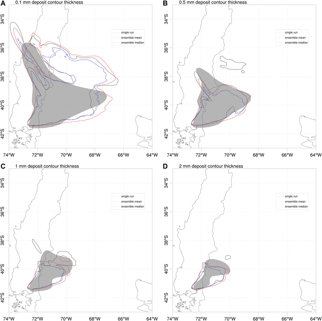
FIGURE 7. Validation of Calbuco deterministic forecasts using deposit isopach contours of 0.1, 0.5, 1, and 2 mm. Model results for single-run (black line), ensemble mean (red line) and ensemble median (blue line). Grey-filled areas show the corresponding isopachs estimated by Romero et al. (2016) from extrapolation of deposit point measurements. Red circle shows the location of Calbuco volcano. The resulting values of generalised categorical metrics are reported in Table 7.

FIGURE 8

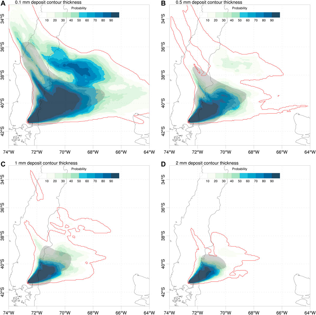
FIGURE 8. Validation of Calbuco probabilistic forecasts with deposit isopach contours. Color contours give the model probability (in %) for deposit thickness to exceed 0.1, 0.5, 1, and 2 mm. Grey-filled areas show the corresponding isopachs estimated by Romero et al. (2016) from extrapolation of deposit point measurements. The outer red contour indicates the 1.56% (1/64) probability. Red circle shows the location of Calbuco volcano. The resulting values of generalised categorical metrics and Brier Score (BS) are reported in Table 7.

TABLE 7

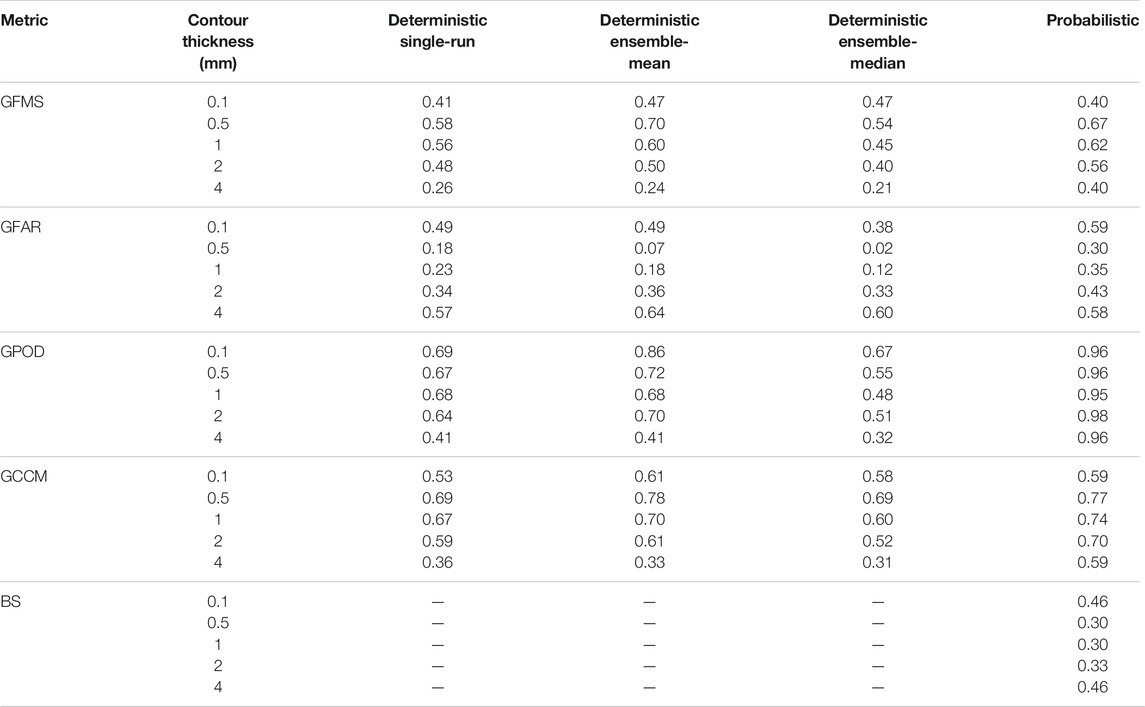
TABLE 7. Validation of the April 22, 2015 Calbuco simulations with deposit isopach contours from Romero et al (2016). Five deposit isopach values of 0.1, 0.5, 1, 2, and 4 mm are considered. Best values for each metric and contour are highlighted in green. The Brier Score (BS) applies only to the probabilistic approach.

Finally, the Calbuco ash cloud can also be validated with satellite imagery. Given the limitations of the dataset (as explained above) we do not consider ash retrievals as reliable and use the SEVIRI ash detection option instead. Figures 9, 10 show, respectively, snapshots of deterministic and probabilistic cloud mass contours (0.1 g/m² is assumed as a detection threshold) and time series of generalised categorical metrics. Model to observations miss-matches are more evident than for the Ambae case, partly due to the aforementioned reasons. However, similar conclusions can be extracted about the improvements in the ensemble mean and probabilistic cases. Again, the ensemble median (blue curves) worsens the single-run forecast skills.

FIGURE 9

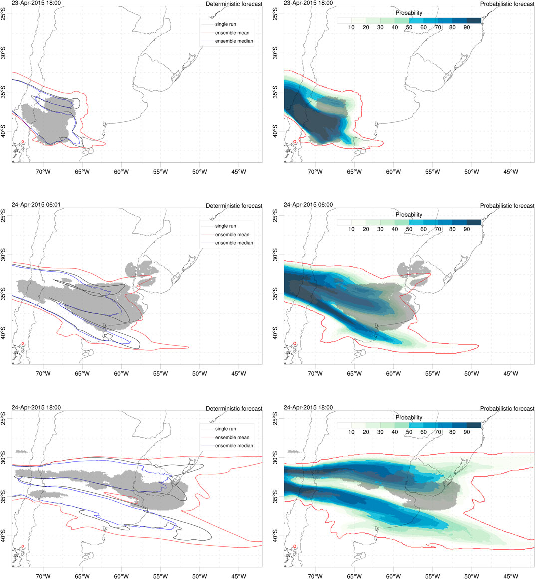
FIGURE 9. Validation of Calbuco ash cloud with the satellite detection (SEVIRI ash flag) observation dataset. Model column mass contours of 0.1 g/m² for deterministic (left) and probabilistic (right) forecasts at three different instants; 23 April at 18:00UTC (top), 24 April at 06:00 UTC (middle) and 24 April at 18:00UTC (bottom). In the probabilistic plots, the outer red contour indicates the 1.56% (1/64) probability. The shaded areas show the contours encompassing SEVIRI ash flagged pixels. Red circle shows the location of Calbuco volcano.

FIGURE 10

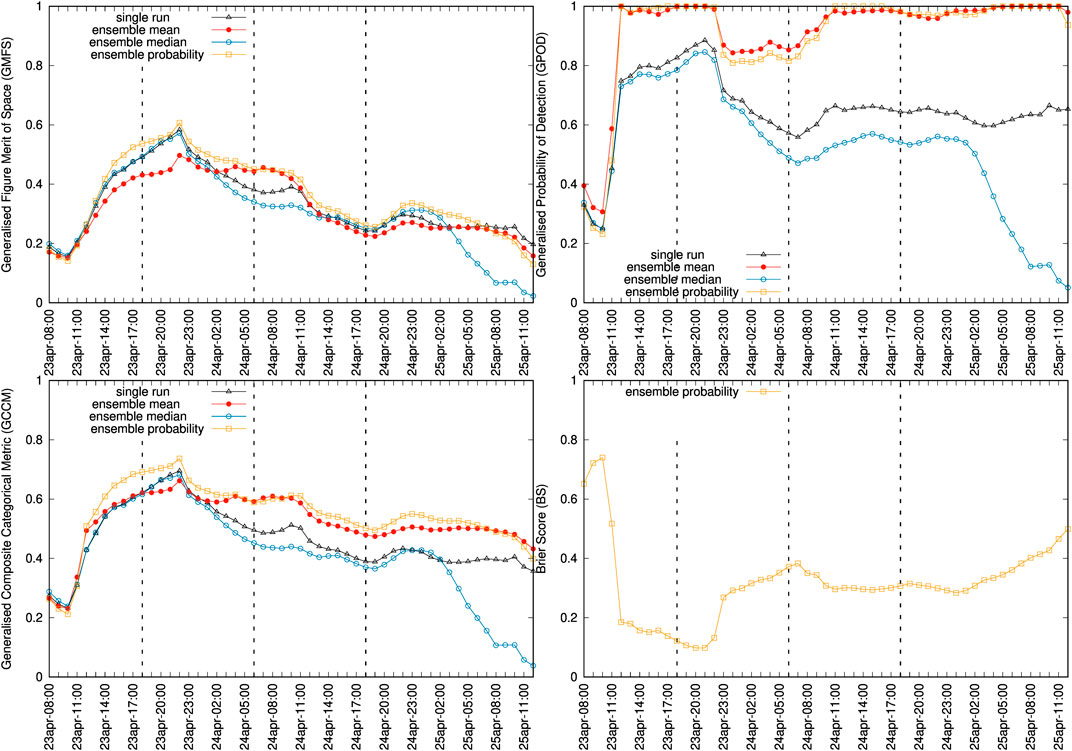
FIGURE 10. Time series of generalised categorical metrics for deterministic (single run and ensemble-based) and probabilistic forecasts using the 0.1 g/m² ash column mass contours. Plots show GFMS (top left), GPOD (top right), GCCM (bottom left) and BS (bottom right). Symbols indicate the instants of SEVIRI retrievals. The vertical dashed lines mark the three instants plot in Figure 9. Note that for the BS only the probabilistic option applies.

5 Summary and Discussion

The last version release (v8.1) of FALL3D allows configuring, running, post-processing and eventually validating ensemble-based forecasts in a single embarrassingly parallel workflow. The ensemble runs, built from perturbing the most uncertain input parameters of a reference ensemble member, can furnish an array of deterministic forecasts with an associated uncertainty and/or probabilistic products based on the occurrence (or not) of certain exeedance or threshold conditions. Different types of metrics can be considered in FALL3D-8.1 for model validation (see Table 2), including novel categorical metrics resulting from the generalisation to probabilistic scenarios of classic geometric-based indicators (FMS, POD, FAR, etc). The skills of the ensemble-based modelling approaches have been compared against single-runs (and among them) using different types of observations. On one hand, satellite retrievals of cloud mass have been considered for validation of the July 2018 Ambae SO₂ clouds (Table 4). On the other, tephra deposit thickness observations at 159 locations and resulting deposit isopach contours have been used, together with satellite ash cloud detection, i.e. yes/no ash flagged pixels, for the April 2015 Calbuco eruption (Table 5). An ensemble of 64 members with a model spatial resolution of 0.05^o was considered in both cases. Main findings from these two applications can be summarised as follows:

• For ensemble-based deterministic forecasts, the ensemble mean gives the overall best scores for all typologies of datasets considered. However, the probabilistic approach also gives very similar results in terms of generalised categorical metrics. No conclusion can be extracted about which is “the best” option among these two but, clearly, both outperform the single-run reference run. Note that, in general, a gain in the ensemble-based approaches can be expected when some single-run inputs are uncertain. However, a consistent outperform cannot be guaranteed a priori as a well-chosen single-value run set with accurate “true” values is expected to outperform the ensemble mean.

• For the Ambae case, ensemble-based deterministic approaches improved the single-run time series of the quantitative NRMSE metric by a factor of 2-3 in most time instants (Figure 2). In terms of categorical metrics based on the 20 DU column mass contours, the ensemble-mean and the probabilistic approach also outperform substantially the single-run forecasts (Figure 4). This is not true for the ensemble median, which worsens all metrics, and most notably the probability of detection (GPOD).

• For the Calbuco case, the ensemble mean improves the averaged NRMSE of the deposit points by a 16%, with better skills in 67% of the single points (Figure 6 and Table 6). Considering the validation with deposit isopach contours from Romero et al. (2016) (Table 7), the ensemble mean also outperforms the reference run and the ensemble median (with the only exception of GFAR) across all range of distances. However, best overall results are obtained by probabilistic forecasts, particularly for the GFMS. Finally, validation of the Calbuco ash cloud with satellite detection data (Figure 7) compared against 0.1 g/m² column mass model contours yields similar conclusions to the Ambae case.

A relevant aspect in operational forecast contexts is to consider the computational overhead of ensemble-based runs and, linked to this, its feasibility in the context of urgent (super)-computing. The simulations shown here were run at the Skylake-Irene partition of the Joliot-Curie supercomputer using only 24 processors per ensemble member (i.e., 1536 processors for the whole ensemble run in this particular machine). The total computing times were of 460 s (7.6 min) and 2,650 s (44 min) for the Ambae (1 bin, 48 h forecast window) and the Calbuco (20 bins, 72 h forecast window) cases respectively. In terms of time-to-solution and due to the embarrassingly parallel workflow, the ensemble runs only add a little penalty if computational capacity is provided. In fact, this is actually a good example of capacity computing, in which High Performance Computing (HPC) is needed to solve problems with uncertain inputs (entailing multiple model realisations) and constrains in computing time. On the other hand, FALL3D has been proved to have strong scalability (above 90% of parallel efficiency) up to several thousands of processors. Given that each ensemble member was run on only half computing node, times-to-solution could easily be lowered by at least one order of magnitude if enough computational capability is provided. Finally, it is worth mentioning that further study is needed on some aspects of the ensemble-based forecasts not explicitly addressed in this paper. Future work needs to consider:

• Optimal a priori configuration of the ensemble, including the number of members.

• Ensemble-based deterministic forecasts have been considered only for ensemble mean, ensemble median, and other percentiles. Future works will show how, in practice, it is possible to determine the best linear estimator compatible with the observational data. This optimal state should outperform the deterministic forecast presented here, which pertains to specific cases of linear combinations (single member or ensemble mean) or showed a poor performance when compared to linear estimators (ensemble median).

• Efforts to implement ensemble capabilities on FALL3D not only allow the improvement of forecast quality and to quantify model uncertainties, but also set the foundations for the incorporation of data assimilation techniques in the next release of FALL3D (v8.2). The use of ensemble Kalman filter methods, such as the Local Ensemble Transform Kalman filter (LETKF), will provide a further improvements in the quality of volcanic aerosol forecasts.

Data Availability Statement

The original contributions presented in the study are included in the article, further inquiries can be directed to the corresponding author.

Author Contributions

AF and LM have written the bulk of the FALL3D-8.1 code, including the implementation of the validation metrics. ATP conducted the satellite retrievals and planned the test cases. LM, AF have run model executions and validations. All authors have contributed to the writing of the text.

Funding

This work has been partially funded by the H2020 Center of Excellence for Exascale in Solid Earth (ChEESE) under the Grant Agreement 823 844 and the multi-year PRACE Project Access “Volcanic Ash Hazard and Forecast” (ID 2019 215 114).

Conflict of Interest

The authors declare that the research was conducted in the absence of any commercial or financial relationships that could be construed as a potential conflict of interest.

Publisher’s Note

All claims expressed in this article are solely those of the authors and do not necessarily represent those of their affiliated organizations, or those of the publisher, the editors and the reviewers. Any product that may be evaluated in this article, or claim that may be made by its manufacturer, is not guaranteed or endorsed by the publisher.

Acknowledgments

We acknowledge the use of the ERA5 Fifth generation of ECMWF atmospheric data from the Copernicus Climate Change Service; neither the European Commission nor ECMWF is responsible for the use made of the Copernicus Information and Data. We thank Alexa Van Eaton from USGS for providing us with digitalised Calbuco isopach contours. Finally, we acknowledge the constructive reviews from Larry Mastin and two reviewers.

References

Bauer, P., Thorpe, A., and Brunet, G. (2015). The Quiet Revolution of Numerical Weather Prediction. Nature 525, 47–55. doi:10.1038/nature14956

PubMed Abstract | CrossRef Full Text | Google Scholar

Beckett, F. M., Witham, C. S., Leadbetter, S. J., Crocker, R., Webster, H. N., Hort, M. C., et al. (2020). Atmospheric Dispersion Modelling at the London VAAC: A Review of Developments since the 2010 Eyjafjallajökull Volcano Ash Cloud. Atmosphere 11, 352. doi:10.3390/atmos11040352

CrossRef Full Text | Google Scholar

Bonadonna, C., Folch, A., Loughlin, S., and Puempel, H. (2012). Future Developments in Modelling and Monitoring of Volcanic Ash Clouds: Outcomes from the First IAVCEI-WMO Workshop on Ash Dispersal Forecast and Civil Aviation. Bull. Volcanol. 74, 1–10. doi:10.1007/s00445-011-0508-6

CrossRef Full Text | Google Scholar

Brier, G. W. (1950). Verification of Forecasts Expressed in Terms of Probability. Mon. Wea. Rev. 78, 1–3. doi:10.1175/1520-0493(1950)078<0001:vofeit>2.0.co;2

CrossRef Full Text | Google Scholar

Costa, A., Macedonio, G., and Folch, A. (2006). A Three-Dimensional Eulerian Model for Transport and Deposition of Volcanic Ashes. Earth Planet. Sci. Lett. 241, 634–647. doi:10.1016/j.epsl.2005.11.019

CrossRef Full Text | Google Scholar

Dabberdt, W. F., and Miller, E. (2000). Uncertainty, Ensembles and Air Quality Dispersion Modeling: Applications and Challenges. Atmos. Environ. 34, 4667–4673. doi:10.1016/S1352-2310(00)00141-2

CrossRef Full Text | Google Scholar

Dacre, H. F., and Harvey, N. J. (2018). Characterizing the Atmospheric Conditions Leading to Large Error Growth in Volcanic Ash Cloud Forecasts. J. Appl. Meteorol. Climatol. 57, 1011–1019. doi:10.1175/JAMC-D-17-0298.1

CrossRef Full Text | Google Scholar

Dare, R. A., Smith, D. H., and Naughton, M. J. (2016). Ensemble Prediction of the Dispersion of Volcanic Ash from the 13 February 2014 Eruption of Kelut, indonesia. J. Appl. Meteorol. Climatol. 55, 61–78. doi:10.1175/JAMC-D-15-0079.1

CrossRef Full Text | Google Scholar

Degruyter, W., and Bonadonna, C. (2012). Improving on Mass Flow Rate Estimates of Volcanic Eruptions. Geophys. Res. Lett. 39, 16308. doi:10.1029/2012GL052566

CrossRef Full Text | Google Scholar

Denlinger, R. P., Pavolonis, M., and Sieglaff, J. (2012a). A Robust Method to Forecast Volcanic Ash Clouds. J. Geophys. Res. 117, 1–10. doi:10.1029/2012JD017732

CrossRef Full Text | Google Scholar

Denlinger, R. P., Webley, P., Mastin, L. G., and Schwaiger, H. F. (2012b). “A Bayesian Method to Rank Different Model Forecasts of the Same Volcanic Ash Cloud,” in Lagrangian Modeling of the Atmosphere. 2 edn (American Geophysical Union), Chap. 24, 200. Geophysical Monograph Series. doi:10.1029/2012GM001249

CrossRef Full Text | Google Scholar

Folch, A. (2012). A Review of Tephra Transport and Dispersal Models: Evolution, Current Status, and Future Perspectives. J. Volcanol. Geothermal Res. 235-236, 96–115. doi:10.1016/j.jvolgeores.2012.05.020

CrossRef Full Text | Google Scholar

Folch, A., Costa, A., and Macedonio, G. (2009). Fall3d: A Computational Model for Transport and Deposition of Volcanic Ash. Comput. Geosci. 35, 1334–1342. doi:10.1016/j.cageo.2008.08.008

CrossRef Full Text | Google Scholar

Folch, A., Mingari, L., Gutierrez, N., Hanzich, M., Macedonio, G., and Costa, A. (2020). FALL3D-8.0: a Computational Model for Atmospheric Transport and Deposition of Particles, Aerosols and Radionuclides - Part 1: Model Physics and Numerics. Geosci. Model. Dev. 13, 1431–1458. doi:10.5194/gmd-13-1431-2020

CrossRef Full Text | Google Scholar

Fu, G., Lin, H. X., Heemink, A. W., Segers, A. J., Lu, S., and Palsson, T. (2015). Assimilating Aircraft-Based Measurements to Improve Forecast Accuracy of Volcanic Ash Transport. Atmos. Environ. 115, 170–184. doi:10.1016/j.atmosenv.2015.05.061

CrossRef Full Text | Google Scholar

Fu, G., Prata, F., Lin, H. X., Heemink, A., Segers, A., and Lu, S. (2017). Data Assimilation for Volcanic Ash Plumes Using a Satellite Observational Operator: a Case Study on the 2010 Eyjafjallajökull Volcanic Eruption. Atmos. Chem. Phys. 17, 1187–1205. doi:10.5194/acp-17-1187-2017

CrossRef Full Text | Google Scholar

Galmarini, S., Bianconi, R., Klug, W., Mikkelsen, T., Addis, R., Andronopoulos, S., et al. (2004). Ensemble Dispersion Forecasting-Part I: Concept, Approach and Indicators. Atmos. Environ. 38, 4607–4617. doi:10.1016/j.atmosenv.2004.05.030

CrossRef Full Text | Google Scholar

Galmarini, S., Bonnardot, F., Jones, A., Potempski, S., Robertson, L., and Martet, M. (2010). Multi-model vs. Eps-Based Ensemble Atmospheric Dispersion Simulations: A Quantitative Assessment on the Etex-1 Tracer experiment Case. Atmos. Environ. 44, 3558–3567. doi:10.1016/j.atmosenv.2010.06.003

CrossRef Full Text | Google Scholar

Harvey, N. J., Dacre, H. F., Webster, H. N., Taylor, I. A., Khanal, S., Grainger, R. G., et al. (2020). The Impact of Ensemble Meteorology on Inverse Modeling Estimates of Volcano Emissions and Ash Dispersion Forecasts: Grímsvötn 2011. Atmosphere 11, 1022. doi:10.3390/atmos11101022

CrossRef Full Text | Google Scholar

Herlihy, M., Shavit, N., Luchangco, V., and Spear, M. (2020). The Art of Multiprocessor Programming. 2 edn. Elsevier. doi:10.1016/C2011-0-06993-4

CrossRef Full Text | Google Scholar

Husslage, B. G. M., Rennen, G., van Dam, E. R., and den Hertog, D. (2011). Space-filling Latin Hypercube Designs for Computer Experiments. Optim. Eng. 12, 611–630. doi:10.1007/s11081-010-9129-8

CrossRef Full Text | Google Scholar

Jolliffe, I. T., and Stephenson, D. B. (2012). Forecast Verification: A Practitioner’s Guide in Atmospheric Science. 2 edn. Chichester, U.K.: John Wiley & Sons.

Google Scholar

Kioutsioukis, I., Im, U., Solazzo, E., Bianconi, R., Badia, A., Balzarini, A., et al. (2016). Insights into the Deterministic Skill of Air Quality Ensembles from the Analysis of Aqmeii Data. Atmos. Chem. Phys. 16, 15629–15652. doi:10.5194/acp-16-15629-2016

CrossRef Full Text | Google Scholar

Kloss, C., Sellitto, P., Legras, B., Vernier, J. P., Jégou, F., Venkat Ratnam, M., et al. (2020). Impact of the 2018 Ambae Eruption on the Global Stratospheric Aerosol Layer and Climate. J. Geophys. Res. Atmos. 125, e2020JD032410. doi:10.1029/2020JD032410

CrossRef Full Text | Google Scholar

Levandowsky, M., and Winter, D. (1971). Distance between Sets. Nature 234, 34–35. doi:10.1038/234034a0

CrossRef Full Text | Google Scholar

Madankan, R., Pouget, S., Singla, P., Bursik, M., Dehn, J., Jones, M., et al. (2014). Computation of Probabilistic hazard Maps and Source Parameter Estimation for Volcanic Ash Transport and Dispersion. J. Comput. Phys. 271, 39–59. doi:10.1016/j.jcp.2013.11.032

CrossRef Full Text | Google Scholar

Malinina, E., Rozanov, A., Niemeier, U., Peglow, S., Arosio, C., Wrana, F., et al. (2020). Changes in Stratospheric Aerosol Extinction Coefficient after the 2018 Ambae Eruption as Seen by Omps-Lp and Echam5-Ham. Atmos. Chem. Phys. Discuss. 2020, 1–25. doi:10.5194/acp-2020-749

CrossRef Full Text | Google Scholar

Marti, A., and Folch, A. (2018). Volcanic Ash Modeling with the Nmmb-Monarch-Ash Model: Quantification of Offline Modeling Errors. Atmos. Chem. Phys. 18, 4019–4038. doi:10.5194/acp-18-4019-2018

CrossRef Full Text | Google Scholar

Marzano, F. S., Corradini, S., Mereu, L., Kylling, A., Montopoli, M., Cimini, D., et al. (2018). Multisatellite Multisensor Observations of a Sub-plinian Volcanic Eruption: The 2015 Calbuco Explosive Event in chile. IEEE Trans. Geosci. Remote Sensing 56, 2597–2612. doi:10.1109/TGRS.2017.2769003

CrossRef Full Text | Google Scholar

Maurer, C., Arias, D. A., Brioude, J., Haselsteiner, M., Weidle, F., Haimberger, L., et al. (2021). Evaluating the Added Value of Multi-Input Atmospheric Transport Ensemble Modeling for Applications of the Comprehensive Nuclear Test-Ban Treaty Organization (Ctbto). J. Environ. Radioactivity 237, 106649. doi:10.1016/j.jenvrad.2021.106649

CrossRef Full Text | Google Scholar

Mingari, L., Folch, A., Prata, A. T., Pardini, F., Macedonio, G., and Costa, A. (2021). Data Assimilation of Volcanic Aerosols Using Fall3d+pdaf. Atmos. Chem. Phys. Discuss. 2021, 1–30. doi:10.5194/acp-2021-747

CrossRef Full Text | Google Scholar

Moussallam, Y., Rose-Koga, E., Koga, K., Medard, E., Bani, P., Devidal, J., et al. (2019). Fast Ascent Rate during the 2017-2018 Plinian Eruption of Ambae (Aoba) Volcano: a Petrological Investigation. Contrib. Mineral. Petrol. 174, 90. doi:10.1007/s00410-019-1625-z

CrossRef Full Text | Google Scholar

Mureau, R., Molteni, F., and Palmer, T. N. (1993). Ensemble Prediction Using Dynamically Conditioned Perturbations. Q. J. R. Meteorol. Soc. 119, 299–323. doi:10.1002/qj.49711951005

CrossRef Full Text | Google Scholar

Osores, S., Ruiz, J., Folch, A., and Collini, E. (2020). Volcanic Ash Forecast Using Ensemble-Based Data Assimilation: an Ensemble Transform Kalman Filter Coupled with the FALL3D-7.2 Model (ETKF-FALL3D Version 1.0). Geosci. Model. Dev. 13, 1–22. doi:10.5194/gmd-13-1-2020

CrossRef Full Text | Google Scholar

Pardini, F., Burton, M., Arzilli, F., La Spina, G., and Polacci, M. (2017). Satellite-derived SO2 Flux Time-Series and Magmatic Processes during the 2015 Calbuco Eruptions. Solid Earth Discuss. 2017, 1–25. doi:10.5194/se-2017-64

CrossRef Full Text | Google Scholar

Pardini, F., Corradini, S., Costa, A., Esposti Ongaro, T., Merucci, L., Neri, A., et al. (2020). Ensemble-based Data Assimilation of Volcanic Ash Clouds from Satellite Observations: Application to the 24 December 2018 Mt. etna Explosive Eruption. Atmosphere 11, 359. doi:10.3390/atmos11040359

CrossRef Full Text | Google Scholar

Plu, M., Scherllin-Pirscher, B., Arnold Arias, D., Baro, R., Bigeard, G., Bugliaro, L., et al. (2021). A Tailored Multi-Model Ensemble for Air Traffic Management: Demonstration and Evaluation for the Eyjafjallajökull Eruption in May 2010. Nat. Hazards Earth Syst. Sci. Discuss. 2021, 1–32. doi:10.5194/nhess-2021-96

CrossRef Full Text | Google Scholar

Prata, A. J., Rose, W. I., Self, S., and O'Brien, D. M. (2004). “Global, Long-Term sulphur Dioxide Measurements from TOVS Data: A New Tool for Studying Explosive Volcanism and Climate,” in Volcanism and the Earths Atmosphere (American Geophysical Union, AGU), 75–92. doi:10.1029/139GM05

CrossRef Full Text | Google Scholar

Prata, A. T., Dacre, H. F., Irvine, E. A., Mathieu, E., Shine, K. P., and Clarkson, R. J. (2019). Calculating and Communicating Ensemble‐based Volcanic Ash Dosage and Concentration Risk for Aviation. Meteorol. Appl. 26, 253–266. doi:10.1002/met.1759

CrossRef Full Text | Google Scholar

Prata, A. T., Mingari, L., Folch, A., Macedonio, G., and Costa, A. (2021). FALL3D-8.0: a Computational Model for Atmospheric Transport and Deposition of Particles, Aerosols and Radionuclides - Part 2: Model Validation. Geosci. Model. Dev. 14, 409–436. doi:10.5194/gmd-14-409-2021

CrossRef Full Text | Google Scholar

Reckziegel, F., Bustos, E., Mingari, L., Báez, W., Villarosa, G., Folch, A., et al. (2016). Forecasting Volcanic Ash Dispersal and Coeval Resuspension during the April-May 2015 Calbuco Eruption. J. Volcanol. Geothermal Res. 321, 44–57. doi:10.1016/j.jvolgeores.2016.04.033

CrossRef Full Text | Google Scholar

Romero, J. E., Morgavi, D., Arzilli, F., Daga, R., Caselli, A., Reckziegel, F., et al. (2016). Eruption Dynamics of the 22-23 April 2015 Calbuco Volcano (Southern chile): Analyses of Tephra Fall Deposits. J. Volcanol. Geothermal Res. 317, 15–29. doi:10.1016/j.jvolgeores.2016.02.027

CrossRef Full Text | Google Scholar

Scherrer, S. C., Appenzeller, C., Eckert, P., and Cattani, D. (2004). Analysis of the Spread-Skill Relations Using the ECMWF Ensemble Prediction System over Europe. Wea. Forecast. 19, 552–565. doi:10.1175/1520-0434(2004)019<0552:aotsru>2.0.co;2

CrossRef Full Text | Google Scholar

Stefanescu, E. R., Patra, A. K., Bursik, M. I., Madankan, R., Pouget, S., Jones, M., et al. (2014). Temporal, Probabilistic Mapping of Ash Clouds Using Wind Field Stochastic Variability and Uncertain Eruption Source Parameters: Example of the 14 April 2010 Eyjafjallajökull Eruption. J. Adv. Model. Earth Syst. 6, 1173–1184. doi:10.1002/2014MS000332

CrossRef Full Text | Google Scholar

Talagrand, O., Vautard, R., and Strauss, B. (1997). “Evaluation of Probabilistic Prediction Systems,” in Workshop on Predictability, Shinfield Park, Reading, 20-22 October, 1997 (ECMWF), 1–26.

Google Scholar

Van Eaton, A. R., Amigo, Á., Bertin, D., Mastin, L. G., Giacosa, R. E., González, J., et al. (2016). Volcanic Lightning and Plume Behavior Reveal Evolving Hazards during the April 2015 Eruption of Calbuco Volcano, chile. Geophys. Res. Lett. 43, 3563–3571. doi:10.1002/2016GL068076

CrossRef Full Text | Google Scholar

Vidal, L., Nesbitt, S. W., Salio, P., Farias, C., Nicora, M. G., Osores, M. S., et al. (2017). C-band Dual-Polarization Radar Observations of a Massive Volcanic Eruption in South america. IEEE J. Sel. Top. Appl. Earth Obs. Remote Sensing 10, 960–974. doi:10.1109/JSTARS.2016.2640227

CrossRef Full Text | Google Scholar

Vogel, H., Förstner, J., Vogel, B., Hanisch, T., Mühr, B., Schättler, U., et al. (2014). Time-lagged Ensemble Simulations of the Dispersion of the Eyjafjallajökull Plume over Europe with COSMO-ART. Atmos. Chem. Phys. 14, 7837–7845. doi:10.5194/acp-14-7837-2014

CrossRef Full Text | Google Scholar

Zidikheri, M. J., Lucas, C., and Potts, R. J. (2017). Estimation of Optimal Dispersion Model Source Parameters Using Satellite Detections of Volcanic Ash. J. Geophys. Res. Atmos. 122, 8207–8232. doi:10.1002/2017JD026676

CrossRef Full Text | Google Scholar

Zidikheri, M. J., Lucas, C., and Potts, R. J. (2018). Quantitative Verification and Calibration of Volcanic Ash Ensemble Forecasts Using Satellite Data. J. Geophys. Res. Atmos. 123, 4135–4156. doi:10.1002/2017JD027740

CrossRef Full Text | Google Scholar