 Erxing Peng
 Xiaoying Hu2*
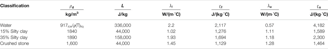

94% of researchers rate our articles as excellent or good
Learn more about the work of our research integrity team to safeguard the quality of each article we publish.
Find out more
ORIGINAL RESEARCH article
Front. Earth Sci., 10 November 2021
Sec. Cryospheric Sciences
Volume 9 - 2021 | https://doi.org/10.3389/feart.2021.733483
This article is part of the Research TopicEcological Impacts of Degrading PermafrostView all 19 articles
Water accumulation in permafrost regions causes a heavy thermal impact on the frozen layer, thereby leading to its degeneration. First, based on the real heat transfer process, this study proposes relevant hypotheses and governing equations for heat calculation models involving completely melted water, ice-bearing water, water–soil interface, and soil under water. The models consider the water surface as a thermal boundary on account of the natural buoyancy convection mechanism in water and the phase transition process. Second, this study verifies the accuracy of the calculation models regarding the measured water and permafrost temperatures. The four seasonal vertical temperature changes in the water according to this model are found to be consistent with the actual temperature-change trend, and the permafrost temperature under water is also consistent with the actual temperature field. This study thus provides theoretical support for the thermal impact analysis of water in permafrost regions.
The gradual expansion of construction works in permafrost regions of the Qinghai–Tibet Plateau has triggered several engineering problems, and in particular the accumulation of water along the roads. A field survey of the Qinghai–Tibet highway revealed that water accumulation along its sides has aggravated in recent years, that is, a tenfold increase in the number of ponds within 100 m of the highway on both sides from 2007 to 2009 (Jin et al., 2000; Lin et al., 2010; Luo et al., 2015; Xu and Wu, 2019). Such accumulation of water may exhibit a severe thermal impact on the permafrost in the surrounding areas, even leading to its melting (Karlsson et al., 2012; Kokelj and Jorgenson, 2013). In particular, the melting of permafrost with high ice content increases the depth of accumulated water and may even lead to thawing disasters in the surrounding regions (Langer et al., 2016). Thus, the most important effect of water accumulation on permafrost and its embankment is the thermal impact attributed to the special thermal sensitivity of permafrost (Calmels et al., 2008; Ling et al., 2012; Huang et al., 2013; Baranskaya et al., 2021). The permafrost suffers thermal erosion that results in decrease in the bearing capacity and stability of embankment, thereby causing uneven settlement, tumbling, or even cracking of the road surface (Niu et al., 2014; Wen et al., 2016; Lin et al., 2017; Sun et al., 2018). Hence, this study focuses on the effect of water accumulation on ground temperature and permafrost table change.
At present, the most important research on accumulated water in permafrost regions pertains to thermokarst lakes (Jorgenson et al., 2012). The main influence of these lakes on the environment and engineering works in permafrost regions is their thermal impact, which generally results in the conduction of vertical and lateral heat transfer to the surrounding permafrost. This transference can cause degradation of permafrost and decrease its stability (Hinkel et al., 2010; Kokelj et al., 2010; Samuelsson et al., 2010). The annual average ground temperature under a lake center is significantly higher in comparison to the temperature under a natural surface (Lin et al., 2011; Niu et al., 2011). This is mainly because a thermokarst lake can be a heat source and transfer energy to the surrounding permafrost, causing thermal erosion, and even transfer more heat downwards than the lateral transfer (Niu et al., 2018). This thermal erosion causes the permafrost under and around the lake to thaw, generating a gradually growing melting zone, and shows degradation effects such as temperature rise and decrease in the permafrost table (Pan et al., 2014; Wang et al., 2017; You et al., 2017). Moreover, lake temperature has been studied as the dominant factor of thermal influence (Burn, 2002). Stepanenko (2005) analyzed the heat and water exchanges between accumulated water and soil and suggested that the temperature gradient of lake water is the main factor affecting the thermal diffusion, freezing, and thawing of the surrounding permafrost.
Fang and Stefan (1996) proposed an accumulated water modified model that takes into account the heat exchange between water and bottom sediments, showing that the bottom water temperature change can affect soil temperature to a depth of 10 m. Water depth and the water–soil contact field have been found to directly affect the influence and extent of external changes on soil temperature. Lin et al. (2011) used a two-dimensional calculation model to assess the heat flux density between a thermokarst lake and its embankment and found that the former causes lateral thermal erosion of the latter. In conclusion, the current thermal calculation models for water accumulation in permafrost regions generally regard the bottom of the accumulated water as the thermal boundary and neglect the heat transfer process inside the water body, despite its significance. In alpine and cold environments, as in permafrost areas, the relationship between water depth and its maximum freezing depth also impacts the degree to which the lower soil layer is affected by water heat, and the temperature at the bottom of the water determines the development of the lower permafrost melting zone (Romanovsk and Osterkamp, 2000; Jorgenson and Shur, 2007; Gao et al., 2017). In the case of completely frozen water, the long-term observed temperature at the bottom of the water will be below 0°C. However, when the water depth is greater than or equal to the freezing thickness, the water does not completely freeze in winter, or only the bottom is frozen at the end of the cold season, and the temperature of the underlying soil continues to be above 0°C. The long-term effects of the above two scenarios will also drive the soil layer at the bottom of the water to gradually form a thawing layer (Hinkel et al., 2007; Wang et al., 2014). Therefore, the depth of the water and heat transfer in it constitute imperatives that cannot be neglected.
Mainly, the research and analysis about thermokarst lakes in permafrost regions are qualitative; the research methods are either site-measured data analysis or numerical calculation models, and heat transfer processes in the accumulated water are ignored. Moreover, water accumulations in permafrost regions are not exclusive of thermokarst lakes, and a large number of them are non-thermal water bodies with shorter formation times. In addition, limitations due to actual conditions render it difficult to study the thermal influence of various types of accumulated water on permafrost using measured data. Thus, this study establishes a calculation model that considers the water surface as the thermal boundary, the natural buoyancy convection mechanism of water, and the phase change process of water and its surrounding permafrost. The accuracy and feasibility of this calculation model were further verified by measured field temperature data. Hence, this study extends theoretical support for research on the influence of accumulated water in permafrost regions.
The model calculation was based on the separate heat transfer characteristics of water, ice, and soil because of the heat transfer difference in different media. In addition, the phase transition process of water and soil was also considered in permafrost regions. The model medium distributions in water and soil are shown in Figure 1.
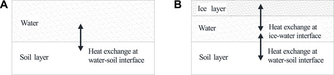
FIGURE 1. Model medium distribution. (A) Completely melted water body. (B) Water body with an ice layer.
In order to simplify the heat calculation of a completely melted water body in a permafrost region, the study considered the following assumptions:
1) The cross section of the accumulated water at different depths is equal.
2) Water is incompressible and isotropic, and mass exchange is regardless. The water density only depends on temperature.
3) The water temperature stratification is mainly reflected in vertical direction, and the heat exchange only occurs in vertical direction. Moreover, the water temperature in horizontal direction is equal.
4) Regardless of the external water supplement and heat exchange between the water surface and air caused by the wind speed, heat convection in the water body is only vertical natural buoyant convection caused by density difference.
As such, this study employed the equivalent heat conduction model based on the thermal diffusion theory, and the thermal diffusion coefficient in the traditional heat conduction equation represents the heat transfer caused by convection (Banimahd et al., 2013; Hondzo and Stefan, 2015). The heat transfer in accumulated water only occurs in vertical direction, and as such, using the theory of thermal diffusion, the convective heat transfer effect in vertical direction can be represented by thermal diffusivity in the model. Moreover, the governing equation of heat transfer in water can adopt the one-dimensional thermal diffusion equation (Banimahd and Zand-Parsa, 2013):
where Tw is the water temperature (°C); H is the depth of water (m);
where α is the coefficient determined by the degree of turbulence;
Accumulated water showed a phase change when the temperature drops below 0°C. This process is affected by meteorological factors, water temperature under the ice layer, and thermal characteristics of the ice layer. In order to calculate this phase change process in water body, the study considered the following assumptions:
1) There is no mass exchange with the external environment during the ice freezing and thawing process.
2) Ice layer freezes and thaws along vertical direction of water, and water body at the same depth freezes and thaws at the same time, and heat exchange only occurs in vertical direction.
3) The heat conduction process in the ice layer follows the Fourier thermal conductivity theory.
4) The water–ice conversion process is carried out in a small temperature range, −0.1–0°C.
5) The thermophysical parameters of the ice layer, such as specific heat capacity, thermal conductivity, and density, are all constant.
In this study, governing equations of the solid phase region and the liquid phase region were established based on the temperature method and the energy conservation theory. The governing equations of liquid accumulated water are described in Eq. 1. Besides, the governing equations in the solid phase, the ice layer, and water–ice interface equations are described as follows.
Governing equations in the ice layer (Fang et al., 1996) is given as follows:
The governing equation at the water–ice interface (Fang et al., 1996) is given as follows:
where
The heat exchange at the interface between accumulated water and lower soil affects the thermal state of the underlying permafrost, and as such the study considered the following assumptions: because the convective heat transfer between the bottom of the accumulated water and the lower soil is much smaller than heat transfer at the interface, so it is ignored. Therefore, it should be treated as a solid heat transfer problem.
Thus, the governing equation at the water–soil interface is (Shen, 2010) as follows:
where
Heat convection, mass migration, and other effects were neglected in the heat calculation of the permafrost under water, and in contrast, only the heat conduction of the soil and the phase change was considered. Assuming that the phase change of the aqueous medium in the model occurred in the temperature range (
where ρsoil is the density of soil (kg/m3); Csoil is the apparent specific heat of soil (J/(kg·°C));
First, in this experimental study, the researchers determined the water surface boundary of the model according to the thermal condition of the monitoring site. Then according to the control equation mentioned in The Governing Equation and Theoretical Model, the thermal calculation model for the permafrost with accumulated water was established considering the heat transfer process inside water. Finally, the reliability and feasibility of the model were verified by natural ground temperature, water temperature, and ground temperature under water at the monitored site.
Permafrost models without and with accumulated water were calculated in the study at this stage. The former verified the rationality of the calculation method by comparing it with the natural ground temperature of the monitoring site, whereas the latter verified the rationality and feasibility of the model, considering the interaction between the accumulated water and the permafrost. The soil layer distributions in the models were inferred to be consistent with that of the monitoring field, which is located near the Gonghe–Yushu expressway in the Qinghai–Tibet Plateau of China, shown in Figure 2. In the monitoring field, permafrost was observed to be a well-developed, mainly ice-rich permafrost, and soil–ice layer. The permafrost table of natural ground is about −0.8 to −3.5 m, the thickness of permafrost is about 60–100 m, and the annual average temperature of permafrost is about −2.0 to −1.5°C. Silty clay with an ice content of 15% distributes in −3 m of the upper layer, silty clay with ice content of 35% distributes in −3 m to −20 m, and gravel silty clay locates below −20 m.
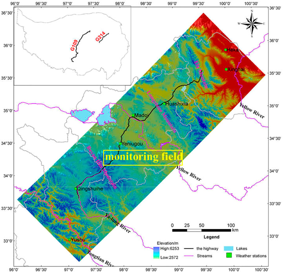
FIGURE 2. Location of monitoring field.
The size of the thermokarst lake in the monitored field is 40 × 50 m, and its maximum depth is 1 m. The monitoring time within which the study was conducted was from November 2013 to March 2015. During this time, the average air temperature was about −2.5°C, and the average annual cumulative precipitation was about 374 mm. The lowest temperature and highest temperature in a year usually occur in January and July, respectively. The measured temperatures of natural ground and lake center in the monitoring site were used for model verification. The probes were arranged in the same position for monitoring the temperature of the natural ground and lake center. The probes were arranged at −0.2, −0.5, −1.0, −1.5, −2.0, −2.5, −3.0, −3.5, −4.0, −5.0, −6.0, −7.0, −8.0, −10, −12, −14, −16, −18, and −20.0 m. The maximum depth of thaw in the natural ground and lake bottom was about −3.2 and −14 m in 2014. The temperature probe was installed in a steel pipe of 40 mm diameter, and the temperature measured in the steel pipe was regarded as the temperature of soil and water at the corresponding depth. The measurement accuracy and the resolution of temperature probe were ±0.05 and 0.01°C, respectively.
The geometric calculation model and the soil layer distribution are shown in Figure 3, and the corresponding thermal parameters are shown in Table 1. These thermal parameters were obtained from the reference Cao (2015). The soil depth was set to 60 m, and the water depth was set to 1 m, which is the same as the maximum depth of the measured thermokarst lake. The vertical and horizontal dimension of model geometry was 60 and 0.01 m. For the model of permafrost with accumulated water, the depth of water was 1 m and the depth of soil was 59 m under water in the vertical direction. The finite differential method was used for discretization calculation, and the difference between the calculation results of adjacent time steps was used as the accurate judgment. Time step was set to 1 h and, notably, the spin-up setting was different for the natural ground model and accumulated water model. For the natural ground model, geothermal gradient was obtained through the initial steady state calculation, and then the instant state was calculated for 300 years in order to obtain the initial temperature field. For the model of permafrost with accumulated water, the calculation method of the initial ground temperature field was the same as the natural ground model. After obtaining the initial ground temperature field, the accumulated water area was activated, and the initial temperature of the water was set to 4°C, which constituted the initial water temperature field.
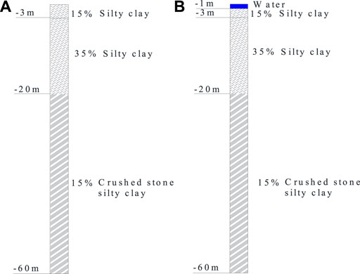
FIGURE 3. Geometric diagram and soil distribution of calculation models. (A) Natural ground. (B) Permafrost with accumulated water.
For the simulation of the monitoring site, true temperature boundary conditions are very important. The temperature data of the Madoi meteorological station were applied because there is no weather station at the monitored site. Based on the theory that when the altitude increases by 100 m, the temperature decreases by 0.6°C; the boundary layer theory, the air temperature and ground surface boundary of the monitored site were obtained as shown in Eqs. 12, 15–18. The temperature boundary of the monitored site water surface such as Eq. 13 was obtained based on the air temperature conditions and the measured data of the water surface temperature (Luo et al., 2016). The air temperature of the Madoi meteorological station is presented in the following equation:
where T0 is the initial annual average temperature (°C); c is the average annual temperature change rate (°C/s), a constant, determined by the temperature change trend of the Madoi meteorological station; t is the calculation time corresponding to the temperature change rate segment (s); A is the annual temperature amplitude (°C), according to the temperature record data of the Madoi meteorological station in the past 60 years (Figure 4), A = 12; ω is the constant that determines the function period, generally taken as 2π; and
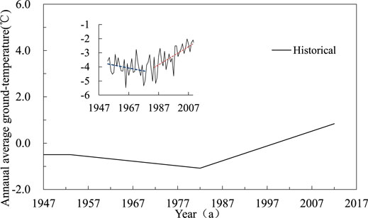
FIGURE 4. Temperature changes in Madoi from 1947 to 2014.
Based on the measured water surface temperature and the air temperature, the empirical formula for water surface temperature as a function of air temperature is fitted, as follows:
where
Taking π as the initial phase of temperature field calculations, from the previous periodic function of air temperature in Eq. 12, it can be seen that the calculation boundary starts from October 1 every year, so the initial water temperature was set as 4°C as per the measured average water temperature in October. The lower boundary always takes the constant heat flux of 0.0474 J/(m2·s) at the depth of −60 m (Cao, 2015), and the rest of the boundary is adiabatic.
The calculation accuracy of the natural ground model can be verified by measured data of the permafrost table, the permafrost thickness, and the ground temperature at a depth of −15 m, and, the calculation accuracy of the accumulated water model can be determined by measured data of the water and ground temperature changes and the thawing depth of permafrost under the water. As such, model verification is primarily divided into two parts. The acceptable calculation error of numerical simulation is 2–3°C (Banimahd and Zand-Parsa, 2013). Moreover, the Nash coefficient was also used to evaluate the model as follows:
where E is the Nash coefficient. When the value of E is closer to 1, the model reliability is higher. T is the calculation time (s);
1) Natural ground model
Combined with local temperature and permafrost conditions, the initial steady state was inferred as follows:
Instant state 300a is calculated to obtain the initial temperature field, and a is the abbreviation of annual, so 300a means 300 years.
According to the air temperature trend of Madoi, the calculation should be divided into three parts. Instant state 33a from 1914 to 1946 is shown as Eq. 17. Because recording of temperature data of the Madoi weather station began in 1947, the calculation period did not consider the change of annual average temperature.
Instant state 35a from 1947 to 1981 is as follows:
Instant state 33a from 1982 to 2014 is as follows:
The comparison of simulated and measured ground temperature is shown in Figure 5, which indicates that the simulated results are consistent with the measured data. For example, the figure shows that the calculated permafrost table on October 1, 2014, is about −2.6 m, which is similar to the permafrost table measure of −2.7 m at the monitored site. The permafrost thickness simulated at this time is almost the same as the actual permafrost thickness, both are about 17 m. The simulation and the measured permafrost temperatures demonstrate the same change trend along with the depth, and the annual average ground temperature of −15 m is −1.27°C and −1.30°C, respectively, and the Nash coefficient of permafrost temperature at the depth of −15 m is 0.71. Therefore, it can be safely inferred that the numerical simulation is in good agreement with the measured data, and it is optimally reflective of the law of the ground temperature change of permafrost at the monitored site, thereby indicating the robust feasibility of this simulation method.
2) Accumulated water model
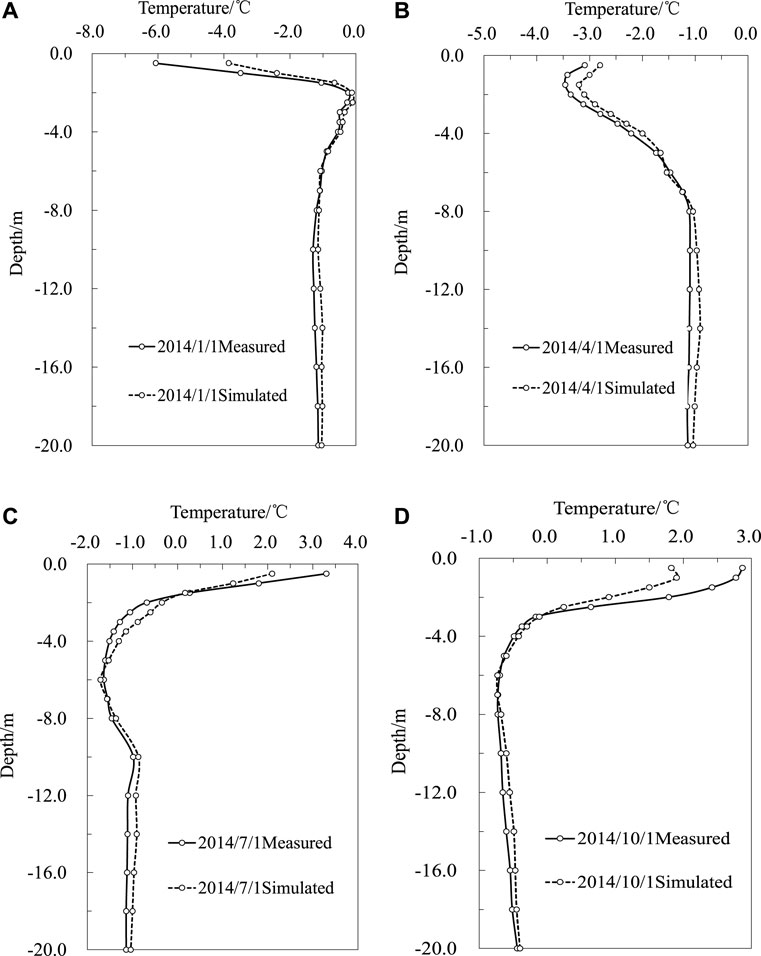
FIGURE 5. Comparisons of ground temperature between the monitored and the simulated. (A) January. (B) April. (C) July. (D) October.
The permafrost model was used before the accumulation of water, and the calculated frozen ground temperature was used as the initial temperature field of the permafrost part in the interaction model of accumulated water and the permafrost. Because the calculation start time was set as October 1, according to the actual measured water temperature in October, the initial water temperature in the calculation of the accumulation water was set to 4°C. For the calculation models, the ground and water surface boundary conditions were altered and suitably modified with time, as follows:
Instant state 300a is calculated to obtain the initial temperature field before the existence of accumulated water as follows:
Calculation of water temperature should be divided into three parts when accumulated water exists. Instant state 33a from 1914 to 1946 is presented in Eq. 22. Because recording of temperature data of the Madoi weather station began in 1947, the calculation period did not consider the change of annual average temperature.
Instant state 35a from 1947 to 1981 is presented in Eq. 23. The temperature data from the Madoi meteorological station show that the annual temperature experienced a small drop during the said period, and the temperature drop rate was −0.016°C/a, so the annual average temperature change is considered.
Instant 33a from 1982 to 2014 is presented in Eq. 24. The temperature rise rate during this period was 0.065°C/a.
Figure 6 shows the comparison of average water temperature between the measured water and the simulated one in 2014. The simulated water temperature was found to be consistent with the measured water temperature variation, and as such, the model reflects the actual variation of water temperature. Moreover, the difference between the simulated and actual values at each measured depth was less than 2°C. This calculation is based on the acceptable calculation error of the numerical simulation proposed by Banimahd and Zand-Parsa (2013), which is 2–3°C, and the Nash coefficient of water temperature at the depth of −1 m is 0.79. Therefore, it is considered that this calculation method can constitute a reliable computation to consider the accumulated water temperature change in the permafrost region.
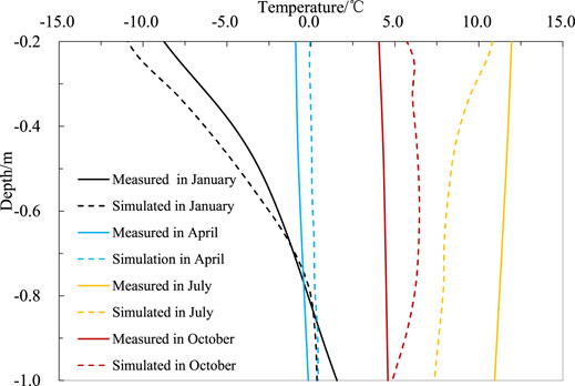
FIGURE 6. Contrast of water temperature law (1, 4, 7, and 10) in 2014.
Figure 7 shows the variation of permafrost temperature under the accumulated water in 5 years (1914, 1934, 1964, 2004, and 2014). It shows that the thawing depth of the permafrost gradually increases under the accumulated water along with the ground temperature rising. The average declining rate of the thawing depth was about 0.16 m/a before 1934, about 0.08 m/a from 1934 to 1964, and about 0.04 m/a from 1934 to 2014. The decrease of the maximum thawing depth of the lower permafrost gradually weakened, which can be essentially attributed to the increase in soil temperature. The temperature difference between the water bottom temperature and the lower soil temperature gradually decreased with time, and the amount of heat exchange between water and permafrost decreased, correspondingly weakening the thermal influence of water. Figure 7 also shows that the thermal transmission from the accumulated water caused a melting interlayer in the permafrost. The permafrost development is in conformance with the actual degradation phenomenon.
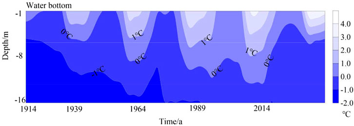
FIGURE 7. Variations of ground temperature under the accumulated water in years 1914, 1939, 1964, 1989, and 2014 during the calculation time.
The ground temperatures under the accumulated water increased by about 0.8°C at −15 m in the past 100a. Compared with the natural ground temperature of 2014 in Figure 5, the low-temperature permafrost under the accumulated water degenerated into extremely high-temperature permafrost. Considering that the thawing interlayer formed after 90 years of water accumulation, as shown in Figure 7, it is consistent with the development rule of the thermokarst lake (Luo et al., 2015). Moreover, the permafrost table and the variation of ground temperature under accumulated water also meet the thermal erosion characteristics of thermokarst lake (Peng et al., 2020). Therefore, this heat calculation model can be safely used in research and analysis of the thermal influence of accumulated water, and even thermokarst lakes, on permafrost.
Figure 8 shows the variation of the maximum thawing depth of the permafrost under the natural ground and the accumulated water in a calculation time of 100 years. It can be seen from this figure that the permafrost table under the accumulated water is decreasing year by year. The change rate of the permafrost table over time was initially rapid; however, it subsequently slowed down, varying from −3 to −14 m. Therefore, the findings indicate that the accumulated water can cause permafrost degradation.
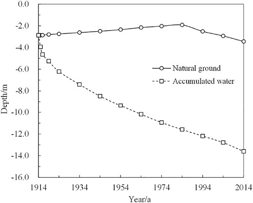
FIGURE 8. Comparison of the thaw depth for the natural ground and the permafrost underlying accumulated water body during the calculation time.
The comparison of the measured and simulated values of the permafrost temperature under the thermokarst lake in 2014 is shown in Figure 9. The Nash coefficient of permafrost temperature at the depth of −15 m was 0.68. Moreover, notably, the numerical simulation is in good agreement with the measured data and well reflects the change law and development trend of the permafrost temperature under water in the monitoring site. In addition, there was a melted interlayer with a thickness of about 13 m under the water. Under the simulation and measurement, the average annual ground temperatures were at −15 m are −0.18 and −0.20°C, respectively. The temperature at the interface between thermokarst lake water and permafrost showed seasonal changes. The temperature change trend is studied to be similar to the air temperature change at the site, and it was the highest in July and the lowest in April, in the study period. However, the amplitude at this interface was smaller than that of the air. It is because the specific heat of water is higher. Moreover, the average value of annual temperature at this interface is larger than that of air because water can accumulate heat in it. Therefore, the thermal calculation of the model between water and permafrost in permafrost regions is feasible and reliable.
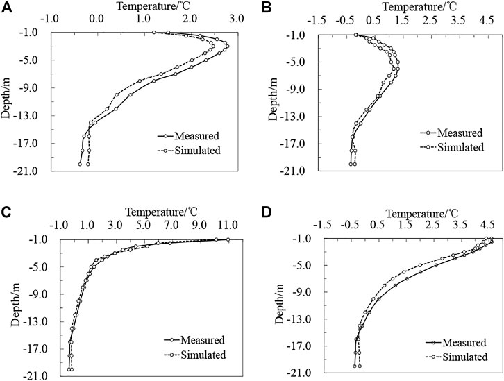
FIGURE 9. Comparison of the measured and simulated values of the permafrost temperature under the thermokarst lake water in January, April, July, and October, 2014. (A) January. (B) April. (C) July. (D) October.
The equivalent heat conduction model calculation method offers a robust inference regarding the characteristics of water temperature change within a year. Also, the heat transfer effect formed by the buoyant flow caused by the density difference is directly expressed by the change of water thermal conductivity. In addition, the number of calculation equations is reduced, which improves the convergence speed of the calculation. Therefore, the equivalent heat conduction model is sufficient to meet the calculation need, wherein the calculation speed is faster, and is deemed more suitable for the accumulation of water on permafrost.
The thermal erosion of permafrost from accumulated water increases the ground temperature and reduces the thickness of permafrost. The change of temperature at the interface between water and soil is consistent with the air temperature, but the amplitude is smaller. The accumulated water can cause permafrost degradation, even forming a melting interlayer.
The degree of the thermal impact of accumulated water on the underlying permafrost demonstrates an association with the changes in the external climate. The thermal impact in the early stage of water accumulation is found to be greater. As the permafrost table decreases, and the temperature difference between water and permafrost underlying decreases, consequently, the thermal influence of accumulated water on the lower permafrost gradually weakens.
The original contributions presented in the study are included in the article/Supplementary Material; further inquiries can be directed to the corresponding author.
EP: writing–original draft preparation and methodology. XH: writing—reviewing and visualization. YS: conceptualization and supervision. FZ: writing—reviewing and editing. JW: writing—reviewing and editing. WC: methodology.
This work was funded by the National Natural Science Foundation of China (41901079, 41971093), Province Natural Science Foundation of Gansu Youth Fund (20JR5RA435), CAS Youth talent growth Fund (Y9510608), Hongliu Excellent Youth Project of Lanzhou University of Technology (062006) and Gansu University innovation Fund Project (2020A-026). The observations in field were supported by Beiluhe Observation and Research Station on Frozen Soil Engineering and Environment in Qinghai-Tibet Plateau, Northwest Institute of Eco-Environment and Resources, Chinese Academy of Sciences.
The authors declare that the research was conducted in the absence of any commercial or financial relationships that could be construed as a potential conflict of interest.
All claims expressed in this article are solely those of the authors and do not necessarily represent those of their affiliated organizations, or those of the publisher, the editors, and the reviewers. Any product that may be evaluated in this article, or claim that may be made by its manufacturer, is not guaranteed or endorsed by the publisher.
The Supplementary Material for this article can be found online at: https://www.frontiersin.org/articles/10.3389/feart.2021.733483/full#supplementary-material
Banimahd, S. A., and Zand-Parsa, S. (2013). Simulation of Evaporation, Coupled Liquid Water, Water Vapor and Heat Transport through the Soil Medium. Agric. Water Manage. 130, 168–177. doi:10.1016/j.agwat.2013.08.022
Baranskaya, A., Novikova, A., Shabanova, N., Belova, N., Maznev, S., Ogorodov, S., et al. (2021). The Role of Thermal Denudation in Erosion of Ice-Rich Permafrost Coasts in an Enclosed Bay (Gulf of Kruzenstern, Western Yamal, Russia). Front. Earth Sci. 8, 566227. doi:10.3389/feart.2020.566227
Burn, C. R. (2002). Tundra Lakes and Permafrost, Richards Island, Western Arctic Coast, Canada. Can. J. Earth Sci. 39 (8), 1281–1298. doi:10.1139/e02-035
Calmels, F., Delisle, G., and Allard, M. (2008). Internal Structure and the thermal and Hydrological Regime of a Typical Lithalsa: Significance for Permafrost Growth and Decay. Can. J. Earth Sci. 45 (1), 31–43. doi:10.1139/e07-068
Cao, Y.-B. (2015). Evolution and Engineering Geology Evaluation of Permafrost along Gonghe-Yushu Highway. Beijing: University of Chinese Academy of Sciences Press.
Fang, X., Ellis, C. R., and Stefan, H. G. (1996). Simulation and Observation of Ice Formation (Freeze-over) in a lake. Cold Regions Sci. Technol. 24 (2), 129–145. doi:10.1016/0165-232x(95)00022-4
Fang, X., and Stefan, H. G. (1996). Long-term lake Water Temperature and Ice Cover Simulations/measurements. Cold Regions Sci. Technol. 24 (3), 289–304. doi:10.1016/0165-232x(95)00019-8
Gao, Z., Niu, F., Wang, Y., Luo, J., and Lin, Z. (2017). Impact of a Thermokarst lake on the Soil Hydrological Properties in Permafrost Regions of the Qinghai-Tibet Plateau, China. Sci. Total Environ. 574, 751–759. doi:10.1016/j.scitotenv.2016.09.108
Hinkel, K. M., Frohn, R. C., Nelson, F. E., Eisner, W. R., and Beck, R. A. (2010). Morphometric and Spatial Analysis of Thaw Lakes and Drained Thaw lake Basins in the Western Arctic Coastal Plain, Alaska. Permafrost. Periglac. 16 (4), 327–341. doi:10.1002/ppp.532
Hinkel, K. M., Jones, B. M., Eisner, W. R., Cuomo, C. J., Beck, R. A., and Frohn, R. (2007). Methods to Assess Natural and Anthropogenic Thaw Lake Drainage on the Western Arctic Coastal Plain of Northern Alaska. J. Geophys. Res. 112 (F2), 1–9. doi:10.1029/2006jf000584
Hondzo, M., and Stefan, H. G. (2015). Lake Water Temperature Simulation Model. J. Hydraul. Eng. 119 (11), 1251–1273. doi:10.1061/(ASCE)0733-9429(1993)119:11(1251)
Huang, W., Han, H., Shi, L., Niu, F., Deng, Y., and Li, Z. (2013). Effective thermal Conductivity of Thermokarst lake Ice in Beiluhe Basin, Qinghai-Tibet Plateau. Cold Regions Sci. Technol. 85 (JAN.), 34–41. doi:10.1016/j.coldregions.2012.08.001
Jin, H., Li, S., Cheng, G., Shaoling, W., and Li, X. (2000). Permafrost and Climatic Change in China. Glob. Planet. Change 26 (4), 387–404. doi:10.1016/s0921-8181(00)00051-5
Jorgenson, M. T., Kanevskiy, M., Shur, Y., Osterkamp, T., Fortier, D., Cater, T., and Miller, P. (2012). “Thermokarst lake and Shore Fen Development in Boreal Alaska”, in Proceedings of the Tenth International Conference on Permafrost, Salekhard, Russia: The Northern Publisher.
Jorgenson, M. T., and Shur, Y. (2007). Evolution of Ponds and Basins in Northern Alaska and Discussion of the Thaw Pond Cycle. J. Geophys. Res. 9 (6), 441–446. doi:10.1029/2006jf000531
Karlsson, J. M., Lyon, S. W., and Destouni, G. (2012). Thermokarst lake, Hydrological Flow and Water Balance Indicators of Permafrost Change in Western Siberia. J. Hydrol. 464-465 (none), 459–466. doi:10.1016/j.jhydrol.2012.07.037
Kokelj, S. V., and Jorgenson, M. T. (2013). Advances in Thermokarst Research. Permafrost Periglac. Process. 24, 108–119. doi:10.1002/ppp.1779
Kokelj, S. V., Lantz, T. C., Kanigan, J., Smith, S. L., and Courts, R. (2010). Origin and Polycyclic Behaviour of Tundra Thaw Slumps, Mackenzie Delta Region, Northwest Territories, Canada. Permafrost. Periglac. Process. 20 (2), 173–184. doi:10.1002/ppp.642
Langer, M., Westermann, S., Boike, J., Kirillin, G., Grosse, G., Peng, S., et al. (2016). Rapid Degradation of Permafrost underneath Waterbodies in Tundra Landscapes-Toward a Representation of Thermokarst in Land Surface Models. J. Geophys. Res. Earth Surf. 121 (12), 2446–2470. doi:10.1002/2016jf003956
Lin, Z.-J., Niu, F.-J., Ge, J.-J., Wang, P., and Dong, Y.-H. (2010). Variation Characteristics of the Thawing Lake in Permafrost Regions of the Tibetan Plateau and Their Influence on the Thermal State of Permafrost. J. Glaciol. 32 (2), 341–350. doi:10.3724/SP.J.1231.2010.06586
Lin, Z.-J., Niu, F.-J., Xu, Z.-Y., Xu, J., and Wang, P. (2011). Thermal Regime of a Thermokarst Lake and its Influence on Permafrost, Beiluhe Basin, Qinghai-Tibet Plateau. Permafrost. Periglac. 21 (4), 315–324. doi:10.1002/ppp.692
Lin, Z. J., Niu, F. J., Fang, J. H., Luo, J., and Yin, G. A. (2017). Interannual Variations in the Hydrothermal Regime Around a Thermokarst lake in Beiluhe, Qinghai-Tibet Plateau. Geomorphology 276 (JAN.1), 16–26. doi:10.1016/j.geomorph.2016.09.035
Ling, F., Wu, Q., Zhang, T., and Niu, F. (2012). Modelling Open-Talik Formation and Permafrost Lateral Thaw under a Thermokarst Lake, Beiluhe Basin, Qinghai-Tibet Plateau. Permafrost Periglac. Process. 23 (4), 312–321. doi:10.1002/ppp.1754
Luo, D.-L., Jin, H.-J., Lu, L.-Z., and Zhou, J. (2016). Spatiotemporal Changes in Extreme Ground Surface Temperatures and the Relationship with Air Temperatures in the Three-River Source Regions during 1980–2013. Theor. Appl. Climatol. 123 (3-4), 885–897. doi:10.1007/s00704-015-1543-6
Luo, J., Niu, F., Lin, Z., Liu, M., and Yin, G. (2015). Thermokarst lake Changes between 1969 and 2010 in the Beilu River Basin, Qinghai-Tibet Plateau, China. Sci. Bull. 60 (5), 556–564. doi:10.1007/s11434-015-0730-2
Niu, F.-J., Lin, Z.-J., Liu, H., and Lu, J.-H. (2011). Characteristics of Thermokarst Lakes and Their Influence on Permafrost in Qinghai–Tibet Plateau. Geomorphology 132 (3), 222–233. doi:10.1016/j.geomorph.2011.05.011
Niu, F.-J., Luo, J., Lin, Z.-J., Liu, M.-H., and Yin, G.-A. (2014). Morphological Characteristics of Thermokarst Lakes along the Qinghai-Tibet Engineering Corridor. Arct. Antarct. Alp. Res. 46 (4)–303. doi:10.1657/1938-4246-46.4.963)
Niu, F.-J., Wang, W., Lin, Z.-J., and Luo, J. (2018). Study on Environmental and Hydrological Effects of Thermokarst Lakes in Permafrost Regions of the Qinghai-Tibet Plateau. Adv. Earth. Sci. 33 (4), 335–342. doi:10.11867/j.issn.1001-8166.2018.04.0335
Pan, X., You, Y., Roth, K., Guo, L., Wang, X., and Yu, Q. (2014). Mapping Permafrost Features that Influence the Hydrological Processes of a Thermokarst Lake on the Qinghai-Tibet Plateau, China. Permafrost Periglac. Process. 25 (1), 60–68. doi:10.1002/ppp.1797
Peng, E.-X., Sheng, Y., Hu, X.-Y., Wu, J.-C., and Cao, W. (2020). Thermal Effect of Thermokarst lake on the Permafrost under Embankment. Adv. Clim. Chang. Res. 12 (1), 76–82. doi:10.1016/j.accre.2020.10.002
Romanovsky, V. E., and Osterkamp, T. E. (2000). Effects of Unfrozen Water on Heat and Mass Transport Processes in the Active Layer and Permafrost. Permafrost Periglac. Process. 11 (3), 219–239. doi:10.1002/1099-1530(200007/09)11:3<219::aid-ppp352>3.0.co;2-7
Samuelsson, P., Kourzeneva, E., and Mironov, D. (2010). The Impact of Lakes on the European Climate as Stimulated by a Regional Climate Model. Boreal. Environ. Res. 15 (2), 113–129. doi:10.1016/j.apcata.2010.02.027
Shen, H. T. (2010). Mathematical Modeling of River Ice Processes. Cold Regions Sci. Technol. 62 (1), 3–13. doi:10.1016/j.coldregions.2010.02.007
Stepanenko, V. M. (2005). Numerical Modeling of Heat and Moisture Transfer Processes in a System lake – Soil. Russ. Meteorol. Hydro. 3, 95–104.
Subin, Z. M., Riley, W. J., and Mironov, D. (2012). An Improved lake Model for Climate Simulations: Model Structure, Evaluation, and Sensitivity Analyses in CESM1. J. Adv. Model. Earth. Sy. 4 (1). doi:10.1029/2011ms000072
Sun, Z.-Z., Ma, W., Zhang, S.-J., Mu, Y.-H., Yun, H.-B., and Wang, H.-L. (2018). Characteristics of Thawed Interlayer and its Effect on Embankment Settlement along the Qinghai-Tibet Railway in Permafrost Regions. J. Mt. Sci-engl. 15 (005), 1090–1100. doi:10.1007/s11629-017-4643-1
Wang, H., Liu, H., and Ni, W. (2017). Factors Influencing Thermokarst lake Development in Beiluhe basin, the Qinghai-Tibet Plateau. Environ. Earth. Sci. 76 (24), 816. doi:10.1007/s12665-017-7143-2
Wang, Y.-B., Gao, Z.-Y., Wen, J., Liu, G.-H., Geng, D., and Li, X.-B. (2014). Effect of a Thermokarst lake on Soil Physical Properties and Infiltration Processes in the Permafrost Region of the Qinghai-Tibet Plateau. China. Sci. China. 57 (010), 2357–2365. doi:10.1007/s11430-014-4906-4
Wen, Z., Yang, Z., Yu, Q., Wang, D., Ma, W., Niu, F., et al. (2016). Modeling Thermokarst lake Expansion on the Qinghai-Tibetan Plateau and its thermal Effects by the Moving Mesh Method. Cold Regions Sci. Technol. 121, 84–92. doi:10.1016/j.coldregions.2015.10.012
Xu, X.-M., and Wu, Q.-B. (2019). Impact of Climate Change on Allowable Bearing Capacity on the Qinghai-Tibetan Plateau. Adv. Clim. Change Res. 10 (2), 99–108. doi:10.1016/j.accre.2019.06.003
Xu, X.-Z., Wang, J.-C., and Zhang, L.-X. (2001). Physics of Frozen Soil. Beijing: Science Publish House.
You, Y., Yu, Q., Pan, X., Wang, X., Guo, L., and Wu, Q. (2017). Thermal Effects of Lateral Supra-permafrost Water Flow Around a Thermokarst lake on the Qinghai-Tibet Plateau. Hydrol. Process. 31 (13), 2429–2437. doi:10.1002/hyp.11193
Zhang, M., Min, K.-H., Wu, Q., Zhang, J., and Harbor, J. (2012). A New Method to Determine the Upper Boundary Condition for a Permafrost Thermal Model: An Example from the Qinghai-Tibet Plateau. Permafrost Periglac. Process. 23 (4), 301–311. doi:10.1002/ppp.1755
Keywords: accumulated water, permafrost, ground temperature, thermal impact, calculation model
Citation: Peng E, Hu X, Sheng Y, Zhou F, Wu J and Cao W (2021) Establishment and Verification of a Thermal Calculation Model Considering Internal Heat Transfer of Accumulated Water in Permafrost Regions. Front. Earth Sci. 9:733483. doi: 10.3389/feart.2021.733483
Received: 30 June 2021; Accepted: 30 September 2021;
Published: 10 November 2021.
Edited by:
Huijun Jin, Northeast Forestry University, Harbin, ChinaReviewed by:
Bin Cao, Institute of Tibetan Plateau Research (CAS), ChinaCopyright © 2021 Peng, Hu, Sheng, Zhou, Wu and Cao. This is an open-access article distributed under the terms of the Creative Commons Attribution License (CC BY). The use, distribution or reproduction in other forums is permitted, provided the original author(s) and the copyright owner(s) are credited and that the original publication in this journal is cited, in accordance with accepted academic practice. No use, distribution or reproduction is permitted which does not comply with these terms.
*Correspondence: Xiaoying Hu, eGlhb3lpbmdodUBsemIuYWMuY24=
Disclaimer: All claims expressed in this article are solely those of the authors and do not necessarily represent those of their affiliated organizations, or those of the publisher, the editors and the reviewers. Any product that may be evaluated in this article or claim that may be made by its manufacturer is not guaranteed or endorsed by the publisher.
Research integrity at Frontiers
Learn more about the work of our research integrity team to safeguard the quality of each article we publish.