Wind Speed Forecasting in Fishing Harbor Anchorage Using a Novel Deep Convolutional Neural Network

Wind speed forecasting is an important issue in Marine fisheries. Improving the accuracy of wind speed forecasting is helpful to reduce the loss of fishery economy caused by strong wind. This paper proposes a wind speed forecasting method for fishing harbor anchorage based on a novel deep convolutional neural network. By combining the actual monitoring data of the automatic weather station with the numerical weather prediction (NWP) products, the proposed method constructing a deep convolutional neural network was based wind speed forecasting model. The model includes a one-dimensional convolution module (1D-CM) and a two-dimensional convolution module (2D-CM), in which 1D-CM extracts the time series features of the meteorological data, and 2D-CM is used to mine the latent semantic information from the outputs of 1D-CM. In order to alleviate the overfitting problem of the model, the L2 regularization and the dropout strategies are adopted in the training process, which improves the generalization of the model with higher reliability for wind speed prediction. Simulation experiments were carried out, using the 2016 wind speed and related meteorological data of a sheltered anchorage in Xiangshan, Ningbo, China. The results showed that, for wind speed forecast in the next 1 h, the proposed method outperform the traditional methods in terms of prediction accuracy; the mean absolute error (MAE) and the mean absolute percentage error (MAPE) of the proposed method are 0.3945 m/s and 5.71%, respectively.

Introduction

In the coastal areas of China, marine resources are abundant, and the local economic development mainly depends on fishing, marine transportation, marine oil, gas industry, etc. The rapid development of the marine economy brings prosperity to the local economy, but it also brings a number of safety issues, especially for small- and medium-sized fishing boats and fishermen who need shelter from strong winds. Statistics show that the majority of fishing boat windstorm accidents occur near ports, accounting for 68% of all fishing boat windstorm accidents, which is not only related to the delay in taking shelter from the wind but also related to the level of sheltered anchorage chosen by fishing boats. When the actual wind speed is greater than the wind resistance in the harbor anchorage, there is a risk of damage to the fishing vessel and loss of life to the crew. Besides, the large-scale integration of wind power and power grid requires accurate short-term wind speed prediction, especially for power system transmission and distribution planning, stability, reliability and safety prediction.

In the literature, many wind speed-forecasting approaches have been proposed to obtain reliable forecasts. Basic wind speed forecast methods are categorized into three classes, which consist of physical, statistical, and machine learning methods (Li et al., 2020). In the physical methods, most adoption is based on numerical weather prediction (NWP) and spatial correlation method (Buhan et al., 2017). These methods take full advantage of the physical properties of wind speed, and they usually require the use of detailed information such as low-level atmospheric physical information and local terrain to establish a fluid dynamics mode. The main disadvantage of physical methods lies in the high computational complexity, which needs continuous computing hours on a supercomputer (Shokrzadeh et al., 2017).

The statistical methods are the persistence method, Kalman filter, autoregressive moving average (ARMA) method, etc. (Erdem and Shi, 2011). Among them, the ARMA model is adopted most, mainly because it has low model complexity and flexible input. The idea of these models is to mine the relationship between the historical wind speed time series and the predicted wind speed, but the disadvantage is that the quality of data is required to be high, and the prediction accuracy will decline with the increase in the prediction time (Colak et al., 2012). Machine learning method is also strictly a statistical method, such as the wind speed prediction method based on support vector regression (SVR) proposed in the literature (Huan et al., 2018), artificial neural network (ANN) in the literature (Azad et al., 2014), and the extreme learning machine (ELM) method in the literature (Liu et al., 2018), these traditional machine learning models tend to learn the abstract features of the shallow layer, which makes it difficult to further improve the accuracy of wind speed prediction.

With the rapid development of deep learning, the model based on deep neural network is better than that based on shallow model in feature extraction, and can improve the accuracy of wind speed prediction (Khodayar and Teshnehlab, 2016; Zhang et al., 2017; Khodayar et al., 2017). In order to improve the accuracy of wind speed prediction in fishing harbor anchorage, this paper proposes a wind speed prediction method based on convolutional neural network (CNN). The prediction model designed in this paper is composed of multilayer convolutional neural network and fully connected network, which not only uses one-dimensional convolutional neural network (1D-CNN) to extract the time series information of each meteorological parameter but also uses two-dimensional convolutional neural network (2D-CNN) to gradually mine the underlying deep abstract feature information in the original data, it provides effective depth characteristic data for regression layer. For the overfitting problem that is prone to occur in the model, L2 regularization constraint is added to the connection weight of each layer in the model, and dropout strategy is adopted for the neurons in each layer, so that a more robust prediction model can be trained. Finally, compared with other methods, the effectiveness of the proposed method for predicting wind speed in the next hour is verified by experiments.

Wind speed forecasting model

Model design

As shown in Figure 1, to effectively extract the time series features and depth abstract features in the wind speed prediction time series data, a wind speed prediction model structure with three convolutional layers is designed in this paper. In the figure, Conv denotes the convolutional layer, Max Pooling means the Pooling layer, and FC represents the full connection layer, where $\text{FC}\cdot 1\text{/sigmoid}$ represents that FC contains one unit of hidden layer, and sigmoid function is used as the activation function; $3\times 3\text{Conv}2\text{D}\cdot 64\text{/ReLu}$ means that convolution kernel of size is used in 2D convolutional layer, the number of which is 64, and ReLu function is used as the activation function; the rest of the graphic meanings are similar to those mentioned above.

FIGURE 1

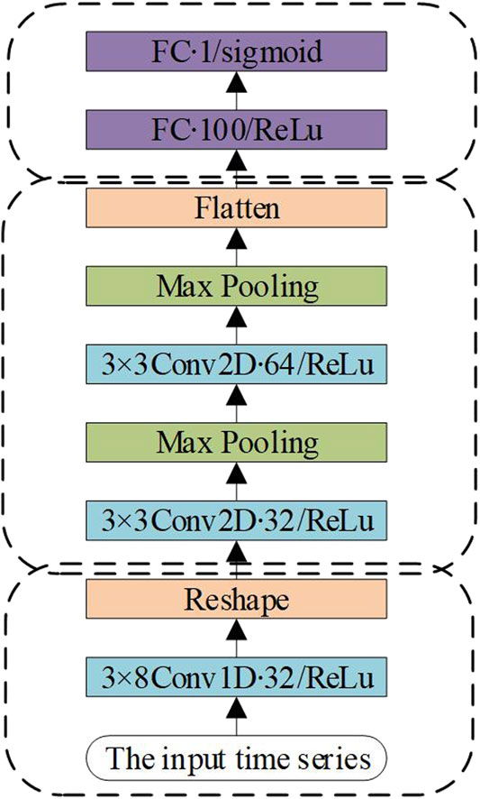
FIGURE 1. The structure of the proposed wind speed prediction model.

In this model, the input data are composed of a variety of meteorological parameter time series. After the model input construction, the characteristic graph of time series suitable for deep convolutional neural network model processing can be generated. The first layer of the model is a one-dimensional convolutional layer, which uses 32 convolutional kernels of size $3\times 8$ to extract timing features; we can get 32 channels of one-dimensional feature map, then the reshape layer is used to splice these one-dimensional feature maps into a new feature map. Next, for the feature map obtained from the previous layer, the depth abstract feature is extracted by the two-dimensional convolutional layer. In the first layer of 2D-CNN, 32 convolution kernels of size $3\times 3$ were adopted to obtain the 2D feature mapping of 32 channels. After the max pooling, the length and width of the 2D feature mapping were halved. In the second layer of 2D-CNN, the convolutional kernels of 2d-cnn and 2d-cnn in the first layer were the same size, but the number of convolutional kernels was expanded to twice the original size, and also, max pooling was used to sample the 2D feature maps. In order to compress the two-dimensional feature map of 64 channels into one dimension, the flatten layer is used. At this time, the extracted features were highly abstract, which was conducive to accurately express the behavior of dynamic changes of the future wind speed. Finally, the full connection layer of 100 hidden units is used to reduce the dimension of the one-dimensional feature of compression, and the fully connection hidden neural unit of a single output layer outputs the wind speed prediction results.

Model input construction

In addition to its autocorrelation, wind speed is also related to meteorological variables such as wind direction, temperature, and atmospheric pressure (Mahdi and Jianhui, 2018; Liang et al., 2018; Kingma and Ba, 2014). The input of the model in this paper adopts meteorological variables, such as wind speed, wind direction, temperature, relative humidity, dew point temperature, wind cooling index, precipitation, and atmospheric pressure. One part of the input data of the model is the measured data from the sensor of the meteorological automatic observation station, and the other part is the numerical weather prediction (NWP) data. NWP data are based on objective meteorological variable data. Under certain initial value and boundary setting conditions, the future weather can be predicted by numerical calculation. The introduction of NWP data not only enriches the input characteristic data but also makes up the shortcoming that the measured data cannot describe the future meteorological variable.

The deep convolutional neural network model proposed in this paper takes the time series feature maps as the input of the model, which is similar to the word vector representation method in natural language processing. The wind speed value at a certain time and various meteorological variables at the same time are connected in series to form a set of vectors, thus, forming a new time series unit. Then the time series unit, composed of the collected measured data and NWP data, is arranged in order of time; the measured and NWP data are intercepted, in turn, by means of a sliding window, and the intercepted data are combined into a feature map. The process of model input construction is shown in Figure 2.

FIGURE 2

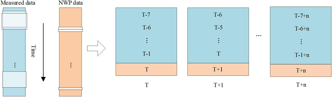
FIGURE 2. The process of model input construction.

As shown, the measured data of the sliding window size are $7\times 8$, the NWP data of the sliding window size are $1\times 8$, the sliding step length is set to 1, and the combined characteristics of the figure for the size is $8\times 8$, where, T is the specific time of a certain time, the time interval with the adjacent time is 1 h, and T + n is the future n 1-h intervals of time at time T. The label of each feature map is the true value of the wind speed at the predicted time.

The model details

The above content has given the basic structure of the proposed model and the construction method of the model input, and then the details of the model are elaborated:

One dimensional convolutional neural network: First, the model proposed adopts the 1D-CNN layer to process the input time series data. The 1D-CNN is a network structure that is good at processing the time series. Convolution operation can effectively extract the local information in the sequence signal, which has been widely applied in speech recognition, natural language processing, fault feature extraction, and other fields. Its basic structure is shown in Figure 3.

FIGURE 3

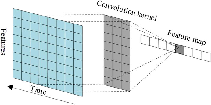
FIGURE 3. The basic structure of 1D-CNN.

Suppose the time series of the input is $\mathit{X}\in {\Re }^{s\times d}$, where $s$ is the time dimension and $d$ is the feature dimension; after one-dimensional convolution operation, the results of the time series data are as follows:

$a_c^j=f_r\left(\mathit{x}\ast {\mathit{W}}_c^j+b\right)(1)$

$f_r\left(z\right)=\max \left(z,0\right)(2)$

In the above formula, $a_c^j$ is the feature map obtained by the convolution kernel operation; $\mathit{x}$ is a subset of $\mathit{X}$, which is generated by the mapping during the sliding process of the convolution kernel, and its size is the same as ${\mathit{W}}_c^j$; $\ast$ represents the convolution operation; ${\mathit{W}}_c^j$ represents the convolution kernel, $j\in \left[1,n_c\right]$, where $n_c$ is the number of convolution kernels, and ${\mathit{W}}_c^j\in {\Re }^{m\times d}$. In this article, the value of m is set to 3, and b is the bias. $f_r\left(z\right)$ is the activation function. The activation function adopted here is the ReLu function.

Two-dimensional convolutional neural network: Compared with the one-dimensional convolutional neural network, the main characteristic of the two-dimensional convolutional neural network is that the computing direction of its convolutional kernel is 2D, which is a network structure suitable for processing picture information. After the time series data were processed by 1D-CNN, the one-dimensional feature map of multiple channels was obtained. By using the reshape layer, these one-dimensional feature maps are pieced together into a new feature map, which is a high abstraction of the characteristics of meteorological variables such as wind speed, temperature, precipitation, and atmospheric pressure in the original adjacent time. Next, the model uses the 2D-CNN layer to continue to mine the hidden feature information of the original input; the structure of 2D-CNN is shown in Figure 4.

FIGURE 4

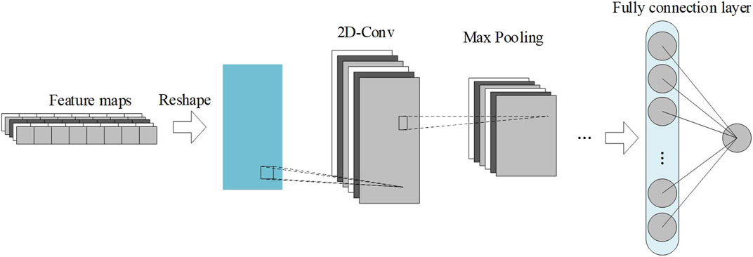
FIGURE 4. Architecture of 2D-CNN.

Suppose the input feature map is $\mathit{M}\in {\Re }^{n_c\times s}$, where $n_c$ is the number of convolution kernels in 1D-CNN layer, $s$ is the time dimension. After two-dimensional convolution operation, the result of feature map is:

$b_d^j=f_r\left(\mathit{m}\ast {\mathit{W}}_d^j+{\mathit{b}}^{\prime }\right)(3)$

In the formula Eq. 3: $b_d^j$ is the jth feature map obtained by the convolution kernel operation, $\mathit{m}$ is a subset of $\mathit{M}$, and it is generated by the mapping during the sliding process of the convolution kernel. Its size is the same as ${\mathit{W}}_d^j$, ${\mathit{W}}_d^j$, which represents the kernel of 2D-CNN, $j\in \left[1,n_d\right]$, where ${\mathit{W}}_d^j\in {\Re }^{3\times 3}$ is the convolution kernel of 2D-CNN, which is $\mathbf{3}\times \mathbf{3}$ with fixed size in this paper. The other parameters are similar to Eq. 1, so we will not give too much explanation here.

In addition to the two-dimensional convolutional layer, the 2D-CNN in this paper also includes max pooling. The use of maximum pooling sampling will not only reduce the parameters of the model but also extract more obvious abstract features for the wind speed prediction task, so that it can be better utilized by the subsequent network layer. The max pooling layer is defined by Eq. 4:

$h_d^j=f_r\left({\beta }_p\cdot \max \left(t\left(b_d^j\right)\right)+b_p\right)(4)$

In Eq. 4, $h_d^j$ is the maximum pooled output of the corresponding feature map $b_d^j$, the function $t(\cdot )$ represents the downsampling function, $\max (\cdot )$ means that the maximum value is selected from the sample value as the eigenvalue, ${\beta }_p$ is the multiplicative bias, and $b_p$ is the additive bias.

The last part of the 2D-CNN structure is the full connection layer, which further combines the global deep abstract features. The output results are as follows:

${\mathit{o}}_{\mathit{fc}}=f_r\left({\mathit{h}}_{\mathit{last}}\cdot {\mathit{W}}_{\mathbf{f}\mathbf{c}1}+{\mathit{b}}_{\mathbf{f}\mathbf{c}1}\right)(5)$

In Eq. 5: ${\mathit{h}}_{\mathit{last}}$ represents the vector flattened by the flatten layer, ${\mathit{W}}_{\mathrm{f}\mathrm{c}1}\in {\Re }^{n_{\mathrm{f}\mathrm{c}}}$ is the weight matrix of the full connection layer, and $n_{\mathit{fc}}$ is the number of hidden cells of the full connection layer; the activation function is also the ReLu function. For the final wind speed regression problem, the number of unit output is 1, and the output of the regression result is obtained through the full connection layer:

$\tilde{y}=f_{\sigma }\left({\mathit{o}}_{\mathit{fc}}\cdot {\mathit{W}}_{\mathbf{f}\mathbf{c}2}+{\mathit{b}}_{\mathbf{f}\mathbf{c}2}\right)(6)$

$f_{\sigma }\left(z\right)=\frac{1}{1+e^{-z}}(7)$

In Eqs. 6 and 7: $\tilde{y}$ represents the final regression prediction result, where the activation function $f_{\sigma }\left(z\right)$ is a sigmoid function.

Model training and strategy

In order to train the proposed model and deal with the task of predicting wind speed in the next hour, a set of training feature maps was constructed from the time series of the original meteorological parameters, feature maps $\left\{x_1,x_2,\cdots x_m\right\}$, where ${\mathit{x}}_i\in {\mathit{R}}^{8\times 8}$. The true wind speed label corresponding to the feature maps is $\left\{y_1,y_2,\cdots y_m\right\}$, the parameters $\left\{\mathit{W},\mathit{b},{\mathit{W}}_{\mathrm{f}\mathrm{c}},{\mathit{b}}_{\mathrm{f}\mathrm{c}}\right\}$ of the model were adjusted through supervised training, and the expression of the objective loss function to be minimized in the model is:

$J=\frac{1}{m}{\displaystyle \sum _{i=1}^{m}L\left(g\left({\mathit{x}}_{\mathit{i}},\mathit{W},\mathit{b},{\mathit{W}}_{\text{fc}},{\mathit{b}}_{\text{fc}}\right),y_i\right)}(8)$

$L={\left({\tilde{y}}_i-y_i\right)}^2(9)$

In Eq. 8, this function represents the mean square error function, where the contents of the function are simplified and expressed by formula Eq. 9, and $g(\cdot )$ represents the feature transformation function of the deep convolutional neural network, $\mathit{W},\mathit{b}$ represents the connection weight and bias of the convolutional layer in the 1D-CNN layer and 2D-CNN layer, and ${\mathit{W}}_{\mathrm{fc}},{\mathit{b}}_{\mathrm{fc}}$ represents the connection weight and bias in the fully connected layer.

In deep convolutional neural network, one of the biggest problems is prone to overfitting. In order to prevent this problem, regularization method can be used to strengthen the generalization ability of the model. In this paper, L2 norm is adopted to constrain the connection weight matrix of each layer, which can reduce the complexity of the model. The expression of the objective loss function minimized after L2 norm is adopted is:

$J=\frac{1}{m}{\displaystyle \sum _{i=1}^{m}L\left(g\left({\mathit{x}}_{\mathit{i}},\mathit{W},\mathit{b},{\mathit{W}}_{\text{fc}},{\mathit{b}}_{\text{fc}}\right),y_i\right)}+\frac{{\lambda }_1}{2}{\Vert \mathit{W}\Vert }_F^2+\frac{{\lambda }_2}{2}{\Vert {\mathit{W}}_{\text{fc}}\Vert }_F^2(10)$

In Eq. 10: the second and third terms represent the L2 regular terms, and ${\lambda }_1$ and ${\lambda }_2$ are the weight attenuation coefficients.

After the objective loss function is given, the backpropagation algorithm is used to train the entire deep convolutional neural network model and selects the Adam algorithm (Khodayar et al., 2017) as the gradient optimization algorithm of the model. The Adam algorithm shows the advantages of inertia retention and environment perception. The algorithm calculates the adaptive learning rate of different parameters from the first and second moment budgets of the gradient, the idea of calculating the mean value in sliding window is adopted for numerical fusion, and the contribution of the gradient to the current mean declines exponentially.

In addition to regularization, the dropout strategy can also be used to further prevent the occurrence of overfitting of the model. The dropout strategy is an optimization during network training. Hidden neurons in the network are randomly discarded according to a certain probability. During the training process, discarded neurons do not participate in forward and backpropagation, but their corresponding weights are retained. On the one hand, this operation can effectively reduce the number of internal parameters in the model; on the other hand, it increases the diversity of input data in the model and, to some extent, reduces the probability of the occurrence of overfitting phenomenon. The dropout technology diagram is shown in Figure 5 where ⊗ means the discarded part.

FIGURE 5

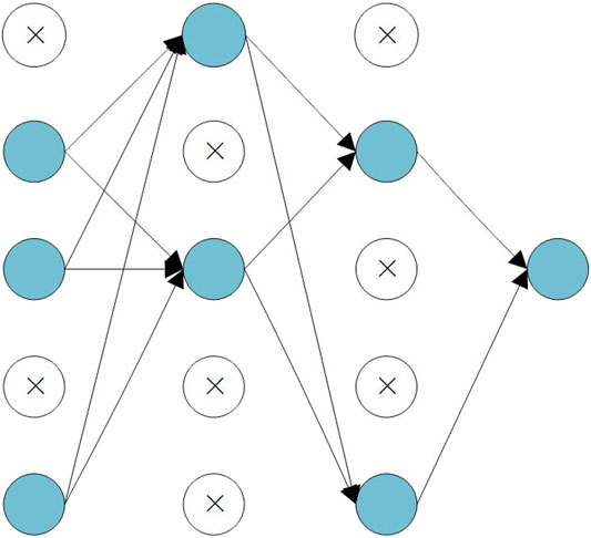
FIGURE 5. Dropout strategy schematic.

Experimental results

In this paper, the measured and NWP data of a harbor anchorage in Xiangshan, Ningbo, China, from January 1, 2016 to December 31, 2016, were used as experimental samples to verify the validity of the prediction model based on deep convolutional neural network, where the sampling interval of samples is 1 h. Due to the obvious seasonal characteristics of wind speed, five consecutive days in each season were randomly selected as the test period to verify the accuracy of this model in wind speed prediction and the experimental comparison with other traditional wind speed prediction models.

Error evaluation indexes

In order to comprehensively evaluate the predictive performance of the model, mean absolute error (MAE), mean absolute percentage error (MAPE), and root of the mean squared error (RMSE) were used as error evaluation indexes; the expressions of error indexes are as follows:

$\mathit{MAE}=\frac{1}{N}{\displaystyle \sum _{t=1}^N\left|y_t-{\widehat{y}}_t\right|}(11)$

$\mathit{MAPE}=\frac{1}{N}{\displaystyle \sum _{t=1}^N\left|\frac{y_t-{\widehat{y}}_t}{y_t}\right|}\times 100\%(12)$

$RMSE=\sqrt{\frac{1}{N}{\displaystyle \sum _{t=1}^N(y_t}-{\widehat{y}}_t{)}^2}(16)$

In the above formula: $y_t$ and ${\widehat{y}}_t$ represent the true value and the predicted value respectively, and $N$ is the total number of samples.

Experiment setup and training process

In this paper, in addition to being randomly selected from each season for 5 days as a test period, and to the rest of the samples according to the proportion of $9:1$, the samples were divided into the training set and validation set. In order to balance the characteristic parameters and reduce the computation and error of the model, the data need to be normalized. Then the input samples of the training model were established according to the model input construction, and 8,760 feature maps were generated, and the labels of each feature map were the real wind speed in the next hour. Finally, a total of 480 feature maps were used as the test set, 7,542 feature maps were used as the training set, and 828 feature maps were used as the validation set.

The super parameters of the proposed deep convolutional neural network model include the model structure, learning rate, and regular term coefficient. The model structure of this paper is the three-layer convolutional layer prediction model structure given in Figure 1; the learning rate was set to 0.03, no regular terms were used, and the number of iterations was set to 200. Iterative training was conducted on the proposed model, and the training process is shown in Figure 6A.

FIGURE 6

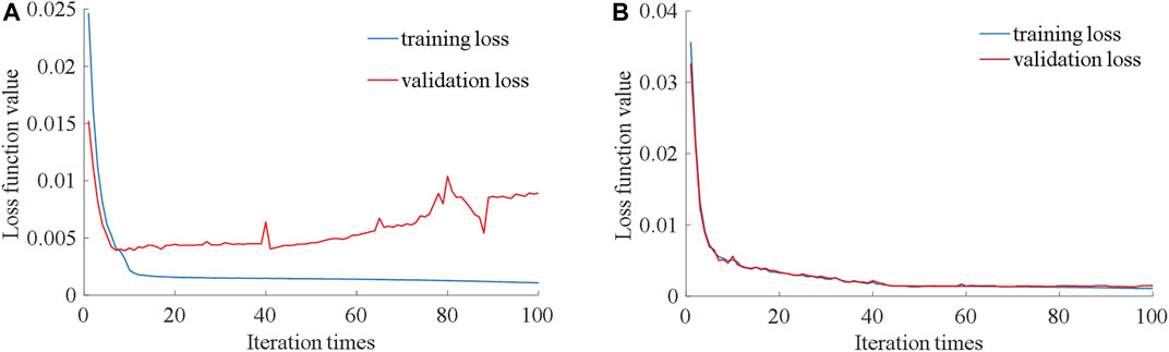
FIGURE 6. The curve of the loss function during the training of the model.

It can be seen from Figure 6A that the verification loss presents a gradually increasing trend with the increase in iteration times. At the end of the training process, the MAE of the training set for wind speed fitting reaches 0.3527 m/s, while the MAE of the verification set for wind speed prediction is 1.1461 m/s, indicating that the model generates an overfitting phenomenon after the training. Next, the model is improved by using the dropout strategy and L2 regularization constraint on all connection weights to enhance the generalization performance of the model. After a large number of experimental studies, when the dropout threshold is set to 0.2, and the L2 regular term coefficients ${\lambda }_1$ and ${\lambda }_2$ are set to 0.0005, the convergence of the model is better. The improved model training process is shown in Figure 6B. As can be seen from Figure 6B, with the increase in iteration times, the training loss and verification loss of the model decrease in step with each other, and the MAE of the two finally reaches is close to each other, about 0.3446 m/s.

Analysis of Convolutional Neural Network Structure

Next, in order to explain the rationality of the network structure of the proposed model, the control variable method is adopted to deepen the model structure of the 1D-CNN model and the proposed model step by step. The prediction effect of the different structure models was tested by deepening the 1D-CNN layer or 2D-CNN layer continuously, in which the regression prediction layer remained unchanged and remained the fully connected layer of the two-layer structure. Among them, the 1D-CNN model only uses the 1D-CNN layer as the feature extraction layer of the convolutional neural network. After extracting the temporal feature information with the 1D-CNN layer of the first layer, the proposed model uses the 2D-CNN layer of multiple layers to extract the deep abstract feature information. The prediction scatter diagram of the different models with different convolutional layer structures is shown in Figures 7 and 8.

FIGURE 7

FIGURE 7. Prediction scatter diagram of the different convolutional layer structures in the 1D-CNN model.

FIGURE 8

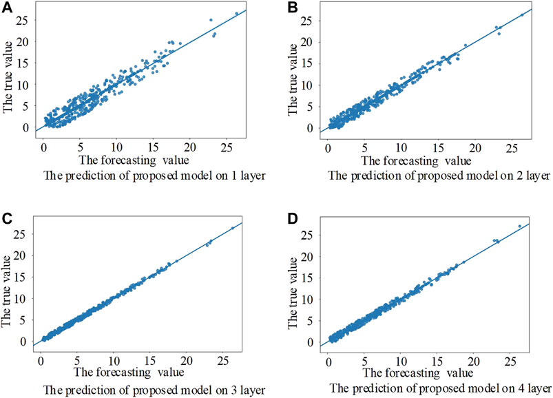
FIGURE 8. Prediction scatter diagram of the different convolutional layer structures of the model in this paper.

It can be seen from Figures 7 and 8 that the convolutional neural network model with a layer of 1D-CNN structure has possessed certain predictive power, but its error is bigger, still unable to accurately predict the change in wind speed, then gradually increasing the 1D-CNN layer or 2D-CNN layer, and the 1D-CNN model and the proposed model of wind speed forecasting error decreases. In this paper, the error of the proposed model increases when the 2D-CNN layer increases to the fourth layer, which, to some extent, indicates that the model is overlearning. The structure of the model can be determined through the above experiments. The prediction error histogram of the two models with different convolutional layer structures is shown in Figure 9.

FIGURE 9

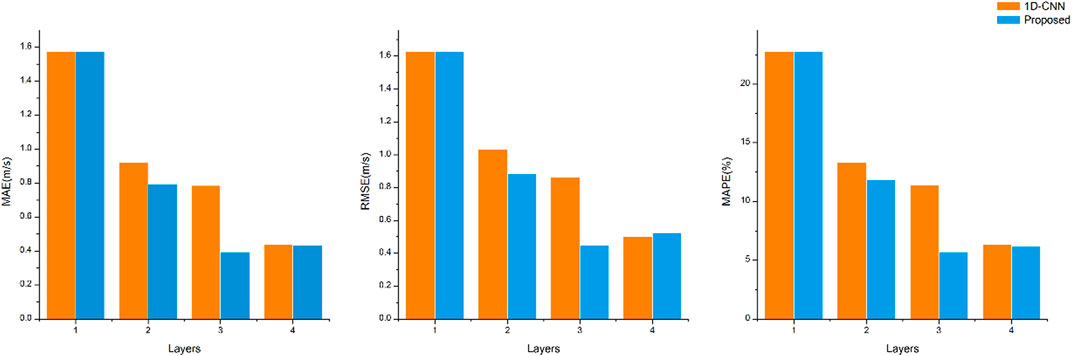
FIGURE 9. Histogram of the prediction error of the two models under different convolutional layer structures.

Comparisons of Different Models

In the model comparison experiment in this paper, the test set is derived from the random selection of consecutive 5 days in each season as the test period. In order to compare the prediction performance difference between the traditional wind speed prediction model and the proposed model, the persistence method, ARMA, SVR, DBN, LSTM, and 1D-CNN were selected as controls for wind speed prediction in the next hour.

As a benchmark model, the persistence method is the simplest wind speed prediction method, which takes the observed wind speed of the nearest point as the predicted value of the next point. This method is suitable for the prediction below 3∼6 h. The persistence method and the absolute error of the forecast results of the proposed method are given in Figure 10 and the absolute error distributions are given in Figure 11.

FIGURE 10

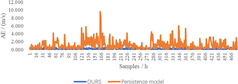
FIGURE 10. Comparison of the persistence method and ours.

FIGURE 11

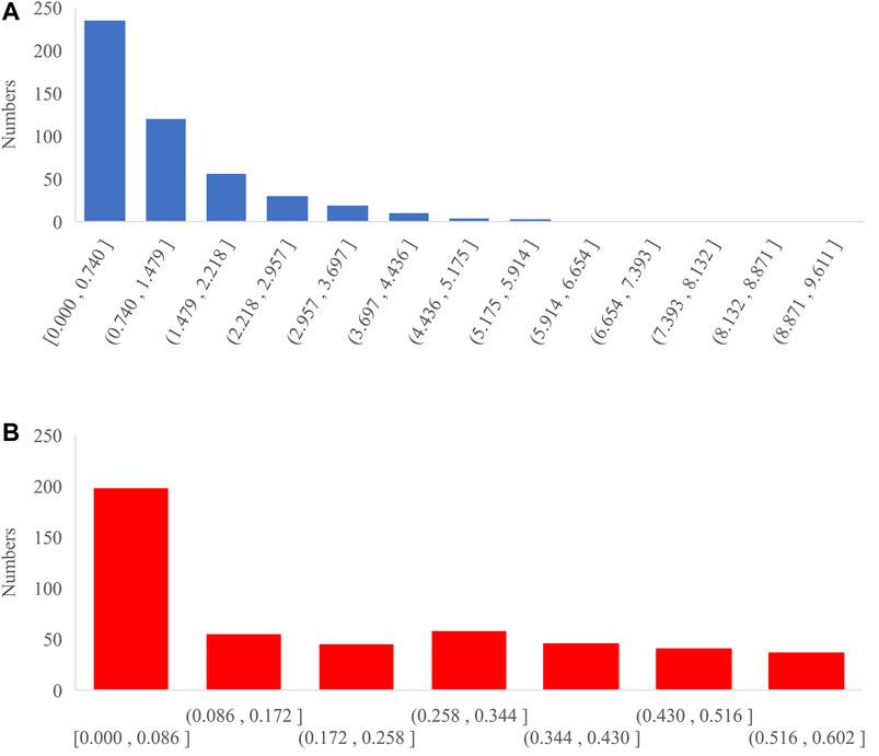
FIGURE 11. Absolute error distributions of the persistence model and ours. (A) Persistence model. (B) Ours.

It can be seen from Figure 10 that wind speed prediction of the persistence model fluctuates greatly, not stable, but from the AE distribution in Figure 11, the persistence model has relatively good prediction performance, and most of the absolute prediction errors are between 0 and 0.740 m/s. Through calculation and comparison, the mean and variance of the absolute error of the persistence model predicted value are 1.1307 and 1.3771, and the mean and variance of the absolute error of our predicted value are 0.3945 and 0.0368. It can, therefore, be concluded that the proposed model is more powerful than the persistence model.

Next, comparative experiments were conducted with other models. In the ARMA model, the wind speed series data are smoothed first; after parameter tuning, the parameter p of the autoregression part is 3, and the parameter q of the moving average part is 2. The SVR uses the Gaussian kernel function, and its parameter penalty factor C and control radius $\delta$ are set to 187.6 and 0.1203, respectively, after parameter tuning. In the DBN model, the structure of the hidden layer and hidden unit of the model is adjusted, and the structure with the best prediction performance is $\left[\mathrm{400,200,150,50,1}\right]$. However, in the LSTM model, the structure with the best predicted performance is $\left[\mathrm{200,100,10}\right]$ after the structural parameter tuning of the model. Finally, the wind speed prediction results of the different prediction models for the next 1 h during the test period are shown in Figure 10, and the absolute errors between predicted samples and real samples of the different models are shown in Figure 11.

As can be seen from Figure 12, when the wind speed is large and fluctuates relatively, the predicted value of wind speed of the above five models is close to the real value, and all of them can predict the change in wind speed more accurately, as shown in the figure. However, when the wind speed is small, or the fluctuation range is large, the prediction deviation of model 1D-CNN and the model proposed in this paper is smaller than that of the other models. Since the convolutional neural network builds dense features through mining and is more sensitive to changes in input features than other models, model 1D-CNN and the model in this paper can achieve more accurate prediction results. It can be seen from the absolute errors of the different models in Figure 13 that the overall error of the proposed model is relatively small. The predictions of other models have large fluctuations and present an unstable state, especially in the predictions of individual sample points, which have large deviations. The error results, training, and prediction time of the six models for predicting the wind speed in the next hour are shown in Table 1. All models are run on a personal computer with 3.07-GHz i7 CPU and 16-GB RAM. Except for the ARMA model, which only uses wind speed data, all other models use the same dataset.

FIGURE 12

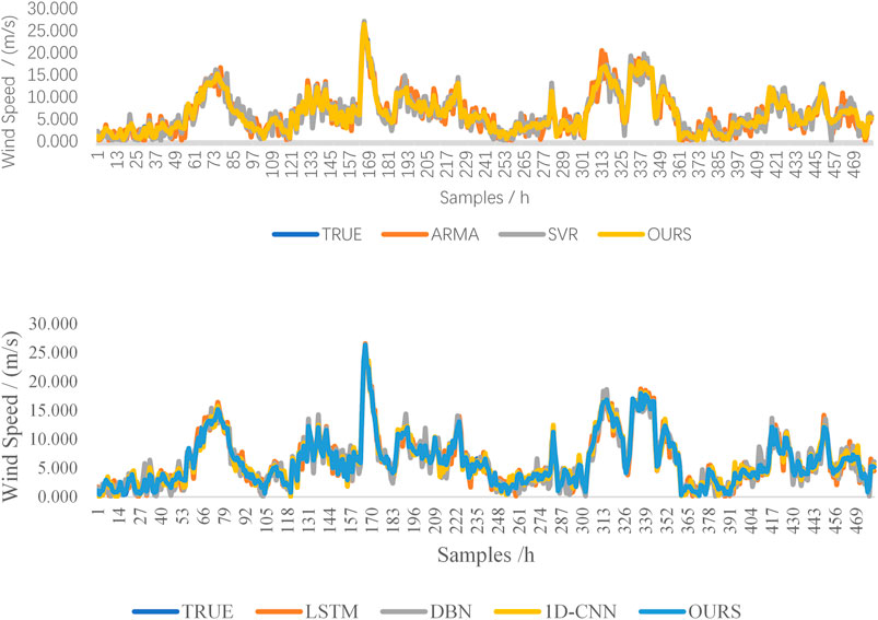
FIGURE 12. Prediction results of the different models.

FIGURE 13

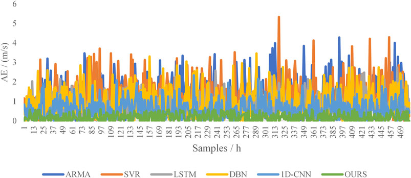
FIGURE 13. Absolute errors of the different models.

TABLE 1

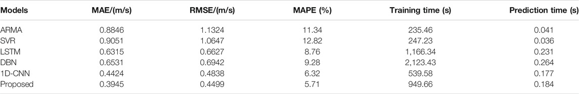
TABLE 1. Wind speed prediction results of different prediction models.

In Table 1, each error index reflects the prediction performance of the model, and the smaller the error, the better the prediction performance of the model. In the wind speed prediction of the test period, the error indexes of the proposed model are all the smallest, and the accuracy of the wind speed prediction is the highest. Compared with the ARMA, SVR, LSTM, DBN, and 1D-CNN models on MAPE, the model reduces by 5.63%, 7.11%, 3.05%, 3.57%, and 0.61%, respectively. The indicators MAE and RMSE also decrease by different ranges. In comparison with the 1D-CNN model, it can be seen that the convolutional neural network model with only the structure of 1D-CNN layer is no better than the model with the combination of 1D-CNN layer and 2D-CNN layer. As a result, the prediction error indexes of the proposed model are smaller than that of the 1D-CNN model. From the above table, we can find that the accuracy of the traditional time series-based ARMA model is not high, and only using a single wind speed as the forecasting condition is the key to its difficulty in improving its accuracy. We can also find that the prediction accuracy of the traditional machine learning model SVR is lower than that of deep learning model in tasks with a large sample size. The main reason lies in the limitations of SVR itself. SVR can usually obtain better prediction results in the small sample training than in the deep learning model, while the prediction results in the high-dimensional large sample training are inferior to deep learning model.

From the analysis of the training and testing time, the ARMA and SVR models have a faster speed in the training time, which were 235.46 and 247.23 s, respectively, to complete the training of the model. This is because these models have fewer training parameters compared with deep learning models. The deep learning model LSTM, DBN, 1D-CNN, and proposed model have more hierarchical structures and neural units, so they are accompanied by more training parameters. More training parameters will make the model more complicated and greatly increase the burden of model training. These models have more hierarchical structures and neural units, so they have a large number of training parameters to make the model more complicated and greatly increase the burden of model training. From the comparison of training and testing time of the different models, it can be seen that the proposed model has certain advantages over other traditional deep learning models. It only took 949.66 s to complete the training of the model, and it took 0.184 s to predict 480 samples forward.

To avoid the randomness of the prediction model and the contingency of the experimental results, next, we verified the proposed model on more datasets. In addition to the dataset used in this paper (Ningbo Xiangshan Dataset, referred to as NBdata), the first dataset we chose was the Eastern Wind Integration Dataset (EWIdata) (EnerNex Corporation, 2011), which consists of wind speed for 1,326 wind generation sites in the northern states of the US. EWIdata includes 6 years of wind speed-related measurements from 2007 to 2012 with 1-h intervals. Each year contains 8,760 data samples. Another dataset we chose was collected by West Texas Mesonet (texas tech national wind, 2018). The whole dataset includes data collected in 2016 from 117 weather stations, spreading out in West Texas. We can call the dataset WTdata. Each weather station contains complete data with 1-h intervals, so the size of WTdata is 1,024,920.

We have calculated the mean and standard deviation of the above three datasets, and the results are shown in Table 2. It can be seen that the distribution of data among different datasets varies greatly; the reasons behind will not be discussed here. The comparison experiments of the prediction models on the different datasets were carried out, and the average MAPE of the multiple groups of test data in the different datasets was used as the evaluation index. Comparison of average MAPE of the different prediction models on the different datasets is shown in Figure 14 and Table 3 shows the data of the comparative experimental results. From the analysis of the comparison results, the proposed model shows excellent prediction ability. In the case of the same dataset, compared with other prediction models, they all had the lowest average MAPE.

TABLE 2

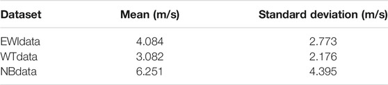
TABLE 2. The mean and standard deviation of three different datasets.

FIGURE 14

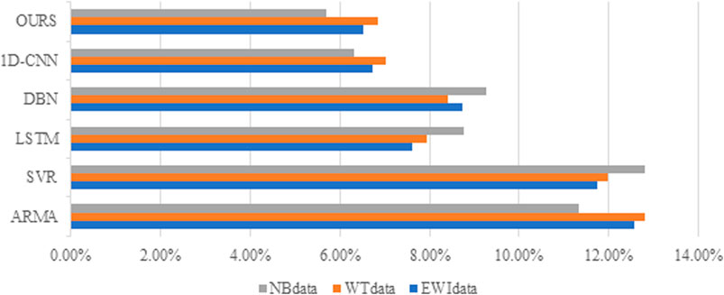
FIGURE 14. Comparison of the average mean absolute percentage error (MAPE) of the different prediction models on different datasets.

TABLE 3

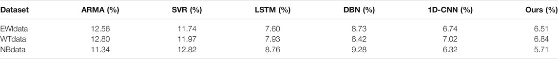
TABLE 3. Average MAPE of different prediction models on different datasets.

Conclusion

In this paper, deep convolutional neural network is applied to the prediction of wind speed in harbor anchorage, and a deep convolutional neural network model based on 1D-CNN and 2D-CNN is proposed. First, by using the model input construction method, the feature maps of the model input is constructed from the time series of each meteorological parameter, providing the model in this paper with the input data type with two-dimensional characteristics. Then, the backpropagation algorithm and Adam gradient descent algorithm were used to train the model. Finally, experimental verification was carried out in a test period of five consecutive days in randomly selected seasons. Based on the analysis of the experimental results, the following conclusions could be drawn:

1) In the proposed deep convolutional neural network model, the overfitting phenomenon easily occurs in the model after training, and the probability of this phenomenon can be reduced by L2 regularization and dropout strategy, so that the model after training can also have good predictive ability for unknown data.

2) Under the condition that the structure of the regression prediction layer does not change, the control variable method is adopted to add the CNN layer by layer to determine the structure of the deep convolutional neural network model. In the process of error analysis, it can be found that the deep convolutional neural network with 1 1D-CNN layer and 2 2D-CNN layers has the best prediction performance.

3) Compared with the traditional machine learning and deep learning models, the proposed model automatically extracts the time sequence feature information and deep abstract feature information from the input feature maps. It can effectively predict the wind speed of the harbor anchorage in the next hour, its prediction accuracy is higher than that of the traditional prediction model, and the model also has strong generalization performance on different datasets.

Data Availability Statement

The raw data supporting the conclusions of this article will be made available by the authors, without undue reservation.

Author Contributions

CH, QC, RF, and WJ contributed to the conception and design of study. CH, QC, XF, and YZ contributed to the model construction and data analysis. CH contributed to the measured data and NWP data of port anchorage collection. All authors approved the final manuscript.

Funding

This work was supported, in part, by the National Natural Science Foundation of China under Grant 41871285 and the Public Welfare Science and Technology Project of Ningbo under Grant 202002N3104.

Conflict of Interest

The authors declare that the research was conducted in the absence of any commercial or financial relationships that could be construed as a potential conflict of interest.

Publisher’s Note

All claims expressed in this article are solely those of the authors and do not necessarily represent those of their affiliated organizations, or those of the publisher, the editors, and the reviewers. Any product that may be evaluated in this article, or claim that may be made by its manufacturer, is not guaranteed or endorsed by the publisher.

References

Azad, H. B., Mekhilef, S., and Ganapathy, V. G. (2014). Long-Term Wind Speed Forecasting and General Pattern Recognition Using Neural Networks. IEEE Trans. Sustain. Energ. 5 (2), 546–553. doi:10.1109/tste.2014.2300150

CrossRef Full Text | Google Scholar

Buhan, S., Özkazanç, Y., and Çadırcı, I. (2017). Wind Pattern Recognition and Reference Wind Mast Data Correlations with NWP for Improved Wind-Electric Power Forecasts[J]. IEEE Trans. Ind. Inform. 12 (3), 991–1004. doi:10.1109/TII.2016.2543004

CrossRef Full Text | Google Scholar

Colak, I., Sagiroglu, S., and Yesilbudak, M. (2012). Data Mining and Wind Power Prediction: A Literature Review. Renew. Energ. 46 (7), 241–247. doi:10.1016/j.renene.2012.02.015

CrossRef Full Text | Google Scholar

EnerNex Corporation (2011). Eastern Wind Integration and Transmission Study. [Online]. Available at: http://www.nrel.gov/docs/fy11osti/47078.pdf (Accessed 21 Jan, 2017).

Google Scholar

Erdem, E., and Shi, J. (2011). ARMA Based Approaches for Forecasting the Tuple of Wind Speed and Direction. Appl. Energ. 88 (4), 1405–1414. doi:10.1016/j.apenergy.2010.10.031

CrossRef Full Text | Google Scholar

Huan, J., Cao, W., and Qin, Y. (2018). Prediction of Dissolved Oxygen in Aquaculture Based on EEMD and LSSVM Optimized by the Bayesian Evidence Framework. Comput. Electronics Agric. 150, 257–265. doi:10.1016/j.compag.2018.04.022

CrossRef Full Text | Google Scholar

Khodayar, M., Kaynak, O., and Khodayar, M. E. (2017). Rough Deep Neural Architecture for Short-Term Wind Speed Forecasting. IEEE Trans. Ind. Inform. (99), 1–1. doi:10.1109/TII.2017.2730846

CrossRef Full Text | Google Scholar

Khodayar, M., and Teshnehlab, M. (2016). Robust Deep Neural Network for Wind Speed Prediction[C]. 2015 4th Iranian Joint Congress on Fuzzy and Intelligent Systems (CFIS), Zahedan, Iran, September 2015. doi:10.1109/CFIS.2015.7391664

CrossRef Full Text | Google Scholar

Kingma, D., and Ba, J. (2014). Adam: A Method for Stochastic Optimization[J]. Computer Science. Available at: https://arxiv.org/abs/1412.6980.

Google Scholar

Li, Y., Chen, X., Li, C., and Tang, G (2020). A Hybrid Deep Interval Prediction Model for Wind Speed Forecasting[J]. IEEE Access 99, 1. doi:10.1109/ACCESS.2020.3047903

CrossRef Full Text | Google Scholar

Liang, S., Nguyen, L., and Jin, F. (2018). A Multi-Variable Stacked Long-Short Term Memory Network for Wind Speed Forecasting[C]. 2018 IEEE International Conference on Big Data (Big Data). Seattle, WA, USA: IEEE.

Google Scholar

Liu, H., Mi, X., and Li, Y. (2018). Smart Multi-step Deep Learning Model for Wind Speed Forecasting Based on Variational Mode Decomposition, Singular Spectrum Analysis, LSTM Network and ELM. Energ. Convers. Management 159, 54–64. doi:10.1016/j.enconman.2018.01.010

CrossRef Full Text | Google Scholar

Mahdi, K., and Wang, J. (2018). Spatio-temporal Graph Deep Neural Network for Short-Term Wind Speed Forecasting. IEEE Trans. Sustainable Energ., 1. doi:10.1109/TSTE.2018.2844102

CrossRef Full Text | Google Scholar

Shokrzadeh, S., Jafari Jozani, M., and Bibeau, E. (2017). Wind Turbine Power Curve Modeling Using Advanced Parametric and Nonparametric Methods. IEEE Trans. Sustainable Energ. 5 (4), 1262–1269. doi:10.1109/TSTE.2014.2345059

CrossRef Full Text | Google Scholar

texas tech national wind institute (2018). West texas mesonet. [Online]. Available at: http://www.mesonet.ttu.edu.

Google Scholar

Zhang, C. Y., Chen, C., Gan, M., and Chen, L. (2017). Predictive Deep Boltzmann Machine for Multiperiod Wind Speed Forecasting. IEEE Trans. Sustainable Energ. 6 (4), 1416–1425. doi:10.1109/TSTE.2015.2434387

CrossRef Full Text | Google Scholar