A Novel Shale Gas Production Prediction Model Based on Machine Learning and Its Application in Optimization of Multistage Fractured Horizontal Wells

Shale gas production prediction and horizontal well parameter optimization are significant for shale gas development. However, conventional reservoir numerical simulation requires extensive resources in terms of labor, time, and computations, and so the optimization problem still remains a challenge. Therefore, we propose, for the first time, a new gas production prediction methodology based on Gaussian Process Regression (GPR) and Convolution Neural Network (CNN) to complement the numerical simulation model and achieve rapid optimization. Specifically, through sensitivity analysis, porosity, permeability, fracture half-length, and horizontal well length were selected as influencing factors. Second, the n-factorial experimental design was applied to design the initial experiment and the dataset was constructed by combining the simulation results with the case parameters. Subsequently, the gas production model was built by GPR, CNN, and SVM based on the dataset. Finally, the optimal model was combined with the optimization algorithm to maximize the Net Present Value (NPV) and obtain the optimal fracture half-length and horizontal well length. Experimental results demonstrated the GPR model had prominent modeling capabilities compared with CNN and Support Vector Machine (SVM) and achieved the satisfactory prediction performance. The fracture half-length and well length optimized by the GPR model and reservoir numerical simulation model converged to almost the same values. Compared with the field reference case, the optimized NPV increased by US$ 7.43 million. Additionally, the time required to optimize the GPR model was 1/720 of that of numerical simulation. This work enriches the knowledge of shale gas development technology and lays the foundation for realizing the scale-benefit development for shale gas, so as to realize the integration of geological engineering.

Introduction

In recent years, the successful development of unconventional petroleum resources, especially shale gas, indicates that the oil and gas industry has made substantial breakthroughs and innovations in theory and technology, greatly expanding the field of petroleum exploration (He et al., 2020). At present, China has built hundreds of billion cubic meters of marine shale gas fields in the upper Yangtze region, such as Fuling, Changning, and Weiyuan (Jia et al., 2016). Shale gas exists in the micro nanopores of shale in the form of free adsorption, which requires horizontal wellbores and hydraulic fracture treatment to develop effectively (Chen et al., 2020; Hu et al., 2021; Yang et al., 2021). The economic benefit of many shale gas wells is often in the boundary benefit, so it is critical to balance the investment and profit. The fracture half-length and horizontal well length have a great influence on the entire investment and profit. Reservoir numerical simulation results show that revenue increases with the rise of fracture half-length, whereas the simulation results of hydraulic fracturing illustrate that the fracturing cost increases with the rise of the half-length (Figure 1). When the NPV (income minus expenditure) reaches the maximum value, the half-length is optimal. There is a similar relationship between the horizontal well length and the NPV. Therefore, it is of great significance to determine the optimal fracture half-length and horizontal well length for oil and gas field development.

FIGURE 1

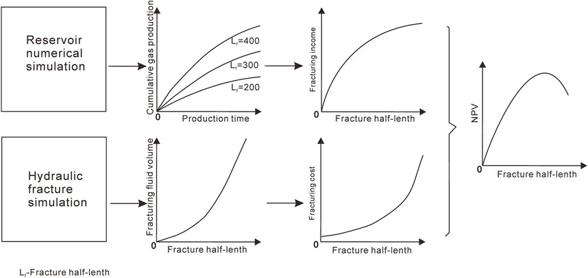
FIGURE 1. Economic optimization diagram [modified after (Li, 2009)].

There are currently two main approaches for determining optimal fracture half-length and horizontal well length. The first one is to compare several design schemes and then determine optimal fracture half-length and horizontal well length empirically, which is often used in practical production. Although this method is simple and easy to implement, it relies heavily on human experience and is difficult to get the optimal solution due to many factors of reservoir geological uncertainty. The second one is the computation optimization method based on optimization theory and reservoir numerical simulation. The main idea is to set the objective function (e.g., the NPV) and then utilize an optimization algorithm to call the numerical simulation software to obtain the optimal solution, which has been studied extensively (Babaei and Pan, 2016; Jahandideh and Jafarpour, 2016). Xu et al. (2018) combined the embedded discrete fracture model (EDFM) and intelligent algorithm to maximize the NPV. Differential evolution (DE) has been employed on a shale gas reservoir simulation model to optimize fracture half-length and fracture spacing (Rammay and Awotunde, 2016). Wang and Chen (2019a) proposed a generalized differential evolution (GDE) algorithm to optimize the well spacing, fracture spacing, half-length, and conductivity of tight oil horizontal wells. Although it has high precision and is recognized as the standard decision-making technique, it requires significant resources in terms of labor, time, and computation. Because each single well optimization needs hundreds of iterations, and each iteration takes more than 10 min, the optimization of fracture parameters in the whole area needs tens of thousands of iterations, which means more than 2 months. The traditional computation optimization is completely dependent on numerical simulation, which is inefficient and difficult to converge quickly. Therefore, we need a shale gas production forecasting model with high efficiency and good performance to optimize fracture half-length and horizontal well length.

A practical alternative is to use a proxy model, which is well suited for repeated calculations. There are two main types of surrogate models, where one is the reduced physical model (Wilson and Durlofsky, 2013; Pouladi et al., 2017), and the other one is the data-driven model (Zhou et al., 2014; Kulga et al., 2017; Wang and Chen, 2019b; Wang et al., 2021; Xue et al., 2021). The data-driven model can quickly establish a mathematical model approaching the accuracy of the numerical simulation model by sampling the reservoir numerical simulator. It is reported that GA recursive sampling assisted a dynamically updated Artificial Neural Network (ANN) method to optimize production (Golzari et al., 2015). A data-driven forecasting technique is built based on ANN to complement the simulator-based model (Kulga et al., 2017). The oil production models are developed based on Random Forests (RFs), Support Vector Regression (SVR), and Gradient-Boosting Machine (GBM) (Schuetter et al., 2018). However, few researchers have optimized hydraulic fracture parameters assisting the data-driven model. Consequently, in this study, we propose adopting the Gaussian Process Regression (GPR) and Convolution Neural Network (CNN) in the machine learning field as the proxy models to predict production and utilize the GA and penalty function method to obtain the optimal solution based on these two proxy models.

GPR is a supervised learning model based on Bayesian theory, which has a strict statistical learning foundation and can solve the complex regression problems (Yu et al., 2017). Compared with other regression methods, GPR is characterized by high prediction accuracy, strong generality, and robust performance, which has been widely used in the machine learning field (Ganti and Khare, 2020; Zhang and Xu, 2020). As a new research direction in machine learning, deep learning has attracted growing attentions (Zheng et al., 2020). CNN is a kind of multilayer feedforward neural network with convolution operations. Unlike the BP, which only has a fully connected layer, the local connection, weight sharing, and pooling operation of CNN can enhance the representation ability and robustness of a network (Karpathy et al., 2014).

This research attempts to build a robust and rapid production prediction proxy model based on machine learning to complement the physical-driven model and obtain the optimal fracture parameters by applying the optimization algorithm on the proxy models. The article has been organized in the following way. Specifically, the sensitivity analysis of reservoir parameters and hydraulic fracturing parameters is carried out to study the contribution of each parameter to production. The n-factorial experimental design is used to design the initial experiments, and 256 cases are obtained. Then 256 cases are simulated by CMG, and the dataset is constructed by combining the simulation results with the case parameters. Subsequently, the gas production model is built by GPR, CNN, and SVM based on the dataset. Finally, the optimal model of the three models is combined with the optimization algorithm to maximize the NPV and obtain the optimal fracture half-length and horizontal well length. The performance of the proxy model is assessed in terms of time efficiency and prediction accuracy by comparing the results with the simulator-based approach.

Data Preparation

Before establishing the data-driven model, it is necessary to collect the data of production and geological engineering parameters. It is better to collect real data, but if there is no high quality real data, numerical simulation data can be used. In this study, a numerical simulator is applied to obtain annual production data of shale gas under the given geological engineering parameters. At present, about 30 wells have been drilled in this area. The shale is mainly developed in the Lower Silurian Longmaxi Formation to the Upper Ordovician Wufeng Formation, with an effective thickness of 30–40 m. The buried depth of the gas reservoir is 2000–3000 m, the pressure coefficient is 1.1–1.3, and the formation temperature is about 80°C. The average matrix porosity, average matrix permeability, average matrix gas saturation, and the average adsorbed gas content are 4%, 0.00003 md, 65%, and 3 m³/t, respectively.

According to the reservoir geological parameters and horizontal well engineering parameters in the study area, a single-well numerical model of shale gas multistage fracturing horizontal well was established by CMG software (Table 1).

TABLE 1

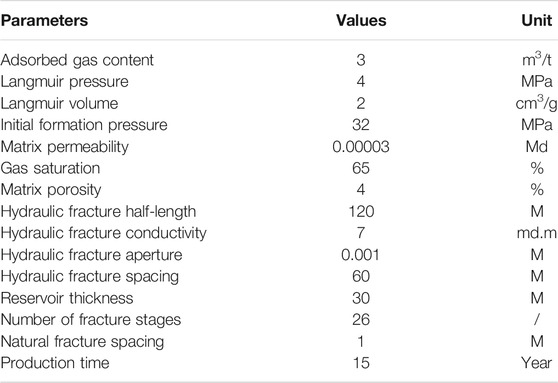
TABLE 1. Basic parameters of shale gas numerical model.

The gas reservoir size was 4200 m $\times$ 500 m $\times$ 30 m, and the reservoir type was the dual-porosity and dual-permeability model. The established reservoir model was a rectangular grid system with horizontal wells in the center of the model. The horizontal well was placed in the middle layer in the reservoir model, and the production duration was set to 15 years. The hydraulic fracture propagated along the direction of the maximum principal stress. Figure 2 shows a top view of the hydraulic fracture model. The grid we set was 20 m. Local grid refinement (LGR) was applied to simulate fluid flow in hydraulic fractures accurately.

FIGURE 2

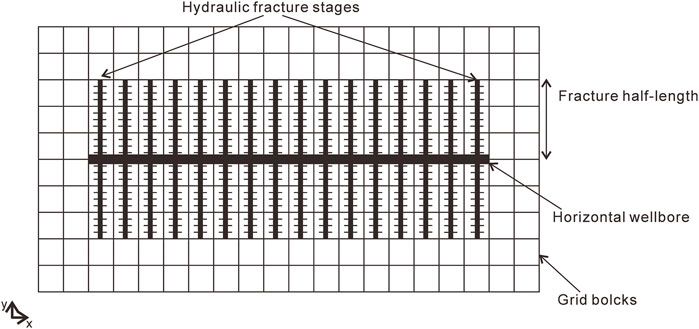
FIGURE 2. Top view of the numerical simulation model.

By analyzing the study area’s geological engineering conditions, we selected four key influencing parameters, including matrix porosity, matrix permeability, fracture half-length, and horizontal well length. The n-factorial experimental design procedure was utilized to build a data set for building the proxy model. The range of four factors were divided into four equally-spaced levels (Table 2), so 256 cases were obtained. Other experimental design method, such as response surface design, only needs 29 experiments, which cannot achieve the required accuracy. Therefore, an n-factorial experimental design was adopted. If the variables increase, we can use Latin hypercube design, response surface design, and so on. All cases were run using CMG-GEM numerical simulation software to obtain the corresponding performance (Supplementary Table S1).

TABLE 2

TABLE 2. The levels of four factors.

Methods

Gaussian Process Regression Model

Principle of GPR

In recent years, machine learning has been widely used in all walks of life. The purpose of machine learning is to use algorithms to build statistical models for the collected data and to solve practical problems by building good statistical models. There are many regression learning algorithms: nonlinear regression, Support Vector Machine regression (SVM), Gaussian Process Regression (GPR), Regression Tree (RT), Random Forest (RF), and so on. Considering the advantages of GPR model mentioned above, we use GPR model (Hamdi et al., 2017) to build production prediction model.

GPR is a nonparametric probability model for regression analysis of data based on the Bayesian principle. The basic principle of GPR is as follows. Firstly, given the Gaussian Process (GP) prior distribution, the mean and covariance of the GP posterior distribution are calculated based on the prior and the hypothesis of training data (joint Gaussian distribution). When the input data ($x_i$) and the output data ($y_i$) of the training data are given, the trained GPR model can predict the new output data ($y^{\ast }$) according to input data ($x^{\ast }$).

Assuming that the noise between the observed value and the prediction function satisfies the normal distribution, the expressions are as follows (Zhang et al., 2020):

$y_i=f\left(x_i\right)+\epsilon (1)$

$\epsilon \sim N(0,{\sigma }^2)(2)$

where $x_i$ is the input vector, $f$ is the prediction function, and$y_i$is the observation value polluted by noise. $\epsilon$ is noise, following the normal distribution ($N$) of mean value 0 and variance ${\sigma }^2$.

GP is a set of any finite number of random variables with a joint Gaussian distribution, whose properties are entirely determined by the mean function and the covariance function:

$f\left(x\right)\sim GP(m\left(x\right),k(x,x\prime ))(3)$

$m\left(x\right)=E\left[\left(f\left(x\right)\right)\right](4)$

$k\left(x,x^{\prime }\right)=E\left[\left(f\left(x\right)-m\left(x\right)\right)\left(f\left(x^{\prime }\right)-m\left(x^{\prime }\right)\right)\right](5)$

where $m\left(x\right)$ and $k\left(x,x^{\prime }\right)$ are the mean function and covariance function, respectively. The prior distributions of the observed values $y$ are as follows:

$y\sim N[u,K\left(x,x\right)+{\delta }_n^{2}I](6)$

According to Bayes principle, the prior joint distribution of the observed value $y$ and the predicted value $f_{\ast }$ (the output value corresponding to $x_{\ast }$) are

$\left[\begin{array}{c}y\\ f_{\ast }\end{array}\right]\sim N\left(0,\left[\begin{array}{cc}K\left(X,X\right)+{\delta }_n^2{I}_n& K(X,x_{\ast })\\ K(x_{\ast },X)& k(x_{\ast },x_{\ast })\end{array}\right]\right),(7)$

where $K\left(X,X\right)=K_n=\left(k_{ij}\right)$ is the symmetric positive definite matrices of order $\text{n}\times \text{n}$, the matrix element $\left(k_{ij}\right)=k(x_i,x_j)$ is implemented to measure the correlation between $x_i$ and $x_j$, and $K\left(X,x_{\ast }\right)=K{(x_{\ast },X)}^T$ are the $\text{n}\times 1$ covariance matrix between the test input values $x_{\ast }$ and the training input values. $K\left(x_{\ast },x_{\ast }\right)$ is covariance matrix of test input values $x_{\ast }$. $I_n$ is an n-dimensional identity matrix.

According to the marginal distribution property of normal joint distribution, the posterior distribution of $f_{\ast }$ can be modeled as

$f_{\ast }|X,y,x_{\ast }\sim N\left(\overline{f_{\ast }},cov\left(f_{\ast }\right)\right) (8)$

$\overline{f_{\ast }}=K\left(x_{\ast },X\right){[K\left(X,X\right)+{\sigma }_n^2{I}_n]}^{-1}y (9)$

$\text{cov}\left({\text{f}}_{\ast }\right)=k\left(x_{\ast },x_{\ast }\right)-K\left(x_{\ast },X\right)\times K\left(X,X\right)+{\sigma }_n^2{I}_n{]}^{-1}K\left(X,x_{\ast }\right),(10)$

where $\overline{f_{\ast }}$ and $cov\left(f_{\ast }\right)$ are the mean and variance of the predicted value $f_{\ast }$.

Covariance Functions Optimization

Since the covariance function in the GPR method is a symmetric function satisfying the Mercer condition, the covariance function is equivalent to a kernel function, which can be parameterized by vectors $\theta$ in kernel parameters. Therefore, the expression of a covariance function is $\text{k}(x_i,x_j|\theta )$. Kernel functions can be divided into two types according to the characteristic length scale. If the length scale is the same, the kernel function encompasses squared exponential kernel, exponential kernel, Matern 3/2, Matern 5/2, and rational quadratic kernel. The kernel functions with a separate length scale realizing the automatic correlation determination include ARD squared exponential kernel, ARD exponential kernel, ARD Matern 3/2, ARD Matern 5/2, and ARD Rational Quadratic Kernel. The squared exponential kernel is the most commonly used kernel function, which is defined as

$\text{k}\left(x_i,x_j\text{|}\theta \right)={\sigma }_f^2\text{exp}\left[-\frac{1}{2}\frac{{\left(x_i-x_j\right)}^T(x_i-x_j)}{{\sigma }_l^2}\right](11)$

where $x_i$ and $x_j$ are the training input data and ${\sigma }_f$ and ${\sigma }_l$ are the hyperparameters of the kernel function, which represent signal standard deviation and length scale.

Kernel function directly affect the accuracy of the GPR algorithm. We need to optimize the kernel function. The commonly used effective method for the limited dataset is cross-validation, which comprises k-fold cross-validation and leave-one-out cross-validation. K-fold cross-validation randomly divides the sample data into k copies, each time selects k-1 as the training set and the remaining one as the test set. Leave-one-out cross-validation is a special case of k-fold cross validation, where k is equal to the number of samples. This method is suitable for the case of small data.

We applied MATLAB software to establish the GPR technique to forecast production. In order to ensure the reliability of the model, the scheme of 10-fold cross-validation was adopted. The performance was evaluated using the coefficient of determination (R²) and root mean square error (RMSE).

$R^2=\frac{{{\displaystyle \sum }}_{i=1}^N[\left(z_i-z_l\right)-\left(y_i-y_l\right)]}{\sqrt{{{\displaystyle \sum }}_{i=1}^N{(z_i-z_l)}^2{{\displaystyle \sum }}_{i=1}^N{(y_i-y_l)}^2}}(12)$

$\text{RMSE}=\sqrt{\frac{1}{N}{\displaystyle \sum }_{i=1}^N{(z_i-y_i)}^2}(13)$

where $z_i$ is the gas production predicted by the data-driven model, $y_i$represents the gas production calculated by a numerical simulation model, $z_l$ represents the average gas production predicted by the data-driven model, $y_l$represents the average gas production calculated by a numerical simulation model, and $\text{N}$ is the number of samples.

Convolution Neural Network

Deep learning can achieve complex function approximation by learning a group of kernel parameters of a nonlinear network, which shows a strong ability to learn the essential characteristics from a small sample set. CNN is a multilayer feedforward neural network with a convolution structure and becomes one of the most concerned research hotspots (Wang et al., 2019; Zheng et al., 2020). Unlike the traditional fully connected feedforward neural network, CNN has the characteristics of local connection and parameter sharing, which reduces the complexity of the network and improves computational efficiency. In image processing, 2D convolution is usually used to extract features layer by layer and then complete the corresponding visual tasks. The convolution kernel size is usually square $\text{N}\times \text{N}$, and $\text{N}$ represents the width or height of the convolution kernel. In addition, convolution neural network has 1D convolution operation, which can process sequence data. The convolution kernel used is $\text{N}$, and $\text{N}$ represents the length of the convolution kernel. Similar to 2D convolution neural network, 1D convolution kernel also processes input data layer by layer to extract discriminative features, so as to complete classification, regression, and other tasks. As shown in Figure 3, the typical CNN mainly comprises the input layer, convolution layer, downsampling layer (pooling layer), full connection layer, and output layer. The convolution layer and pooling layer are the special network structure of CNN. The convolution layer is responsible for extracting the convolution features of the input data, and the pooling layer is used to down sample the convolution features to improve the robustness.

FIGURE 3

FIGURE 3. Typical structure of convolution neural network (Wang et al., 2019).

The role of the convolutional layer is to use convolution operations to extract features. The more the convolutional layers are, the stronger the expressive ability of features is. By designing multiple convolution kernels in the convolution layer, CNN can extract a variety of different types of local features and then extract higher-level features layer by layer. Finally, global features can be abstracted through deep learning of local features. A layer of CNN can contain several convolution filters (each containing a deviation coefficient). The filters in the upper left corner slide through each input image from left to right and from top to bottom, and convolution are performed in each iteration. Then, the sum of convolution result and deviation value is converted nonlinearly. Commonly used activation functions include ReLU, sigmoid, and tanh.

According to the local connection principle of CNN, each pooling layer is also composed of multiple sampling neurons, and each unit is also connected to the corresponding receptive field of the previous layer of network. But different from the convolutional layer, all the weights of the neurons in this layer and the local connection of the previous layer are fixed constants. Downsampling is performed by taking the local maximum value or the average value to generate all the local features in the same filter. The pooling operation not only further reduces the network scale and suppresses possible over-fitting, but also improves the robustness of the extracted features, while retaining the salient features and shift invariance.

The CNN proposed in this study mainly had five layers. The first layer was porosity, matrix permeability, fracture half-length, and horizontal well length, respectively. The second, third, and fourth layers were the convolutional layers, which had 5, 10, and 15 convolution kernels with a size of 3 × 1. The fifth layer was a fully connected layer with a total of 15 neurons. The output layer was the predicted gas production value. A stochastic gradient descent algorithm was used to train CNN, and the activation function was Sigmoid. The number of iterations was 5,000, and the weight values were updated repeatedly until the error meets the requirements.

1) First, input data were normalized to make all the data on the same magnitude.

${\overline{x}}_{attr}=\frac{1}{N}{\displaystyle \sum }_{i=1}^N{x}_{i,attr}(14)$

${\text{s}}_{attr}=\sqrt{\frac{1}{N-1}{\displaystyle \sum }_{i=1}^N{\left(x_{i,attr}-{\overline{x}}_{attr}\right)}^2}(15)$

${\widehat{X}}_{i,attr}=\frac{x_{i,attr}-{\overline{x }}_{attr}}{s_{attr}},(16)$

where $attr$ denotes porosity, matrix permeability, fracture half-length, and well length, ${\overline{x}}_{attr}$ is the average $attr$ value of all samples, $x_{i,attr}$ donates the value of the i-th sample, $s_{attr}$is the variance of $attr$ of all samples and ${\widehat{X}}_{i,attr}$ is the normalized value of the sample, and N is the number of samples.

2) Three convolution layers with a different number of kernels performed 1D convolution on the input data:

$Y_1^{CNN}=ReLU\left(W_1\mathrm{ʘ}X+b_1\right)(17)$

$Y_2^{CNN}=ReLU\left(W_2\mathrm{ʘ}{Y}_1^{CNN}+b_2\right)(18)$

$Y_3^{CNN}=ReLU\left(W_3\mathrm{ʘ}{Y}_2^{\mathit{C}NN}+b_3\right)(19)$

where $Y_1^{CNN}$, $Y_2^{CNN}$, and $Y_3^{CNN}$ are the outputs of the second, third, and fourth layers, and $\text{ReLU}$ is the activation function. $W_1\in R^{5\times 1\times 2}, W_2\in R^{10\times 5\times 2}\text{,and} W_3\in R^{15\times 10\times 2}$ are parameters of the convolution kernels of the second, third, and fourth layers, respectively. $b_{1, } b_{2, }{b}_3$ are the bias. The symbol $ʘ$ denotes the convolution operation.

3) Next, the fully connected layer was utilized to predict the gas production.

$Q_{gas}=\text{Relu}(W_4\times Y_3^{CNN}+b_4),(20)$

where $Q_{gas}$ is cumulative gas production in 15 years. Averpool denotes the average pooling layer, $W_4\in R^{15\times 1}$ denotes the parameters of the fully connected layer, $b_4$is the bias.

4) Finally, the performance was evaluated using R² and RMSE.

Support Vector Machine Regression

SVM is based on the theory of small sample statistical learning proposed by Vapnik (2000), which focuses on the statistical learning rule under small sample data. Compared with neural network, SVM has strict theoretical and mathematical foundation and has strong generalization ability. It also has a weak dependence on the number of samples. The basic idea of support vector machine regression theory is to find a nonlinear mapping ($\varphi$) from input space to output space. Through this nonlinear mapping, the data ($\text{x}$) are mapped to a high-dimensional feature space ($\text{F}$). The nonlinear regression function of SVM is as follows:

$\text{f}\left(\text{x}\right)={\displaystyle \sum }_{i=1}^n\left(a_i-a_i^{\ast }\right)K\left(x_i,x_j\right)+b(21)$

where $a_i$ and $a_i^{\ast }$ are Lagrange multiplier and $K\left(x_i,x_j\right)$ is kernel function.

The kernel function of the SVM converts nonlinear separable samples into a linearly separable feature space. Different kernel functions produce different classification hyperplanes, so the kernel function has a direct impact on the performance of SVM. We applied MATLAB software to establish the SVM technique to forecast production. In order to ensure the reliability of the model, the scheme of 10-fold cross-validation was adopted. The performance of different kernel functions was evaluated using the R² and RMSE.

Economic Model

To improve the economic benefit of the study area, the economic NPV is considered the objective function to optimize the fracturing parameters of shale gas horizontal wells.

NPV consists of two parts: cash inflow and cash outflow. According to the data of the study area, we adopt the following NPV mathematical model:

$\text{NPV}(x_f,\text{L})={\displaystyle \sum }_{n=1}^{N_t}\left[\frac{1}{{(1+b)}^t}(P_0{Q}_{gas}(x_f,\text{L})-C_{operating}-C_{tax})\right]-(C_{ground}+C_{well}\left(\text{L}\right)+C_{fracture}(x_f,\text{L})),(22)$

where $t$ is time, (year); $\text{b}$ is discount rate, (%);$P_0$ is the gas price, (USD/m³); $Q_{gas}$ is annual gas production, (m³/year); $C_{operating}$ is annual operating cost, (USD/year); $C_{tax}$ is tax, (USD/m³); $C_{ground}$ is ground cost, (USD); $C_{well}$ is drilling cost, (USD); $C_{fracture}$ is fracturing cost, (USD);$\text{ L}$ is horizontal well length, (m); $x_f$ is fracture half-length, (m). L and $x_f$ are optimization variables. In the optimization process, the ranges of the two variables are 50–200 m, 1,000–4,000 m, respectively. Related parameters are shown in Table 3.

TABLE 3

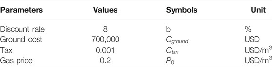
TABLE 3. Parameters for NPV calculation.

In the process of hydraulic fracturing, tens of thousands of cubic meters of fracturing fluid and thousands of tons of proppant are pumped into the ground to produce fractures and release natural gas. Therefore, fracturing cost mainly includes the cost of pumping fracturing fluid and proppant. A larger number of researches have been conducted on the relationship between the volume of fracturing fluid and fracture half-length (Rammay and Awotunde, 2016; Yang et al., 2017; Wang and Chen, 2019). Here, the relationship between them is obtained by referring to Rammay and Awotunde (2016) and Nordgren (1970).

$x_f=\frac{Q\left(\text{W}+2S_P\right)}{4\pi \text{h}{C}^2}({\text{e}}^{x^2}\text{erfc}\left(x\right)+\frac{2x}{\sqrt{\pi }}-1)(23)$

$\text{W}=\left(\frac{64}{3\pi }(n^{\prime }+1)\right){ }^{\frac{1}{2(n^{\prime }+1))}}\left(\frac{6q}{\text{H}}\right){ }^{\frac{n^{\prime }}{2(n^{\prime }+1))}}\left(\frac{K_{\alpha }(1-\text{vH}L)}{G}\right){ }^{\frac{1}{2(n^{\prime }+1)}}(24)$

$x=\frac{2C\sqrt{\pi t}}{W}(25)$

$K_{\alpha }=k^{\prime }{\left(\frac{2n^{\prime }+1}{3n^{\prime }}\right)}^{n^{\prime }}(26)$

${\text{e}}^{x^2}\text{erfc}\left(x\right)=0.254829592y-0.284496736y^2+1.42143741y^3-1.453152027y^4+1.06140429y^5(27)$

$\text{y}=\frac{1}{1+0.3275911x}(28)$

$\text{V}=\text{Qt},(29)$

where $x_f$ is fracture half-length, (m); $Q$ is displacement, (m³/min); $W$ is fracture width (m); $S_p$ is spurt loss volume, (m³/m²); $\text{h}$ is fracture height, (m); $C$ is fluid loss coefficient, (m/$\sqrt{min}$), $n^{\prime }$ is rheological index, $k^{\prime }$ is the consistency coefficient, (MPa·s); $G$ is shear modulus, (MPa); $\text{v}$ is Poisson’s ratio; $t$ is time, (min); $\text{erfc}\left(x\right)$ is error compensation function of $x$; V is amount of fracturing fluid per stage (m³/stage). Table 4 shows the input parameters for calculating the fracture half-length according to the amount of fracturing fluid.

TABLE 4

TABLE 4. The input parameters for calculating the fracture half-length.

By analyzing the fracturing cost of horizontal wells in the study area, the relationship between fracturing fluid volume and fracturing cost is established, so as to finally obtain the relationship between fracture half-length and fracturing cost.

$C_{fracture}=\left((1.9402T+1.0506Q_{transport}/10000+0.039117VL+0.14425PL+0.25155L+0.25155L+Q_{tubing}+310.3908)10000\right)/6.5;(30)$

$\text{T}=26.83+0.00974L+(0.012987VL-27.214\text{L})/23040(31)$

$Q_{tubing}=(183.4585+(0.012987L-137.363)/6.5(32)$

$Q_{transport}=(12648.08+17.574\text{L}),(33)$

where $C_{fracture}$ is fracturing cost, (USD); T is construction time, (day); L is horizontal well length, (m); $Q_{transport}$ is transportation cost, (USD); $Q_{tubing}$ is tubing costs, (USD); $P$ is the volume of proppant. The volume ratio of proppant to fracturing fluid is 0.035.

The drilling cost is related to the length of the horizontal section. By analyzing the drilling cost data in the study area, the relationship between the length of the horizontal section and the drilling cost can be obtained.

$C_{well}=\left(9060544+1137.55\left(3500+L\right)+\left(2.5985\left(3500+L\right)+104211\right)\left(9.1+0.0000028531L^2+0.0036156L+50.09\right)+149.116L+44160 exp\left(0.0002\left(3500+L\right)\right)+33514exp\left(0.0006\left(L+700\right)\right)+26458exp\left(0.00039\left(L+700\right)\right)\right)(34)$

The formula of operating cost is as follows:

$C_{operating}=\mathrm{37,000}+0.05Q_{gas}(35)$

Optimization Algorithm

Optimization algorithms are divided into traditional gradient-based optimization algorithms and evolutionary algorithms. Traditional gradient-based optimization algorithms, such as the penalty function method and the conjugate gradient method, have fast convergence speed, but they are easy to fall into the local optimum. Evolutionary algorithms such as particle swarm optimization (PSO) algorithm (Li et al., 2012) and genetic algorithm (GA) (Cen et al., 2016) have good global search capabilities, but their convergence speed is relatively slow. In practical application, we can employ these two optimization algorithms to benefit each other. In this article, we used MATLAB to build GA model and penalty function method.

Genetic Algorithm

As a classical global optimization algorithm, GA has been widely used in many fields, such as industrial design and economic management (Golzari et al., 2015; Zhang et al., 2019). GA starts the search process from a set of initial solutions, called population. Each individual in the population is a solution to the problem, called a chromosome. These chromosomes continue to evolve in subsequent iterations, known as heredity. GA is mainly realized by crossover, mutation, and selection. The next generation of chromosomes generated by crossover or mutation operations is called offspring. The quality of chromosomes is measured by fitness. According to the fitness, a certain number of individuals are selected from the previous generation and offspring as the next generation population and then continue to evolve. After several generations, the algorithm converges to the best chromosome, which is likely to be the optimal solution.

Penalty Function Method

The basic idea of the penalty function method is to transform the constraint into a kind of penalty function and add it to the objective function, thus transforming the constrained optimization problem into a series of unconstrained optimization problems (Hao et al., 2021). The penalty function method includes the interior point method, external penalty function method, and multiplier method. This research mainly adopts the interior point method, which has the advantages of simple structure and strong adaptability.

Optimization problems with general constraints are

$\text{min }f\left(x\right) x\in R^n(36)$

$\text{Subject}\text{to}{c}_{i }\left(x\right)>0, i=1,\dots ,m(37)$

$D_0=\left\{x\in R^n\text{|}{c}_{i }\left(x\right)>0, i=1,\dots ,m\right\} \ne \varnothing (38)$

where $f\left(x\right)$ is the objective function, $c_{i }\left(x\right)$ is the constraint condition, and $D_0$ is the feasible region. The interior point method needs to construct the following augmented objective functions:

$\text{p}\left(\text{x},\text{σ}\right)=\text{f}\left(\text{x}\right)+\text{σ}\overline{p}\left(\text{x}\right)(39)$

where$\text{ σ}>0$ is penalty parameter and $\overline{p}\left(\text{x}\right)$ is obstacle function. It needs to satisfy the following properties: when $\text{x}$ tends to the boundary at $D_0$, at least one $c_{i }\left(x\right)$ tends to 0 and $\overline{p}\left(\text{x}\right)$ tends to infinity. There are two forms of obstacle function:

$\overline{p}\left(\text{x},\text{σ}\right)=-{\displaystyle \sum }_{i=1}^m\text{ln}\left[c_i\left(x\right)\right](40)$

$\overline{p}\left(\text{x},\text{σ}\right)=-{\displaystyle \sum }_{i=1}^m\frac{1}{c_i\left(x\right)}(41)$

In this way, when $\text{x}$ is in $D_0$, it is finite; when $\text{x}$ is close to the boundary, $\overline{p}\left(\text{x}\right)\to +\infty$ the value of the augmented objective function tends to infinity, so it is severely punished.

Since the minimum point of constrained optimization problem is generally reached at the boundary of feasible region, the penalty factor in interior point method requires ${\sigma }_k\to 0$, so the solution problem is transformed into solving nonsequence constrained optimization subproblem.

$\min \text{p}\left(\text{x},\text{σ}\right)=f\left(x\right)+{\sigma }_k\overline{p}\left(\text{x}\right)(42)$

The overall optimization framework is shown in Figure 4.

FIGURE 4

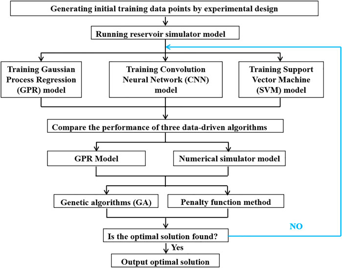
FIGURE 4. Flowchart of the optimization algorithm.

Result and Discussion

Sensitivity Analysis

Matrix porosity, matrix permeability, horizontal well length, and fracture half-length have an influence on gas production. In order to intuitively study the influence of various factors on the cumulative gas production, we made a correlation diagram. Matrix porosity and horizontal section length have linear relationships with gas production, while matrix permeability and fracture half-length are logarithmically related to the gas production (Figure 5). The results of the sensitivity analysis show that these four factors have a significant influence on gas production.

FIGURE 5

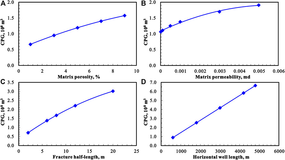
FIGURE 5. (A) The relationship between matrix porosity and CGP (Cumulative gas production of 15 years). (B) The relationship between matrix permeability and CGP. (C) The relationship between fracture half-length and CGP. (D) The relationship between horizontal well length and CGP.

Comparison of Gas Prediction Models

GPR model is parameterized by kernel function, which directly affects the prediction accuracy. In order to obtain a suitable kernel function, we experimented with the ten kernel functions. Through comparing different kernel functions (Table 5), we found that ARD squared exponential outperformed other kernel functions by providing higher R² and lower RMSE, so we chose it as the final kernel function.

TABLE 5

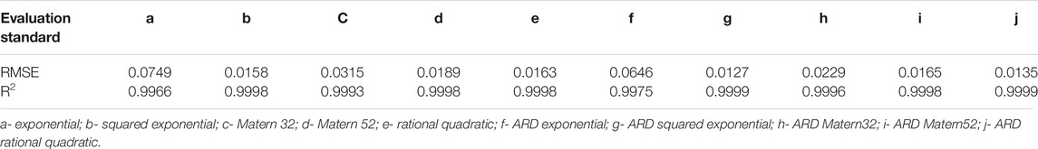
TABLE 5. Comparison of kernel function precision.

Different kernel functions will affect the prediction accuracy of SVM. As can be seen from Table 6, the polynomial kernel function provides higher R² and lower RMSE, so we chose it as the final kernel function. According to the optimal kernel function and kernel parameters of SVM, we can accurately establish the production prediction model.

TABLE 6

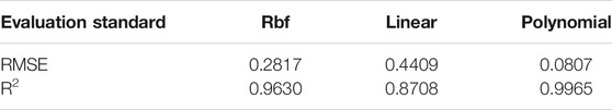
TABLE 6. Comparison of kernel function precision.

In this section, the performances of the GPR model, CNN model, SVM model and model are compared. 256 experiments (Table 2) were acquired from the initial experimental design for the shale gas estimation model. The cross-validation and kernel function optimization were utilized to improve the prediction accuracy. R² and RMSE were used to compare the performance of three models on the validation set. As shown in Figure 6, R² of GPR, CNN, and SVM is 99.99, 98.07, 99.65, and 99.6%, respectively, and RMSE is 0.0127, 0.1690, and 0.0807, respectively. The GPR model reveals competitive modeling capabilities compared with CNN and SVM. This gives confidence in the model’s predictive ability. Therefore, the GPR model is more reliable. The proxy model constructs an approximate model of production prediction by collecting a small number of samples. It is applied when calculating the production instead of directly calling the reservoir numerical simulation program, which effectively improves the optimization speed.

FIGURE 6

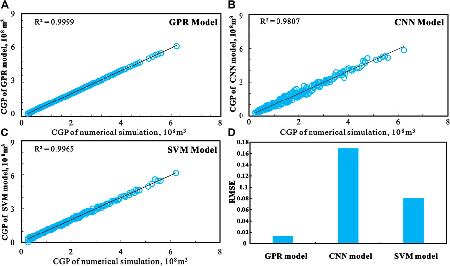
FIGURE 6. (A) Comparison of production predicted by the GPR model and numerical simulation model. (B) Comparison of production predicted by the CNN model and numerical simulation model. (C) Comparison of production predicted by the SVM model and numerical simulation model. (D) RMSE of GPR model, CNN model and SVM model.

Additionally, to further study the performance of GPRR model to predict the gas production per year, we calculated the gas production of each year for 15 years under a given geological engineering parameter using surrogate model and compared it with the results obtained by a simulator-based approach. The fixed parameters are porosity, permeability, fracture half-length, and horizontal section length of 4%, 0.00003 md, 120 m, and 1,600 m respectively.

It is observed that the two production decline curves are relatively close, indicating that the GPR model is capable of estimating well performance (Figure 7). Therefore, the GPR model has high reliability. Besides, the GPR approach is faster than the numerical simulation technique. The numerical model takes about 10 min to complete each simulation on the machine with I7-6700 3.4 GHz CPU, while the data-driven model can calculate the output within a minute. Therefore, the GPR model is a good alternative to numerical models.

FIGURE 7

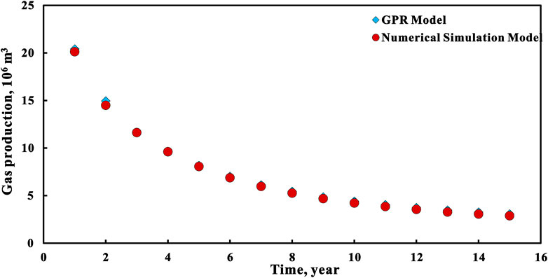
FIGURE 7. Comparison of production decline curves between GPR model and numerical simulation model.

Comparison of Optimization Results

An important application of production prediction model is to optimize fracturing design and horizontal well parameters. Therefore, in order to verify the effectiveness of the established production proxy model, we used GA and penalty function to optimize the fracture half-length and horizontal segment length based on GPR model and NPV model established in Methods. Because porosity and permeability were not involved in the optimization, the porosity and permeability were fixed at 4% and 0.00003 md, respectively. At the same time, the fracture half-length and horizontal section length are optimized based on the numerical simulation model. We used the optimization algorithm to iterate for 100 times and obtained the following results.

The initial fracture half-length, horizontal well length, and NPV of field reference case are 100 m, 1,600 m, US$ -1.13 million, respectively. The fracture half-length, horizontal well length, and NPV optimized by GA based on GPR model and numerical simulation model converge to almost the same values (Table 7). Compared with the field reference case, the optimized NPV increased by US$ 7.43 million. Therefore, according to the optimization results, the GPR model coupled with GA and penalty function method can meet the requirements of reservoir well layout optimization. We also noticed that the optimization time of GPR model is 1/720 of that of the numerical simulation model, which dramatically improves the optimization efficiency (Table 7). This proves the applicability and strength of the GPR model.

TABLE 7

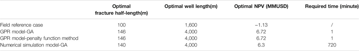
TABLE 7. Optimization results.

It is noted that the optimized horizontal well length reaches the maximum values (4000 m). Since drilling cost is a function of measuring depth and horizontal well length, there is an incentive to increase reservoir contact by extending the horizontal section to recover the cost of drilling vertical section. In addition, longer horizontal wells have created more room for hydraulic fracture treatments, and, thus, increasing shale gas production. This result is consistent with the industry trend toward a longer horizontal well (Wilson and Durlofsky, 2013). Meanwhile, it is worthwhile to point out that the optimized fracture half-length is not the maximum value in the range. This can be attributed to the fact that the rate of revenue increase is not as fast as the cost increase rate.

To prove the adaptability of the GPR model in the variable economic conditions, changes in natural gas prices are considered. The gas price ranges from 0.138 USD/m³ to 0.261 USD/m³. Figure 8 displays the relationship between natural gas price and optimal fracture parameters. As the price of natural gas increases, the optimal fracture half-length gradually increases, but the optimal horizontal well length remains unchanged. The increase of optimal fracture half-length could be attributed to the increase in income exceeding the increase in expenditure. With a higher gas price, it is reasonable to use a longer horizontal well length and longer fracture half-length.

FIGURE 8

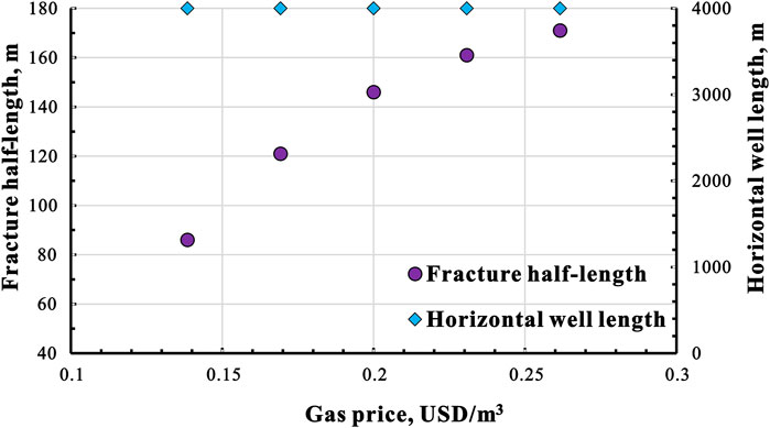
FIGURE 8. Relationship between optimal fracture half-length, horizontal well length, and gas price.

The benefits of data-driven models are evident when a large number of numerical simulations are needed without enough time and computing resources. This fast proxy model can optimize the engineering parameters of a single well in a minute, and its accuracy is almost equal to that of the numerical model that takes 12 h. If there are more wells, it takes dozens or even hundreds of days to run reservoir simulation, resulting in an unaffordable computational cost. The efficiency and flexibility of the proxy model enable engineers to estimate gas production and optimize fracture parameter accurately.

Although the data-driven model possesses many advantages, the potential limitations should not be ignored. The accuracy of the numerical simulation model limits the prediction accuracy of the surrogate model. It should be noted that the aim of GPR model is not to replace the numerical simulation model but to perform fast and efficient modeling. The optimized fracture half-length is constrained by fixed fracture spacing and fracture conductivity. The fracture spacing and fracture conductivity should be incorporated in the optimization process in the future. Complex fracture networks and geomechanical properties are not considered in this work. In future work, the geomechanical properties will be integrated into the rapid and robust model for shale gas production.

Conclusion

In this article, data-driven prediction techniques, including GPR, CNN, and SVM models, were developed and verified by combining machine learning with a reservoir numerical program. Following that, the GPR model and reservoir simulator were driven by the evolutionary algorithm and traditional optimization algorithm. The main conclusions are summarized as follows:

1) The developed GPR model outperforms the CNN and SVM models by providing higher R² and lower RMSE, indicating it can quickly establish a mathematical model approaching the accuracy of the numerical simulation model by sampling the numerical model.

2) The optimal half-length, horizontal well length, and NPV obtained by the GPR model and simulator-based model converge to almost the same value, further verifying the GPR model’s reliability. Whereas the GPR model’s optimization time is only 1/720 of that of the numerical simulation model, which dramatically improves the optimization efficiency. Compared with the field reference case, the optimized NPV increased by US$ 7.43 million.

3) The developed data-driven model based on the optimization methodology provides a substantially fast and accurate substitute for the numerical-simulation-assisted optimization algorithm. These findings provide a basis for the rapid optimization of the whole region. In the future, more parameters such as fracture spacing and fracture conductivity will be considered in the optimization process.

Data Availability Statement

The original contributions presented in the study are included in the article/Supplementary Materials; further inquiries can be directed to the corresponding authors.

Author Contributions

HW, SL, and TH designed the research. HW wrote the manuscript. FC discussed the results. XH and JZ performed data analyses. ZF prepared the figures and tables.

Funding

This work was supported by the National Major Science and Technology Project (2016ZX05061) and research project funded by SINOPEC (P19017-3).

Conflict of Interest

Authors ZF, XH, and JZ were employed by the company Sinopec.

The remaining authors declare that the research was conducted in the absence of any commercial or financial relationships that could be construed as a potential conflict of interest.

Publisher’s Note

All claims expressed in this article are solely those of the authors and do not necessarily represent those of their affiliated organizations, or those of the publisher, the editors, and the reviewers. Any product that may be evaluated in this article, or claim that may be made by its manufacturer, is not guaranteed or endorsed by the publisher.

Supplementary Material

The Supplementary Material for this article can be found online at: https://www.frontiersin.org/articles/10.3389/feart.2021.726537/full#supplementary-material

References

Babaei, M., and Pan, I. (2016). Performance Comparison of Several Response Surface Surrogate Models and Ensemble Methods for Water Injection Optimization under Uncertainty. Comput. Geosciences 91, 19–32. doi:10.1016/j.cageo.2016.02.022

CrossRef Full Text | Google Scholar

Cen, K., Zheng, X., Jiang, X., Zhang, Y., and Yao, T. (2016). A Three-Level Optimization Methodology for the Partitioning of Shale Gas Wellpad Groups. J. Nat. Gas Sci. Eng. 34, 341–355. doi:10.1016/j.jngse.2016.07.009

CrossRef Full Text | Google Scholar

Chen, G., Gang, W., Chang, X., Wang, N., Zhang, P., Cao, Q., et al. (2020). Paleoproductivity of the Chang 7 Unit in the Ordos Basin (North China) and its Controlling Factors. Palaeogeogr. Palaeoclimatol. Palaeoecol. 551, 109741. doi:10.1016/j.palaeo.2020.109741

CrossRef Full Text | Google Scholar

Ganti, H., and Khare, P. (2020). Data-driven Surrogate Modeling of Multiphase Flows Using Machine Learning Techniques. Comput. Fluids 211, 104626. doi:10.1016/j.compfluid.2020.104626

CrossRef Full Text | Google Scholar

Golzari, A., Haghighat Sefat, M., and Jamshidi, S. (2015). Development of an Adaptive Surrogate Model for Production Optimization. J. Pet. Sci. Eng. 133, 677–688. doi:10.1016/j.petrol.2015.07.012

CrossRef Full Text | Google Scholar

Hamdi, H., Couckuyt, I., Sousa, M. C., and Dhaene, T. (2017). Gaussian Processes for History-Matching: Application to an Unconventional Gas Reservoir. Comput. Geosci. 21, 267–287. doi:10.1007/s10596-016-9611-2

CrossRef Full Text | Google Scholar

Hao, Z., Wan, Z., Chi, X., and Jin, Z. F. (2021). Generalized Lower-Order Penalty Algorithm for Solving Second-Order Cone Mixed Complementarity Problems. J. Comput. Appl. Math. 385, CP8–U20. doi:10.1016/j.cam.2020.113168

CrossRef Full Text | Google Scholar

He, T., Lu, S., Li, W., Wang, W., Sun, D., Pan, W., et al. (2020). Geochemical Characteristics and Effectiveness of Thick, Black Shales in Southwestern Depression, Tarim Basin. J. Pet. Sci. Eng. 185, 106607. doi:10.1016/j.petrol.2019.106607

CrossRef Full Text | Google Scholar

Hu, T., Pang, X., Jiang, F., Wang, Q., Liu, X., Wang, Z., et al. (2021). Movable Oil Content Evaluation of Lacustrine Organic-Rich Shales: Methods and a Novel Quantitative Evaluation Model. Earth-Science Rev. 214, 103545. doi:10.1016/j.earscirev.2021.103545

CrossRef Full Text | Google Scholar

Jahandideh, A., and Jafarpour, B. (2016). Optimization of Hydraulic Fracturing Design under Spatially Variable Shale Fracability. J. Pet. Sci. Eng. 138, 174–188. doi:10.1016/j.petrol.2015.11.032

CrossRef Full Text | Google Scholar

Jia, A. L., Wei, Y. S., and Jin, Y. Q. (2016). Progress in Key Technologies for Evaluating marine Shale Gas Development in China. Pet. exploration Dev. 43 (6), 949–955. doi:10.1016/s1876-3804(16)30120-3

CrossRef Full Text | Google Scholar

Karpathy, A., Toderici, G., Shetty, S., Leung, T., Sukthankar, R., and Li, F. F. (2014). “Large-scale Video Classification with Convolutional Neural Networks,” in Proceedings IEEE Conference on Computer Vision and Pattern Recognition, Columbus, USA, 23-28 June 2014 (IEEE), 1725–1732. doi:10.1109/CVPR.2014.223

CrossRef Full Text | Google Scholar

Kulga, B., Artun, E., and Ertekin, T. (2017). Development of a Data-Driven Forecasting Tool for Hydraulically Fractured, Horizontal wells in Tight-Gas Sands. Comput. Geosciences 103, 99–110. doi:10.1016/j.cageo.2017.03.009

CrossRef Full Text | Google Scholar

Li, C., Yang, S., and Nguyen, T. T. (2012). A Self-Learning Particle Swarm Optimizer for Global Optimization Problems. IEEE Trans. Syst. Man. Cybern B Cybern 42, 627–646. doi:10.1109/TSMCB.2011.2171946

PubMed Abstract | CrossRef Full Text | Google Scholar

Li, Y. C. (2009). Oil Production Engineering. Beijing: Petroleum Industry Press. doi:10.1190/1.3603593

CrossRef Full Text

Nordgren, R. P. (1970). Propagation of a Vertical Hydraulic Fracture. Soc. Pet. Eng. J. 12 (04), 306–314.

Google Scholar

Pouladi, B., Keshavarz, S., Sharifi, M., and Ahmadi, M. A. (2017). A Robust Proxy for Production Well Placement Optimization Problems. Fuel 206, 467–481. doi:10.1016/j.fuel.2017.06.030

CrossRef Full Text | Google Scholar

Rammay, M. H., and Awotunde, A. A. (2016). Stochastic Optimization of Hydraulic Fracture and Horizontal Well Parameters in Shale Gas Reservoirs. J. Nat. Gas Sci. Eng. 36, 71–78. doi:10.1016/j.jngse.2016.10.002

CrossRef Full Text | Google Scholar

Schuetter, J., Mishra, S., Zhong, M., and LaFollette, R. (2018). A Data-Analytics Tutorial: Building Predictive Models for Oil Production in an Unconventional Shale Reservoir. Spe J. 23 (4), 1075–1089. doi:10.2118/189969-pa

CrossRef Full Text | Google Scholar

Vapnik, V. (2000). The Nature of Statistical Learning Theory. New York: Springer. doi:10.1007/978-1-4757-3264-1

CrossRef Full Text

Wang, H., Wu, W., Chen, T., Dong, X., and Wang, G. (2019). An Improved Neural Network for TOC, S1 and S2 Estimation Based on Conventional Well Logs. J. Pet. Sci. Eng. 176, 664–678. doi:10.1016/j.petrol.2019.01.096

CrossRef Full Text | Google Scholar

Wang, L., Li, Z., Adenutsi, C. D., Zhang, L., Lai, F., and Wang, K. (2021). A Novel Multi-Objective Optimization Method for Well Control Parameters Based on PSO-LSSVR Proxy Model and NSGA-II Algorithm. J. Pet. Sci. Eng. 196, 107694. doi:10.1016/j.petrol.2020.107694

CrossRef Full Text | Google Scholar

Wang, S., and Chen, S. (2019b). Insights to Fracture Stimulation Design in Unconventional Reservoirs Based on Machine Learning Modeling. J. Pet. Sci. Eng. 174, 682–695. doi:10.1016/j.petrol.2018.11.076

CrossRef Full Text | Google Scholar

Wang, S., and Chen, S. (2019a). Integrated Well Placement and Fracture Design Optimization for Multi-Well Pad Development in Tight Oil Reservoirs. Comput. Geosci. 23 (3), 471–493. doi:10.1007/s10596-018-9795-8

CrossRef Full Text | Google Scholar

Wilson, K. C., and Durlofsky, L. J. (2013). Optimization of Shale Gas Field Development Using Direct Search Techniques and Reduced-Physics Models. J. Pet. Sci. Eng. 108, 304–315. doi:10.1016/j.petrol.2013.04.019

CrossRef Full Text | Google Scholar

Xu, S., Feng, Q., Wang, S., Javadpour, F., and Li, Y. (2018). Optimization of Multistage Fractured Horizontal Well in Tight Oil Based on Embedded Discrete Fracture Model. Comput. Chem. Eng. 117, 291–308. doi:10.1016/j.compchemeng.2018.06.015

CrossRef Full Text | Google Scholar

Xue, L., Liu, Y., Xiong, Y., Liu, Y., Cui, X., and Lei, G. (2021). A Data-Driven Shale Gas Production Forecasting Method Based on the Multi-Objective Random forest Regression. J. Pet. Sci. Eng. 196, 107801. doi:10.1016/j.petrol.2020.107801

CrossRef Full Text | Google Scholar

Yang, C., Vyas, A., Datta-Gupta, A., Ley, S. B., and Biswas, P. (2017). Rapid Multistage Hydraulic Fracture Design and Optimization in Unconventional Reservoirs Using a Novel Fast Marching Method. J. Pet. Sci. Eng. 156, 91–101. doi:10.1016/j.petrol.2017.05.004

CrossRef Full Text | Google Scholar

Yang, F., Zheng, H., Lyu, B., Wang, F., Guo, Q., and Xu, H. (2021). Experimental Investigation about Gas Transport in Tight Shales: An Improved Relationship between Gas Slippage and Petrophysical Properties. Energy Fuels, 35: 3937–3950.doi:10.1021/acs.energyfuels.0c04086

CrossRef Full Text | Google Scholar

Yu, H., Rezaee, R., Wang, Z., Han, T., Zhang, Y., Arif, M., et al. (2017). A New Method for TOC Estimation in Tight Shale Gas Reservoirs. Int. J. Coal Geology. 179, 269–277. doi:10.1016/j.coal.2017.06.011

CrossRef Full Text | Google Scholar

Zhang, H., Qin, H., Zhao, W., Jiang, J., Li, X., and Li, J. (2020). Thermoelectrical-based Fuel Adaptability Analysis of Solid Oxide Fuel Cell System and Fuel Conversion Rate Prediction. Energ. Convers. Manag. 222, 113264. doi:10.1016/j.enconman.2020.113264

CrossRef Full Text | Google Scholar

Zhang, L., Li, Z., Lai, F., Li, H., Adenutsi, C. D., Wang, K., et al. (2019). Integrated Optimization Design for Horizontal Well Placement and Fracturing in Tight Oil Reservoirs. J. Pet. Sci. Eng. 178, 82–96. doi:10.1016/j.petrol.2019.03.006

CrossRef Full Text | Google Scholar

Zhang, Y., and Xu, X. (2020). Curie Temperature Modeling of Magnetocaloric Lanthanum Manganites Using Gaussian. J. Magnetism Magn. Mater. 512. doi:10.1016/j.jmmm.2020.166998

CrossRef Full Text | Google Scholar

Zheng, Z., An, G., Wu, D., and Ruan, Q. (2020). Global and Local Knowledge-Aware Attention Network for Action Recognition. IEEE Trans. Neural Netw. Learn. Syst. 32 (1), 334–347. doi:10.1109/TNNLS.2020.2978613

PubMed Abstract | CrossRef Full Text | Google Scholar

Zhou, Q., Dilmore, R., Kleit, A., and Wang, J. Y. (2014). Evaluating Gas Production Performances in marcellus Using Data Mining Technologies. J. Nat. Gas Sci. Eng. 20, 109–120. doi:10.1016/j.jngse.2014.06.014

CrossRef Full Text | Google Scholar