Understanding the Differences Between TOA and Surface Energy Budget Attributions of Surface Warming

Energy budget decompositions have widely been used to evaluate individual process contributions to surface warming. Conventionally, the top-of-atmosphere (TOA) energy budget has been used to carry out such attribution, while other studies use the surface energy budget instead. However, the two perspectives do not provide the same interpretation of process contributions to surface warming, particularly when executing a spatial analysis. These differences cloud our understanding and inhibit our ability to shrink the inter-model spread. Changes to the TOA energy budget are equivalent to the sum of the changes in the atmospheric and surface energy budgets. Therefore, we show that the major discrepancies between the surface and TOA perspectives are due to non-negligible changes in the atmospheric energy budget that differ from their counterparts at the surface. The TOA lapse-rate feedback is the manifestation of multiple processes that produce a vertically non-uniform warming response such that it accounts for the asymmetry between the changes in the atmospheric and surface energy budgets. Using the climate feedback-response analysis method, we are able to decompose the lapse-rate feedback into contributions by individual processes. Combining the process contributions that are hidden within the lapse-rate feedback with their respective direct impacts on the TOA energy budget allows for a very consistent picture of process contributions to surface warming and its inter-model spread as that given by the surface energy budget approach.

Introduction

The Intergovernmental Panel on Climate Change (IPCC) Assessment Report (AR) five states that the warming of the climate system is unequivocal [IPCC, 2013]. There is a clear globally averaged combined land and ocean surface warming of ∼0.85 K with a 90% confidence interval of 0.65–1.06 K, calculated by a linear trend over the period 1880–2012 (Hartmann et al., 2013). Over the same time period there has also been a pronounced increase in well-mixed greenhouse gases, particularly carbon dioxide (CO₂), due to human activities (Hartmann et al., 2013). This anthropogenic increase in CO₂ is the primary driver of the surface warming, which is corroborated by simple climate models and complex coupled global climate models demonstrating that increasing the CO₂ concentration leads to a warming of the surface (Manabe and Wetherald 1975; Robock 1983; Washington and Meehl 1984; Schlesinger and Mitchell 1987; Manabe et al., 1991).

Increased CO₂ triggers not only an increase of surface temperature but influences many other climate variables through the complex interactions of the climate system. These perturbed climate variables, including surface and air temperatures, atmospheric water vapor, clouds, ice coverage, feedback on each other leading to the observed or simulated response of the climate system to an increase of CO₂. A particular emphasis has been placed in the climate literature on understanding the surface warming response to an increase of CO₂, and thus understanding how the different climate feedbacks triggered by the CO₂ increase contribute to the surface temperature response. With this purpose in mind, many climate feedback analysis methods have been developed to attribute and understand the contributions of individual climate feedbacks to surface warming (Wetherald and Manabe 1988; Cess et al., 1996; Aires and Rossow 2003; Gregory et al., 2004; Soden et al., 2008; Lu and Cai 2009a; Lahellec and Dufresne 2013). The advantages and disadvantages of these methods have been previously discussed (Aires and Rossow 2003; Soden et al., 2004; Stephens 2005; Bony et al., 2006; Bates 2007; Cai and Lu 2009; Klocke et al., 2013; Lahellec and Dufresne 2013, 2014).

The most commonly applied methods use a top-of-atmosphere (TOA) energy budget analysis to attribute the different climate feedback effects on surface temperature. The TOA serves as a natural reference point as it determines the total energy budget of Earth’s climate system. An advantage of using a TOA point-of-view is that radiative processes dominate the TOA energy budget. In a global-mean analysis, at equilibrium, all that has to be analyzed is the insolation, outgoing solar radiation, and outgoing longwave (LW) radiation (OLR), while oceanic and atmospheric heat transport must also be taken into account in a spatial analysis. Due to the extensive spatial coverage and reliability of recent satellite measurements of outgoing solar and LW radiation compared to surface measurements of radiative fluxes, latent and sensible heat fluxes, and dynamic transport, the TOA perspective is the favored method when performing observation-to-model feedback comparisons (e.g., Thorsen et al., 2018; Kramer et al., 2021). The TOA energy budget is thought to be a proper tool to evaluate surface temperature change, as moist convection in the Tropics leads to a vertical temperature profile that follows the moist lapse rate; this makes tropical atmospheric warming proportional to the surface warming (Hansen et al., 1997; Sobel et al., 2001; Goosse et al., 2018). Since moist convection only connects the surface to the troposphere, stratospheric adjustment is typically carried out, such that the radiative equilibrium response in the stratosphere is included in the radiative forcing at the TOA, or alternatively the analysis is carried out at the tropopause instead of the TOA (Hansen et al., 1997). Strong static stability at high latitudes, however, suppresses deep convection decoupling the surface from most of the troposphere. Thus, the applicability of using the conventional TOA feedback analysis to evaluate surface temperature change at high latitudes has been brought into question (Pithan and Mauritsen 2014; Payne et al., 2015; Goosse et al., 2018). The simplicity of the TOA perspective is also a limitation, as studies indicate the TOA lapse-rate feedback is a reflection of multiple processes (including non-radiative and non-local processes) that establish the non-uniform vertical warming pattern (Cai and Lu 2009; Cronin and Jansen 2016; Feldl et al., 2020; Boeke and Sejas, 2021). To avoid some of the limitations in the conventional TOA feedback analysis, recent studies have used the surface energy budget to analyze climate feedback effects on surface temperature (Andrews et al., 2009; Lu and Cai 2009b; Pithan and Mauritsen 2014; Laîné et al., 2016; Sejas and Cai 2016; Boeke and Taylor 2018), as surface temperature change is directly connected to surface energy flux changes. However, the simplicity, utility, and long-standing tradition of the TOA perspective have made it the preferred way to evaluate climate feedback contributions to surface warming.

Regardless of perspective, we contend that the forcing and feedback analysis should provide, at minimum, the same qualitative conclusions for the CO₂ forcing and all the different radiative feedback contributions to the surface warming. After all, we do not want differing perspectives to provide contrasting views on which radiative feedbacks contribute most to global warming, polar warming amplification (PWA), or whether a specific radiative feedback amplifies or reduces the surface warming. Otherwise, it would be difficult to gain a true understanding of the warming response and spatial pattern, and thus difficult to comprehend the causes of the inter-model warming spread in model projections. If differences exist it is important to understand their physical cause and evaluate whether these differences are model dependent or robust features of climate models.

Unfortunately, previous studies show that the magnitude and spatial structure of TOA radiative feedbacks do differ from their surface counterparts, particularly LW feedbacks (Previdi and Liepert 2012; Pithan and Mauritsen 2014; Colman 2015). The differences are mainly due to the large atmospheric optical depth in the LW that causes TOA LW feedbacks to be predominantly impacted by upper tropospheric changes, while surface LW feedbacks are impacted by lower tropospheric changes.

Ideally, we should be able to unify the two perspectives to provide a consistent picture of process contributions to surface warming and its latitudinal pattern. The goal of this study is thus to analyze and explain the differences between the results given by the TOA and surface energy budget decompositions by evaluating the impact of the atmospheric energy budget. Then, on the basis of the understanding gained, we seek to reconcile the results provided by the two perspectives.

Feedback Analysis

TOA Perspective

Feedback analysis methods, such as the partial radiative perturbation (PRP; Wetherald and Manabe 1988) and radiative kernel techniques (Soden et al., 2008) have used a TOA perspective to analyze forcing and feedback contributions to surface warming. The TOA feedback analysis makes use of the perturbation of the TOA energy budget triggered by some external forcing,

$\text{Δ}\frac{\partial E_{TOA}}{\partial t}=\text{Δ}{S}_{TOA}-\text{Δ}{R}_{TOA}+\text{Δ}Dyn\_trans,(1)$

where the term on the left is the change in the heat uptake below the TOA for a given grid point. ΔS_TOA is the change in net incoming solar or shortwave (SW) radiative flux, ΔR_TOA is the change in net outgoing longwave (LW) radiative flux, and ΔDyn_trans is the change in net heat transport into the column below the TOA by the atmosphere and ocean dynamics. The radiative perturbation is then assumed small enough to linearize,

$\Delta \left(S_{TOA}-R_{TOA}\right)=\left[\begin{array}{l}\Delta \left(S_{TOA}^{ext}-R_{TOA}^{ext}\right)+\Delta \left(S_{TOA}^{wv}-R_{TOA}^{wv}\right)+\Delta \left(S_{TOA}^{cld}-R_{TOA}^{cld}\right)\\ +\Delta S_{TOA}^{alb}-{\displaystyle \sum _{j=1}^M\frac{\partial R_{TOA}}{\partial T_j}\Delta T_j-\frac{\partial R_{TOA}}{\partial T_s}\Delta T_s}\end{array}\right],(2)$

where the change in radiative flux has been decomposed into changes in radiative flux caused by the external forcing (ext), water vapor changes (wv), cloud changes (cld), surface albedo changes (alb), atmospheric temperature changes over M atmospheric layers, and surface temperature changes. Substituting (2) into (1) and rearranging the equation gives

$\frac{\partial R_{TOA}}{\partial T_s}\text{Δ}{T}_s=\left[\begin{array}{c}\Delta \left(S_{TOA}^{ext}-R_{TOA}^{ext}\right)+\Delta \left(S_{TOA}^{wv}-R_{TOA}^{wv}\right)+\Delta \left(S_{TOA}^{cld}-R_{TOA}^{cld}\right)\\ +\Delta S_{TOA}^{alb}-{\displaystyle \sum _{j=1}^M\frac{\partial R_{TOA}}{\partial T_j}\text{Δ}{T}_j}+\text{Δ}Dyn\_trans-\Delta \frac{\partial E_{TOA}}{\partial t}\end{array}\right].(3)$

In the conventional TOA feedback analysis, it is also common for the atmospheric temperature change to be decomposed into an atmospheric temperature response equal to the surface temperature change plus the deviation from vertical uniformity,

$-{\displaystyle \sum _{j=1}^M\frac{\partial R_{TOA}}{\partial T_j}\text{Δ}{T}_j}=\left(-{\displaystyle \sum _{j=1}^M\frac{\partial R_{TOA}}{\partial T_j}}\right)\text{Δ}{T}_s-{\displaystyle \sum _{j=1}^M\frac{\partial R_{TOA}}{\partial T_j}\left(\text{Δ}{T}_j-\text{Δ}{T}_s\right)}.(4)$

After substituting (4) into (3) and rearranging, (3) becomes

${\displaystyle \sum _{j=1}^{M+1}\frac{\partial R_{TOA}}{\partial T_j}\Delta T_s}=\left[\begin{array}{c}\Delta \left(S_{TOA}^{ext}-R_{TOA}^{ext}\right)+\Delta \left(S_{TOA}^{wv}-R_{TOA}^{wv}\right)+\Delta \left(S_{TOA}^{cld}-R_{TOA}^{cld}\right)+\\ \Delta S_{TOA}^{alb}-{\displaystyle \sum _{j=1}^M\frac{\partial R_{TOA}}{\partial T_j}\left(\text{Δ}{T}_j-\text{Δ}{T}_s\right)}+\text{Δ}Dyn\_trans-\Delta \frac{\partial E_{TOA}}{\partial t}\end{array}\right],(5)$

where ‘M+1’ corresponds to the surface layer ‘s’, and $-{\displaystyle \sum _{j=1}^M\frac{\partial R_{TOA}}{\partial T_j}\left(\text{Δ}{T}_j-\text{Δ}{T}_s\right)}$ is known as the lapse-rate feedback. It follows from (5) that if the external forcing causes an increase in net energy flux into the climate system (positive value) the climate will warm. Thus, if any of the changes triggered by the external forcing causes the net energy flux into the climate system to further increase (positive value), the warming will be amplified, and that process is said to be a positive feedback. On the other hand, if the physical process enhances the energy loss to space the warming will be suppressed and the process is said to be a negative feedback. Considering equilibrium conditions, the heat uptake term disappears in (3) and (5). The non-radiative heat transport term will vanish in (3) and (5) by taking a global-mean.

Surface Perspective

While much less common in the climate literature, feedback analysis methods have also employed a surface perspective to analyze the contributions of forcing and feedbacks to the surface warming (Andrews et al., 2009; Lu and Cai 2009b; Pithan and Mauritsen 2014; Laîné et al., 2016; Sejas and Cai 2016; Boeke and Taylor 2018; Hu et al., 2018). The surface perspective entails the use of the surface energy budget perturbed by the external forcing and feedbacks,

$\Delta \left(\frac{\partial E_s}{\partial t}\right)=\Delta S_s-\Delta R_s+\Delta Q_s^{non\_rad},(6)$

where the terms are similar to (1), except everything is restricted to the surface layer. Following a linearization similar to that in (2) and after some rearrangement, (6) becomes

$\frac{\partial R_s}{\partial T_s}\Delta T_s=\left[\begin{array}{l}\Delta \left(S_s^{ext}-R_s^{ext}\right)+\Delta \left(S_s^{wv}-R_s^{wv}\right)+\Delta \left(S_s^{cld}-R_s^{cld}\right)+\Delta S_s^{alb}\\ -{\displaystyle \sum _{j=1}^M\frac{\partial R_{TOA}}{\partial T_j}\Delta T_j-\Delta Q_s^{non\_rad}-\Delta \left(\frac{\partial E_s}{\partial t}\right)}\end{array}\right].(7)$

Equation 7 states that the change in surface thermal emission is equal to the sum of the net radiative flux change due to the external forcing (ext), water vapor changes (wv), cloud changes (cld), surface albedo changes (alb), and atmospheric temperature changes plus the surface energy flux change due to non-radiative processes (such as surface latent and sensible heat fluxes, and ocean heat transport) minus the change in surface heat uptake. Therefore, if the external forcing causes an increase in net energy flux into the surface layer, (7) implies the surface will warm. If a feedback also increases the net energy flux into the surface layer (positive value) it will amplify the surface warming (i.e., positive feedback), but if it decreases the net energy flux into the surface layer (negative value) it will counter the surface warming (i.e., negative feedback). Unlike the conventional TOA feedback analysis, climate studies using the surface perspective do not decompose the atmospheric temperature change into that equal to the surface temperature response plus the deviation from vertical uniformity. Furthermore, notice that while the heat uptake term would disappear for equilibrium conditions, the non-radiative term in the surface perspective would not vanish in the global-mean.

Atmosphere’s Energy Budget

The TOA energy budget is equal to the vertical sum of the surface and atmospheric energy budgets. Therefore, the atmospheric energy budget can be used to understand the differences between the surface and TOA energy budgets. The perturbation of the atmospheric energy budget by an external forcing is given by,

$\Delta \left(\frac{\partial E_i}{\partial t}\right)=\Delta S_i-\Delta R_i+\Delta Q_i^{non-rad},(8)$

which is similar to (6), except each term is evaluated at the i-th atmospheric layer. The total atmospheric energy budget is the sum of all M atmospheric layers. Summing the M atmospheric layers and linearizing the radiative terms similar to (2), which is denoted by subscript “atm”, provides the total atmospheric energy budget,

$\Delta \left(\frac{\partial E_{atm}}{\partial t}\right)\approx \left[\begin{array}{c}\Delta \left(S_{atm}^{ext}-R_{atm}^{ext}\right)+\Delta \left(S_{atm}^{wv}-R_{atm}^{wv}\right)+\Delta \left(S_{atm}^{cld}-R_{atm}^{cld}\right)\\ +\Delta S_{atm}^{alb}-{\displaystyle \sum _{j=1}^M\frac{\partial R_{atm}}{\partial T_j}\Delta T_j}-\frac{\partial R_{atm}}{\partial T_s}\Delta T_s+\Delta Q_{atm}^{non\_rad}\end{array}\right].(9)$

The sum of corresponding terms in (7) and (9) are equal to their corresponding terms in (3).

Climate Feedback-Response Analysis Method

The 3-dimensional partial temperature changes due to external forcing and climate feedbacks can be obtained by using the climate feedback-response analysis method (CFRAM; Lu and Cai 2009a; Cai and Lu 2009). At a given grid point, the CFRAM considers the energy budget of its atmosphere-surface column to evaluate the local temperature change needed to balance the local energy flux perturbation:

$\Delta \overrightarrow{\mathit{T}}={\left(\frac{\partial \overrightarrow{\mathit{R}}}{\partial \overrightarrow{\mathit{T}}}\right)}^{-1}\left[\Delta \left({\overrightarrow{\mathit{S}}}^{ext}-{\overrightarrow{\mathit{R}}}^{ext}\right)+\Delta \left({\overrightarrow{\mathit{S}}}^{wv}-{\overrightarrow{\mathit{R}}}^{wv}\right)+\Delta \left({\overrightarrow{\mathit{S}}}^{cld}-{\overrightarrow{\mathit{R}}}^{cld}\right)+\Delta {\overrightarrow{\mathit{S}}}^{alb}+\Delta {\overrightarrow{\mathit{Q}}}^{non\_rad}\right],(10)$

where the vector symbol denotes the vertical profile of a variable from the surface layer j = (M+1) to the top layer of the atmosphere j = 1 with $\overrightarrow{\mathit{T}}$ standing for temperature, $\overrightarrow{\mathit{S}}$ for the vertical convergence of shortwave radiative fluxes, $\overrightarrow{\mathit{R}}$ for the vertical divergence of longwave radiative fluxes, and $\overrightarrow{\mathit{Q}}$ for the (horizontal or vertical) convergence of non-radiative energy fluxes. In (10), $\left(\frac{\partial \overrightarrow{\mathit{R}}}{\partial \overrightarrow{\mathit{T}}}\right)$ is the Planck feedback matrix whose jth column represents the vertical profile of (linearized) thermal radiative cooling perturbation due to 1 K warming in the jth layer alone. The CFRAM allows us to calculate the vertical profile of partial temperature changes due to changes in process x (e.g., water vapor, clouds, dynamics, etc…):

$\Delta {\overrightarrow{\mathit{T}}}^{\left(x\right)}={\left(\frac{\partial \overrightarrow{\mathit{R}}}{\partial \overrightarrow{\mathit{T}}}\right)}^{-1}\Delta {\overrightarrow{\mathit{F}}}^{\left(x\right)},(11)$

where $\Delta {\overrightarrow{\mathit{F}}}^{\left(x\right)}$ is the vertical energy flux perturbation profile due to changes in process x. We can leverage the CFRAM results to decompose the lapse-rate feedback in the TOA perspective and the atmospheric temperature feedback in the surface perspective into individual contributions by radiative and non-radiative processes, respectively:

$-{\displaystyle \sum }_{j=1}^M\frac{\partial R_{TOA}}{\partial T_j}\left(\text{Δ}{T}_j-\text{Δ}{T}_s\right)=-{\displaystyle \sum _x\left[{\displaystyle \sum }_{j=1}^M\frac{\partial R_{TOA}}{\partial T_j}\left(\text{Δ}{T}_j^x-\text{Δ}{T}_s^x\right)\right]}(12)$

$-{\displaystyle \sum }_{j=1}^M\frac{\partial R_s}{\partial T_j}\Delta T_j=-{\displaystyle \sum _x{\displaystyle \sum }_{j=1}^M\frac{\partial R_s}{\partial T_j}\Delta T_j^x}.(13)$

The direct contribution of individual processes to the TOA energy budget (i.e., from Eq. 5) can be combined with their lapse-rate feedback contributions to produce the total TOA energy flux perturbation due to process x,

$\Delta Fne{t}_{TOA}^x=\Delta F_{TOA}^x-{\displaystyle \sum }_{j=1}^M\frac{\partial R_{TOA}}{\partial T_j}\left(\text{Δ}{T}_j^x-\text{Δ}{T}_s^x\right).(14)$

Similarly, the direct contribution of individual processes to the surface energy budget (i.e., from Eq. 7) can be combined with their air temperature feedback contributions to produce the total surface energy flux perturbation due to process x,

$\Delta Fne{t}_{sfc}^x=\Delta F_{sfc}^x-{\displaystyle \sum }_{j=1}^M\frac{\partial R_{sfc}}{\partial T_j}\text{Δ}{T}_j^x.(15)$

Data and Analysis Procedures

CMIP5 Simulations

All data used in this study are derived from the monthly mean outputs of the Historical and RCP8.5 model simulations produced by the Coupled Model Intercomparison Project Version 5 (CMIP5), which are archived and freely accessible at http://data.ceda.ac.uk/badc/cmip5/data/cmip5/ and https://esgf-node.llnl.gov/search/cmip5/. Table 1 lists the 25 models’ simulations considered in this study, whereas Supplementary Table S1 lists the seven models whose CMIP5 simulations are archived in the CMIP5 websites but are not used in this study because of the lack of either cloud fields or the information necessary to process cloud fields. Only a single ensemble member (r1i1p1) is used for each model. The historical and future climate states are evaluated as the 50-year means of the 1951–2000 period in the historical simulations and the 2051–2100 period in the RCP8.5 simulations. The surface temperature difference between the future and historical climate states of each model corresponds to the global warming projection of that model. The specific output fields of the historical and RCP8.5 simulations used in the analysis include cloud area fraction (cl), mass fraction of cloud ice (cli), mass fraction of cloud water (clw), specific humidity (hus), air temperature (ta), mole fraction of O3 (tro3), surface air pressure (ps), near-surface specific humidity (huss), surface temperature (ts), surface downwelling shortwave radiation (rsds), surface upwelling shortwave radiation (rsus), TOA incident shortwave radiation (rsdt), surface upward sensible heat flux (hfss), and surface upward latent heat flux (hfls). Well-mixed greenhouse gas concentrations (e.g., CO₂, CH₄, and N₂O) are obtained from the RCP forcing database freely accessible at https://tntcat.iiasa.ac.at/RcpDb/. The first six variables are multi-level and interpolated into 17-level P coordinate (1,000, 925, 850, 700, 600, 500, 400, 300, 250, 200, 150, 100, 70, 50, 30, 20, and 10 hPa) before conducting the analysis. The results for of all 25 models have been interpolated onto a common grid with a 1° × 1° horizontal resolution.

TABLE 1

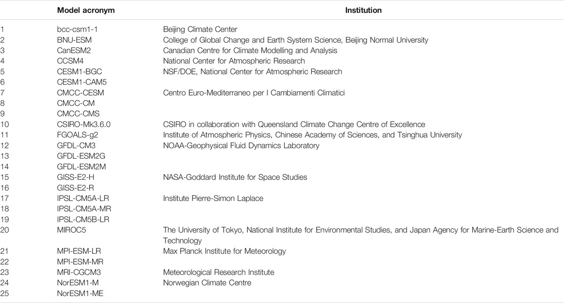
TABLE 1. A list of the CMIP5 models analyzed in this study.

Analysis Procedures

To obtain and isolate the radiative effects of the forcing and feedbacks on the TOA, atmospheric, and surface energy budgets the Fu-Liou radiative transfer mode (RTM; Fu and Liou 1992, 1993) is used for all offline radiative flux calculations at each longitude-latitude grid point of the model using the 50-year monthly mean outputs from the CMIP5 historical and RCP8.5 climate simulations. The radiative flux change at the TOA, atmosphere, and surface due to a specific process (e.g. water vapor change) is calculated by taking the perturbed 50-year monthly mean field of the process in question from the RCP8.5 simulations, with all other variables being held to their 50-year monthly mean fields from the historical simulations, and using these fields as input in our offline radiative flux calculations; then the historical radiative flux is subtracted from the perturbed offline radiative flux giving the radiative flux change due to that process alone, consistent with the PRP approach. As an extension of the PRP approach, similar to the radiative kernel technique, the partial derivatives in the above equations are obtained with the offline radiative transfer model by individually perturbing the temperature in each layer ‘j’ by 1 K and calculating the perturbed radiative flux at the TOA, atmosphere, and surface due to the 1 K increase of that specific layer alone; then as before the unperturbed radiative flux is subtracted from the perturbed offline radiative flux giving the approximate value of the partial derivative. The monthly-mean calculations are then annually averaged, from which the analysis follows.

The use of time-mean fields and a different RTM (i.e., the Fu-Liou RTM) than that native to the CMIP5 models to calculate the offline radiative fluxes introduces an error that is distinct from the linearization error. Previous studies indicate that the use of time-mean cloud fields accounts for most of this error (Sejas et al., 2014; Song et al., 2014a). Song et al. (2014a) found that accounting for the diurnal cycle using hourly data greatly reduced the error introduced by time-mean cloud fields. Supplementary Figure S1 shows there are non-negligible differences between the net radiative flux changes outputted by the CMIP5 models (left column in Supplementary Figure S1) and that calculated with the Fu-Liou RTM using time-mean fields (middle column in Supplementary Figure S1). The linearization error, however, is small, as the linearized version of the net radiative flux changes (right column in Supplementary Figure S1) is quite similar to the non-linearized version given by the Fu-Liou RTM (middle column in Supplementary Figure S1).

The non-radiative terms (e.g., thermodynamics, convection, large-scale dynamics, etc…) are not decomposed in this study, primarily because the energy flux changes due to non-radiative processes are generally not part of the standard CMIP5 data output. In addition, the CMIP5 present and future climate states are not in equilibrium indicating the ocean heat storage is non-negligible. Therefore, we calculate the combined net energy flux changes of the non-radiative terms and heat storage as a residual, taking advantage of the energy budget Eqs 1, 6, 8:

$\begin{array}{c}\Delta Dy{n}_{trans}-\Delta \frac{\partial E_{TOA}}{\partial t}=-\left(\text{Δ}{S}_{TOA}-\text{Δ}{R}_{TOA}\right)\\ \Delta Q_{atm}^{non-rad}-\Delta \left(\frac{\partial E_{atm}}{\partial t}\right)=-\left(\Delta S_{atm}-\Delta R_{atm}\right)\\ \Delta Q_s^{non-rad}-\Delta \left(\frac{\partial E_s}{\partial t}\right)=-\left(\Delta S_s-\Delta R_s\right)\end{array}.(16)$

As indicated by (16), the TOA, atmospheric, and surface net energy flux changes of the non-radiative plus heat storage term are given by the negative sign of the corresponding net radiative energy flux changes.

Results

Energy Flux Changes

Global-Mean

Figure 1 shows the net global-mean energy flux changes at the TOA, atmosphere, and surface due to individual processes. Though, the CMIP5 RCP8.5 simulations are not forced solely by CO₂, the contributions of other well-mixed greenhouse gases (e.g., methane), solar forcing, and aerosol forcing are negligible relative to CO₂ forcing and therefore not shown. The CO₂ forcing in the atmosphere and the surface are positive and approximately equal, meaning the TOA forcing is about twice as large as the surface forcing. The energy flux changes due to water vapor and surface albedo are positive, have similar spreads, and have very small differences between their TOA and surface contributions, as their atmospheric contribution is near-zero. The TOA energy flux change due to non-radiative processes plus heat storage, which is non-zero for a non-equilibrium state, has the same sign as the corresponding surface contribution but with a smaller magnitude due to the partial offset by the positive contribution in the atmosphere. The (net) temperature contributions at the surface and atmosphere are also very similar but negative; the temperature contribution at the TOA is thus substantially more negative and with a greater inter-model spread.

FIGURE 1

FIGURE 1. The global-mean net energy flux changes (W*m⁻²) between the CMIP5 RCP8.5 and historical simulations at the TOA, atmosphere, and surface due to changes in CO₂, water vapor (WV), clouds (CLD), the shortwave (CSW) and longwave (CLW) cloud components, surface albedo (ALB), dynamics plus heat storage (D + HS), and temperature (T). Temperature feedback (T) is further divided into lapse-rate (LR) and Planck (PL) feedbacks at the TOA, and atmospheric (Tatm) and surface (Tsfc) temperature feedbacks in the atmosphere and surface. Note that the sum of the surface and atmosphere contributions equals their respective TOA contributions, except for the last two terms on the right. Black circles indicate individual CMIP5 model results, while red crosses show the CMIP5 ensemble mean.

The cloud contribution at the surface can be positive or negative depending on the model, producing a slightly positive ensemble mean value (∼0.6 W*m⁻²). For nearly all models the TOA cloud contribution is positive and resembles the atmospheric cloud contribution more than the surface, which has a smaller spread. The difference between the TOA and surface cloud contribution is due to the LW cloud component, as the SW component is nearly the same for the TOA and surface. Overall, though, the surface and TOA global-mean results provide a very similar qualitative understanding of process contributions to surface warming.

Zonal-Mean

Unlike the global-mean, more noticeable differences are observed between the TOA and surface perspectives in the zonal-mean. The CO₂ TOA forcing is largest in the tropics and decreases towards the poles, while the surface CO₂ forcing is smallest in the tropics and increases poleward (Figure 2A). The difference is explained by the atmospheric CO₂ forcing, which is positive and larger than the CO₂ surface forcing in the tropics and decreases towards the poles even becoming negative in the Southern Hemisphere polar region. The TOA CO₂ forcing is thus more indicative of the atmospheric than surface forcing. Additionally, the CO₂ forcing has a larger inter-model spread at the TOA than surface. On the other hand, the water vapor TOA energy flux change is more indicative of the surface than atmospheric water vapor energy flux change (Figure 2B). This is a consequence of the atmospheric water vapor net energy flux change being smaller in magnitude than the surface. The negative atmospheric water vapor energy flux change in polar regions does cause the TOA water vapor energy flux change to decrease more from the tropics to poles than at the surface. The albedo TOA energy flux change is nearly the same as that at the surface (Figure 2C). This is because the albedo atmospheric energy flux changes, though slightly negative, are relatively very small. Both perspectives show a large inter-model spread for water vapor and surface albedo feedbacks, particularly in the tropics for the former and in polar regions for the latter. The TOA energy flux change pattern due to (atmospheric and surface) temperature changes is similar to that at the surface (Figure 2D) but is much more negative in the tropics and midlatitudes due to the large negative contribution by the atmospheric component there. The inter-model spread is much greater at the TOA than surface, except in polar regions.

FIGURE 2

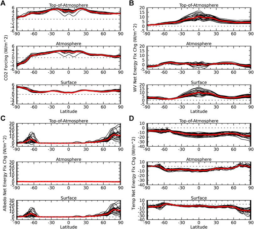
FIGURE 2. The zonal-mean net energy flux change (W*m⁻²) at the TOA, atmosphere, and surface due exclusively to changes in (A) CO₂, (B) water vapor, (C) surface albedo, (D) and temperature. The sum of the surface and atmosphere contributions equals their respective TOA contributions. Individual CMIP5 models (black lines); CMIP5 ensemble mean (red lines).

The energy flux changes due to non-radiative processes and heat storage tend to be negative at the surface but positive in the atmosphere (Figure 3A). This offset leads to a TOA contribution that has a similar pattern to the surface contribution but with a much weaker amplitude. Additionally, the non-radiative TOA energy flux change is positive in the Southern Hemisphere polar region in opposition to the sign of the surface contribution. Both perspectives show a large inter-model spread for this term, though the spread at the TOA is larger, particularly in the Arctic. The meridional pattern and magnitude of the TOA cloud energy flux changes, on the other hand, is more indicative of the atmospheric than surface component, except in the Arctic where the negative atmospheric contribution is canceled by the positive surface contribution (Figure 3B). This is because the SW and LW cloud contributions at the surface offset each other except in the Arctic, where the large positive LW cloud contribution dominates the relatively small negative SW cloud contribution (Figures 3C,D). The atmospheric cloud contribution is dominated by its LW component, as its SW contribution is very small, indicating that the atmospheric LW cloud contribution is mainly responsible for the TOA cloud energy flux changes, excluding the Arctic. The inter-model spread of the cloud feedback is larger at the TOA than surface, mainly due to its LW component. The SW cloud component, however, has a larger spread than its LW component for both perspectives.

FIGURE 3

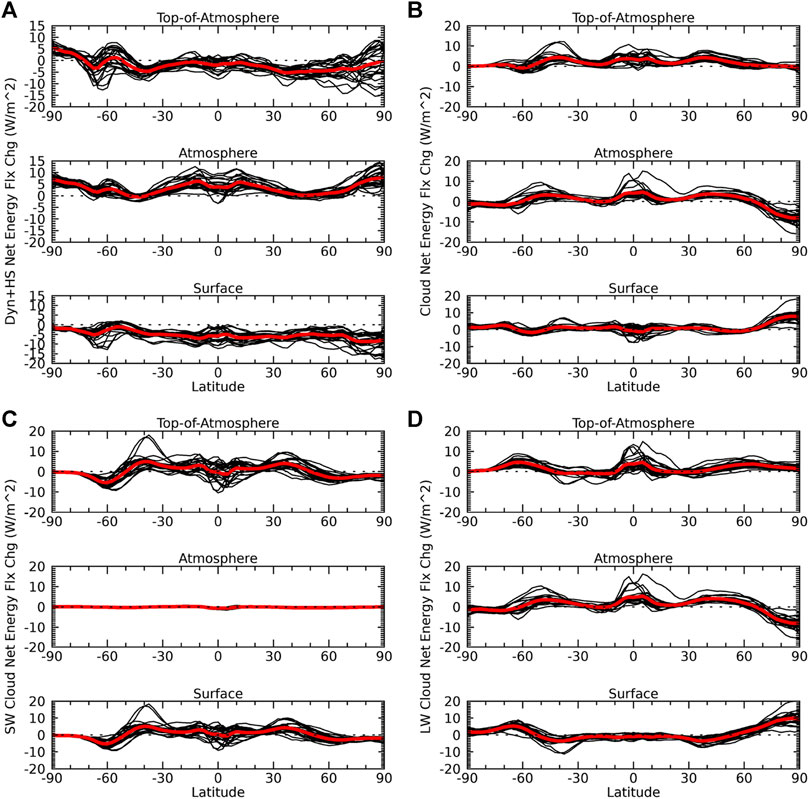
FIGURE 3. Same as Figure 2 but due to changes in (A) dynamics plus heat storage, (B) clouds, and the (C) shortwave and (D) longwave cloud components.

Reconciliation

Thus far the net energy flux changes due to the lapse-rate feedback have not been discussed. The lapse-rate feedback represents the impacts of the deviation from a uniform atmospheric-surface temperature change (equal to the surface temperature change). As indicated by previous studies, the lapse-rate feedback is a manifestation of multiple processes that produce the non-uniform warming response (Cai and Lu 2009; Cronin and Jansen 2016; Feldl et al., 2020; Henry and Merlis 2020; Boeke and Sejas, 2021). As shown in Figures 1–3, the energy flux changes due to radiative and non-radiative processes are not uniform in nature. Therefore, radiative and non-radiative processes naturally produce a non-uniform temperature response. The impact of this non-uniform response on the TOA energy budget is precisely what is taken into account with the lapse-rate feedback. If we could quantify the contribution of individual processes to the lapse-rate feedback and combine it with their corresponding direct impacts on the TOA energy budget, we could obtain the net contribution of radiative and non-radiative processes to the TOA energy flux perturbations.

The CFRAM provides a 3-dimensional picture of radiative and non-radiative process contributions to the surface and atmospheric temperature change. Therefore, we leverage the CFRAM to quantify the contributions of radiative and non-radiative processes to the lapse-rate feedback (Eq. 12) and add it to their corresponding direct energy flux change Eq. 14. As originally shown by Sejas and Cai (2016), we can also quantify the contributions of radiative and non-radiative processes to the atmospheric temperature feedback in the surface perspective Eq. 13. Similarly, these can be combined with the corresponding direct impacts of radiative and non-radiative processes on the surface energy budget Eq. 15. Taking into account the impact of radiative and non-radiative processes on the lapse-rate and atmospheric temperature feedbacks should provide a more consistent picture of process contributions to surface warming, as given by the TOA and surface perspectives.

Global-Mean

Process contributions to the global-mean lapse-rate feedback are shown in Figure 4 (top-left). Non-radiative processes plus ocean heat storage are shown to be the cause of the negative lapse-rate feedback, as greater moist convection enhances upper tropospheric warming and ocean heat storage suppresses surface warming. It is also the source of greatest uncertainty for the lapse-rate feedback. We also find that water vapor feedback is the greatest reducer of the negative lapse-rate feedback (i.e., positive lapse-rate contribution), consistent with the well-known compensation between the two (Cess 1975; Zhang et al., 1994; Soden and Held 2006; Held and Shell 2012; Pendergrass and Hartmann 2014). Adding the decomposed lapse-rate feedback contributions to their corresponding direct TOA contributions (Figure 1), we find carbon dioxide, water vapor, and albedo contributions increase at the TOA, while the non-radiative plus heat storage contribution substantially decreases (Figure 4, top-right). The TOA cloud contribution experiences a very small change as the slight SW increase is offset by the slight LW decrease. Overall, the inter-model spread of all terms increases, particularly the water vapor and non-radiative plus heat storage terms.

FIGURE 4

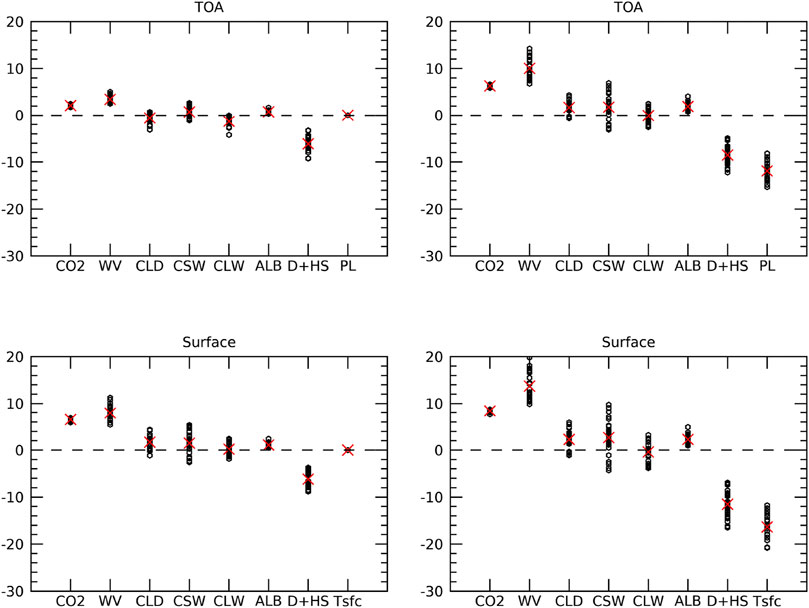
FIGURE 4. The global-mean decomposition of the net energy flux change (W*m⁻²) due to the lapse-rate feedback at the TOA (upper-left) and due to the atmospheric temperature feedback at the surface (bottom-left). The sum of the left column with the corresponding direct impacts of CO₂ (CO2), water vapor (WV), clouds (CLD), SW clouds (CSW), LW clouds (CLW), surface albedo (ALB), dynamics plus heat storage (D + HS), Planck (PL), and surface temperature (Tsfc) given in Figure 1 provides the total contribution of these processes at the TOA (upper-right) and surface (bottom-right), respectively. Black circles indicate individual CMIP5 model results, while red crosses show the CMIP5 ensemble mean.

The warming of the atmosphere enhances the downward LW emission to the surface and thus represents a positive feedback (Figure 1). The decomposition of the atmospheric temperature feedback indicates that the water vapor feedback is the largest contributor to the positive atmospheric temperature feedback with the non-radiative plus heat storage term serving as the largest suppressor (Figure 4, bottom-left); the reverse of the lapse-rate feedback decomposition. Adding the decomposed atmospheric temperature feedback contribution to their corresponding direct surface contributions (Figure 4, bottom-right) increases the magnitude of all process contributions to the surface energy budget. The surface cloud contribution increases mainly as a result of the SW component increasing. The inter-model spread substantially increases for all terms as well, even more than at the TOA.

As shown in Figure 4 (right-panel), including the lapse-rate and atmospheric temperature contributions in the TOA and surface radiative and non-radiative net energy flux changes, respectively, does provide a much more consistent picture between the two perspectives. Both perspectives indicate water vapor feedback is the largest contributor to surface warming, though with large inter-model spread, followed by the CO₂ forcing. Negative energy flux changes due to non-radiative processes plus heat storage are the strongest suppressors of the surface warming and also exhibit large inter-model spread. The largest decrease in net energy flux at the TOA and surface, though, is due to the Planck feedback and surface temperature change, respectively, as these depict the increase in LW emission due to surface warming. Since these two factors are manifestations of the surface warming response itself and its inter-model spread, they do not amplify or suppress the surface warming but instead show how the climate system seeks to balance the positive energy flux perturbations by increasing LW emission through surface warming.

Zonal-Mean

The consistency between the TOA and surface individual process contributions in the zonal-mean is also greatly improved when taking into account their lapse-rate and atmospheric temperature feedback contributions (Figures 5–8). The contributions of the CO₂ forcing to the lapse-rate and atmospheric temperature feedbacks (Figure 5A) are positive like its direct contributions (Figure 2A), but the meridional patterns are reversed. Their addition (Figure 2A plus Figure 5A) leads to a more positive CO₂ forcing for both perspectives, flattens the meridional gradient at the TOA, and flips the sign of the meridional gradient at the surface (Figure 5B). On the other hand, the contributions of water vapor feedback to the lapse-rate and atmospheric temperature feedbacks (Figure 5C) are more similar to their direct contributions (Figure 2B). The water vapor feedback contribution to the lapse-rate feedback, however, displays a meridional gradient that decreases from the tropics to mid-latitudes but then increases in the Arctic. Water vapor feedback is thus an important contributor to the positive lapse-rate feedback in the Arctic, consistent with previous studies (Song et al., 2014b; Henry and Merlis, 2020). The total water vapor feedback contribution (Figure 5D), though, does decrease from the tropics to poles, but with a greater magnitude and inter-model spread, particularly at the surface. Both perspectives indicate water vapor feedback is the largest positive feedback in the tropics.

FIGURE 5

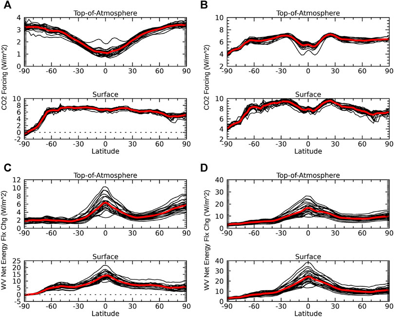
FIGURE 5. The contributions of the (A) CO₂ forcing and (C) water vapor feedback to the net energy flux change (W*m⁻²) associated with the lapse-rate and atmospheric temperature feedbacks at the TOA and surface, respectively. The sum of (A) and (C) with their direct effects (Figures 2A,B, respectively) gives the total energy flux change (W*m⁻²) due to the (b) CO₂ forcing and (d) water vapor feedback at the TOA and surface. Individual CMIP5 models (black lines); CMIP5 ensemble mean (red lines).

FIGURE 6

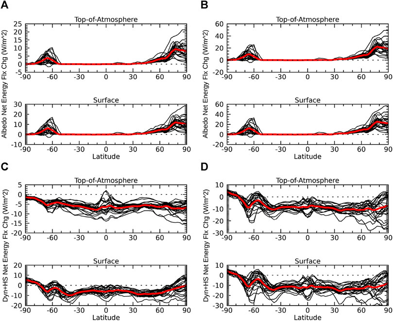
FIGURE 6. Same as Figure 5 but due to changes in surface albedo and dynamics plus heat storage.

FIGURE 7

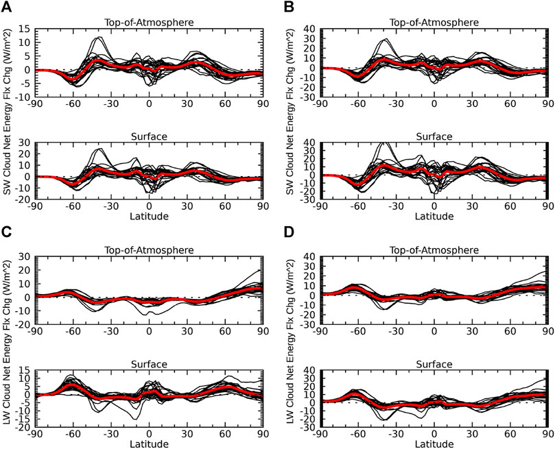
FIGURE 7. Same as Figure 5 but due to the shortwave and longwave cloud feedbacks.

FIGURE 8

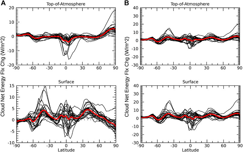
FIGURE 8. Same as Figure 5 but due to the net cloud feedback.

The contributions of surface albedo feedback to the lapse-rate and atmospheric temperature feedbacks (Figure 6A) are very similar to their respective direct contributions (Figure 2C). In line with past studies, we find the surface albedo feedback is the largest contributor to the positive lapse-rate (Graversen et al., 2014; Song et al., 2014b; Feldl et al., 2020) and atmospheric temperature feedbacks (Sejas and Cai 2016) in polar regions, particularly the Arctic. Like its direct contributions, the total surface albedo feedback continues to display no difference between the two perspectives (Figure 6B). However, the inclusion of the lapse-rate and atmospheric temperature contributions does increase the magnitude and inter-model spread of the surface albedo feedback in polar regions (Figures 6B vs. 2C), where both perspectives indicate the surface albedo feedback is the largest positive feedback.

The contribution of the non-radiative plus heat storage term to the lapse-rate feedback (Figure 6C) shows that it is responsible for the negative lapse-rate feedback in the tropics, consistent with the connection between moist convection and the lapse-rate feedback outlined in previous studies (Hansen et al., 1997; Sobel et al., 2001; Cronin and Jansen 2016), and suppresses the positive lapse-rate feedback in polar regions due to ocean heat storage. At the surface, the contribution of the non-radiative plus heat storage term to the atmospheric temperature feedback is largely negative except in the Antarctic; in the Arctic the inter-model uncertainty is very large with differing sign among models (Figure 6C). The total non-radiative plus heat storage contribution tends to be negative with a similar meridional pattern relative to its direct contributions at both the TOA and surface (Figures 6D ve. 3A), but the negative contribution and inter-model spreads are much larger. We also find the surface contribution is now positive in the Antarctic matching the TOA perspective.

The SW cloud feedback contributions to the lapse-rate and atmospheric temperature feedbacks matches its direct contributions (Figure 7A); its addition just amplifies the magnitude and inter-model spread of the direct contributions (Figure 7B). On the other hand, the LW cloud feedback contributions to the lapse-rate and atmospheric temperature feedbacks do not match its direct contributions (Figure 7C). The LW cloud feedback contributes to both the negative and positive lapse-rate feedback in the tropics and polar regions, respectively. At the surface, the LW cloud feedback tends to contribute positively to the atmospheric temperature feedback, though there is large inter-model uncertainty. The total LW cloud feedback displays less inter-model spread at the TOA, but more inter-model spread at the surface (Figures 7D vs. 3D). Though there is substantial offsetting between the LW and SW cloud feedbacks in the ensemble mean, the SW cloud feedback tends to dominate everywhere, except in the Arctic; thus, leading to a slight increase in the magnitude and inter-model spread of the net cloud feedback relative to its direct contributions (Figures 8B vs 3B).

Discussion

In this study we compared the surface and TOA energy budget decompositions used to attribute surface warming to individual process contributions. We show that the differences between the two methodologies are explained by non-negligible changes to the atmospheric energy budget. In the global-mean, the impact of the atmospheric energy flux perturbations due to individual processes is smaller or of the same sign as the corresponding surface energy flux perturbations such that the TOA and surface perspectives provide a similar qualitative understanding. However, when expanding to a zonal-mean analysis, differences in pattern and even sign become apparent. This is due to individual processes, such as the CO₂ forcing, clouds, dynamics and ocean heat storage, modifying the atmospheric and surface energy budgets very differently. Energy perturbations at the TOA due to individual processes and their inter-model spreads are thus a manifestation of the combined inter-model uncertainty and impacts of these processes on the atmospheric and surface energy budgets. When the magnitude of the atmospheric energy flux perturbation due to a specific process is large and pattern different than the energy flux perturbation it causes at the surface, the TOA and surface energy budget perturbations due to that process will differ greatly.

The asymmetry between the atmospheric and surface energy flux perturbations is precisely what is taken into account with the lapse-rate feedback. When we decompose the lapse-rate feedback at the TOA and the atmospheric temperature feedback at the surface into contributions by individual processes and add it to their corresponding direct effects a much more consistent picture between the two perspectives is achieved. Though differences in magnitude persist, the modified decomposition provides the same qualitative understanding of the inter-model spread, spatial pattern, and sign of the individual process contributions for both perspectives. Moreover, the relative importance of individual contributions to surface warming are in agreement.

With the modified approach, both perspectives indicate water vapor feedback is the largest contributor in the tropics, while surface albedo feedback is the greatest contributor in polar regions. Dynamics and ocean heat storage are the main suppressors of surface warming, except over Antarctica. Both perspectives show there is large inter-model uncertainty in the contributions of water vapor, clouds, albedo, and dynamics plus ocean heat storage. How these uncertainties amplify or offset each other and thus contribute to the inter-model warming spread is beyond the scope of this paper. However, the large inter-model spread in the dynamics plus ocean heat storage term does present a possible source of uncertainty hidden within the lapse-rate feedback that is often overlooked.

We note that our TOA energy budget decomposition uses the instantaneous instead of the stratospheric-adjusted radiative forcing. Since the stratosphere cools, its main impact is the reduction (increase) in magnitude of the negative (positive) lapse-rate feedback in the tropics (Arctic). This is mainly compensated by the global decrease in the CO₂ forcing (i.e., instantaneous vs stratospheric-adjusted radiative forcing), since CO₂ forcing is the predominant cause of stratospheric cooling (Fels et al., 1980). The total CO₂ forcing (i.e., including its contribution to the lapse-rate feedback) takes this compensation into account such that the total CO₂ forcing effectively includes stratospheric adjustment.

The non-negligible error, due to the use of time-mean fields in our offline radiative calculations, will impact some of the details in our analysis (Supplementary Figure S1). The error, however, is unlikely to change our main conclusions as indicated by previous studies (Sejas et al., 2014; Song et al., 2014a). More importantly, the ability to reconcile the TOA and surface process contributions to surface warming through decompositions of the lapse-rate and atmospheric temperature feedbacks is not dependent on the offline error.

The reconciliation of the TOA and surface perspectives relies on a decomposition made solely possible by the 3-dimensional CFRAM analysis. The need to carry out a 3-dimensional CFRAM analysis, however, detracts from the simplicity provided by the TOA methodology. Therefore, if using a TOA approach, it is important to understand that the differences in interpretation are due to process contributions hidden within the lapse-rate feedback. Alternatively, one could solely use the CFRAM to study radiative and non-radiative process contributions to surface and atmospheric warming and the inter-model warming spread (Cai and Tung 2012; Taylor et al., 2013; Sejas et al., 2014; Song et al., 2014a; Yoshimori et al., 2014; Hu et al., 2020).

Data Availability Statement

Publicly available datasets were analyzed in this study. This data can be found here: http://data.ceda.ac.uk/badc/cmip5/data/cmip5/ and https://esgf-node.llnl.gov/search/cmip5/. The RCP forcing database is freely accessible at https://tntcat.iiasa.ac.at/RcpDb/.

Author Contributions

SS conceived the idea for this study, analyzed the data, and was the lead writer. MC, XH, and HF helped with the writing of the manuscript. XH and HF downloaded the CMIP5 data and carried out the CFRAM analysis. All authors discussed the results and provided input throughout the study.

Funding

This study was supported by the National Natural Science Foundation of China (Grants 41690123, 41690120, and 41805050), the Natural Science Foundation of Guangdong Province of China (Grant 2018A0303130268), and the National Science Foundation (AGS-2012479).

Conflict of Interest

SS is employed by the company Science Systems and Applications Inc.

The remaining authors declare that the research was conducted in the absence of any commercial or financial relationships that could be construed as a potential conflict of interest.

Publisher’s Note

All claims expressed in this article are solely those of the authors and do not necessarily represent those of their affiliated organizations, or those of the publisher, the editors and the reviewers. Any product that may be evaluated in this article, or claim that may be made by its manufacturer, is not guaranteed or endorsed by the publisher.

Supplementary Material

The Supplementary Material for this article can be found online at: https://www.frontiersin.org/articles/10.3389/feart.2021.725816/full#supplementary-material

References

Aires, F., and Rossow, W. B. (2003). Inferring Instantaneous, Multivariate and Nonlinear Sensitivities for the Analysis of Feedback Processes in a Dynamical System: Lorenz Model Case-Study. Q. J. R. Meteorol. Soc. 129, 239–275. doi:10.1256/qj.01.174

CrossRef Full Text | Google Scholar

Andrews, T., Forster, P. M., and Gregory, J. M. (2009). A Surface Energy Perspective on Climate Change. J. Clim. 22, 2557–2570. doi:10.1175/2008JCLI2759.1

CrossRef Full Text | Google Scholar

Bates, J. R. (2007). Some Considerations of the Concept of Climate Feedback. Q.J.R. Meteorol. Soc. 133, 545–560. doi:10.1002/qj.62

CrossRef Full Text | Google Scholar

Boeke, R. C., and Taylor, P. C. (2018). Seasonal Energy Exchange in Sea Ice Retreat Regions Contributes to Differences in Projected Arctic Warming. Nat. Commun. 9, 5017. doi:10.1038/s41467-018-07061-9

PubMed Abstract | CrossRef Full Text | Google Scholar

Boeke, R. C., Taylor, P. C., and Sejas, S. A. (2021). On the Nature of the Arctic's Positive Lapse‐Rate Feedback. Geophys. Res. Lett. 48, e2020GL091109. doi:10.1029/2020GL091109

CrossRef Full Text | Google Scholar

Bony, S., Colman, R., Kattsov, V. M., Allan, R. P., Bretherton, C. S., Dufresne, J.-L., et al. (2006). How Well Do We Understand and Evaluate Climate Change Feedback Processes? J. Clim. 19, 3445–3482. doi:10.1175/jcli3819.1

CrossRef Full Text | Google Scholar

Cai, M., and Lu, J. (2009). A New Framework for Isolating Individual Feedback Processes in Coupled General Circulation Climate Models. Part II: Method Demonstrations and Comparisons. Clim. Dyn. 32, 887–900. doi:10.1007/s00382-008-0424-4

CrossRef Full Text | Google Scholar

Cai, M., and Tung, K.-K. (2012). Robustness of Dynamical Feedbacks from Radiative Forcing: 2% Solar versus 2 × CO₂ Experiments in an Idealized GCM. J. Atmos. Sci. 69, 2256–2271. doi:10.1175/JAS-D-11-0117.1

CrossRef Full Text | Google Scholar

Cess, R. D. (1975). Global Climate Change: an Investigation of Atmospheric Feedback Mechanisms. Tellus 27, 193–198. doi:10.3402/tellusa.v27i3.9901

CrossRef Full Text | Google Scholar

Cess, R. D., Zhang, M. H., Ingram, W. J., Potter, G. L., Alekseev, V., Barker, H. W., et al. (1996). Cloud Feedback in Atmospheric General Circulation Models: An Update. J. Geophys. Res. 101, 12791–12794. doi:10.1029/96JD00822

CrossRef Full Text | Google Scholar

Colman, R. A. (2015). Climate Radiative Feedbacks and Adjustments at the Earth's Surface. J. Geophys. Res. Atmos. 120, 3173–3182. doi:10.1002/2014JD022896

CrossRef Full Text | Google Scholar

Cronin, T. W., and Jansen, M. F. (2016). Analytic Radiative‐advective Equilibrium as a Model for High‐latitude Climate. Geophys. Res. Lett. 43, 449–457. doi:10.1002/2015GL067172

CrossRef Full Text | Google Scholar

Feldl, N., Anderson, B. T., and Bordoni, S. (2017). Atmospheric Eddies Mediate Lapse Rate Feedback and Arctic Amplification. J. Clim. 30, 9213–9224. doi:10.1175/JCLI-D-16-0706.1

CrossRef Full Text | Google Scholar

Feldl, N., Po-Chedley, S., Singh, H. K. A., Hay, S., and Kushner, P. J. (2020). Sea Ice and Atmospheric Circulation Shape the High-Latitude Lapse Rate Feedback. Npj Clim. Atmos. Sci. 3, 1–9. doi:10.1038/s41612-020-00146-7

CrossRef Full Text | Google Scholar

Fels, S. B., Mahlman, J. D., Schwarzkopf, M. D., and Sinclair, R. W. (1980). Stratospheric Sensitivity to Perturbations in Ozone and Carbon Dioxide: Radiative and Dynamical Response. J. Atmos. Sci. 37, 2265–2297. doi:10.1175/1520-0469(1980)037<2265:sstpio>2.0.co;2

CrossRef Full Text | Google Scholar

Fu, Q., and Liou, K. N. (1992). On the Correlated k -Distribution Method for Radiative Transfer in Nonhomogeneous Atmospheres. J. Atmospheric Sci. 49, 2139–2156.

CrossRef Full Text | Google Scholar

Fu, Q., and Liou, K. N. (1993). Parameterization of the Radiative Properties of Cirrus Clouds. J. Atmospheric Sci. 50, 2008–2025. doi:10.1175/JCLI-D-16-0706.1

CrossRef Full Text | Google Scholar

Goosse, H., Kay, J. E., Armour, K. C., Bodas-Salcedo, A., Chepfer, H., Docquier, D., et al. (2018). Quantifying Climate Feedbacks in Polar Regions. Nat. Commun. 9, 1919. doi:10.1038/s41467-018-04173-0

PubMed Abstract | CrossRef Full Text | Google Scholar

Graversen, R. G., Langen, P. L., and Mauritsen, T. (2014). Polar Amplification in CCSM4: Contributions from the Lapse Rate and Surface Albedo Feedbacks. J. Clim. 27, 4433–4450. doi:10.1175/JCLI-D-13-00551.1

CrossRef Full Text | Google Scholar

Gregory, J. M., Ingram, W. J., Palmer, M. A., Jones, G. S., Stott, P. A., Thorpe, R. B., et al. (2004). A New Method for Diagnosing Radiative Forcing and Climate Sensitivity. Geophys. Res. Lett. 31, L03205. doi:10.1029/2003GL018747

CrossRef Full Text | Google Scholar

Hansen, J., Sato, M., and Ruedy, R. (1997). Radiative Forcing and Climate Response. J. Geophys. Res. 102, 6831–6864. doi:10.1029/96JD03436

CrossRef Full Text | Google Scholar

Hartmann, D. L., Klein Tank, A. M. G., and Rusticucci, M. (2013). “Observations: Atmosphere and Surface,” in Climate Change 2013: The Physical Science Basis. Contribution of Working Group I to the Fifth Assessment Report of the IPCC (Cambridge, UK, and New York, NY, USA: Cambridge University Press).

Google Scholar

Held, I. M., and Shell, K. M. (2012). Using Relative Humidity as a State Variable in Climate Feedback Analysis. J. Clim. 25, 2578–2582. doi:10.1175/JCLI-D-11-00721.1

CrossRef Full Text | Google Scholar

Henry, M., and Merlis, T. M. (2020). Forcing Dependence of Atmospheric Lapse Rate Changes Dominates Residual Polar Warming in Solar Radiation Management Climate Scenarios. Geophys. Res. Lett. 47, e2020GL087929. doi:10.1029/2020GL087929

CrossRef Full Text | Google Scholar

Hu, X., Cai, M., Yang, S., and Sejas, S. A. (2018). Air Temperature Feedback and its Contribution to Global Warming. Sci. China Earth Sci. 61, 1491–1509. doi:10.1007/s11430-017-9226-6

CrossRef Full Text | Google Scholar

Hu, X., Fan, H., Cai, M., Sejas, S. A., Taylor, P., and Yang, S. (2020). A Less Cloudy Picture of the Inter-model Spread in Future Global Warming Projections. Nat. Commun. 11, 4472. doi:10.1038/s41467-020-18227-9

PubMed Abstract | CrossRef Full Text | Google Scholar

IPCC (2013). Climate Change 2013: The Physical Science Basis. Contribution of Working Group I to the Fifth Assessment Report of the IPCC [Stocker, T. F., D. Qin, G.-K. Plattner, M. Tignor, S. K. Allen, J. Boschung, A. Nauels, Y. Xia, V. Bex and P. M. Midgley (eds.)], Cambridge, UK, and New York, NY: Cambridge University Press, 1535.

Google Scholar

Klocke, D., Quaas, J., and Stevens, B. (2013). Assessment of Different Metrics for Physical Climate Feedbacks. Clim. Dyn. 41, 1173–1185. doi:10.1007/s00382-013-1757-1

CrossRef Full Text | Google Scholar

Kramer, R. J., He, H., Soden, B. J., Oreopoulos, L., Myhre, G., Forster, P. M., et al. (2021). Observational Evidence of Increasing Global Radiative Forcing. Geophys. Res. Lett. 48, e2020GL091585. doi:10.1029/2020GL091585

CrossRef Full Text | Google Scholar

Lahellec, A., and Dufresne, J.-L. (2013). A Formal Analysis of the Feedback Concept in Climate Models. Part I: Exclusive and Inclusive Feedback Analyses*. J. Atmos. Sci. 70, 3940–3958. doi:10.1175/JAS-D-12-0218.1

CrossRef Full Text | Google Scholar

Lahellec, A., and Dufresne, J.-L. (2014). A Formal Analysis of the Feedback Concept in Climate Models. Part II: Tangent Linear Systems in GCMs. J. Atmos. Sci. 71, 3350–3375. doi:10.1175/JAS-D-13-0334.1

CrossRef Full Text | Google Scholar

Laîné, A., Yoshimori, M., and Abe-Ouchi, A. (2016). Surface Arctic Amplification Factors in CMIP5 Models: Land and Oceanic Surfaces and Seasonality. J. Clim. 29, 3297–3316. doi:10.1175/JCLI-D-15-0497.1

CrossRef Full Text | Google Scholar

Lu, J., and Cai, M. (2009a). A New Framework for Isolating Individual Feedback Processes in Coupled General Circulation Climate Models. Part I: Formulation. Clim. Dyn. 32, 873–885. doi:10.1007/s00382-008-0425-3

CrossRef Full Text | Google Scholar

Lu, J., and Cai, M. (2009b). Seasonality of Polar Surface Warming Amplification in Climate Simulations. Geophys. Res. Lett. 36, L16704. doi:10.1029/2009GL040133

CrossRef Full Text | Google Scholar

Manabe, S., Stouffer, R. J., Spelman, M. J., and Bryan, K. (1991). Transient Responses of a Coupled Ocean-Atmosphere Model to Gradual Changes of Atmospheric CO2. Part I. Annual Mean Response. J. Clim. 4, 785–818. doi:10.1175/1520-0442(1991)004<0785:TROACO>2.0.CO;2

CrossRef Full Text | Google Scholar

Manabe, S., and Wetherald, R. T. (1975). The Effects of Doubling the CO2Concentration on the Climate of a General Circulation Model. J. Atmos. Sci. 32, 3–15. doi:10.1175/1520-0469(1975)032<0003:TEODTC>2.0.CO;2

CrossRef Full Text | Google Scholar

Payne, A. E., Jansen, M. F., and Cronin, T. W. (2015). Conceptual Model Analysis of the Influence of Temperature Feedbacks on Polar Amplification. Geophys. Res. Lett. 42, 9561–9570. doi:10.1002/2015GL065889

CrossRef Full Text | Google Scholar

Pendergrass, A. G., and Hartmann, D. L. (2014). The Atmospheric Energy Constraint on Global-Mean Precipitation Change. J. Clim. 27, 757–768. doi:10.1175/JCLI-D-13-00163.1

CrossRef Full Text | Google Scholar

Pithan, F., and Mauritsen, T. (2014). Arctic Amplification Dominated by Temperature Feedbacks in Contemporary Climate Models. Nat. Geosci 7, 181–184. doi:10.1038/ngeo2071

CrossRef Full Text | Google Scholar

Previdi, M., and Liepert, B. G. (2012). The Vertical Distribution of Climate Forcings and Feedbacks from the Surface to Top of Atmosphere. Clim. Dyn. 39, 941–951. doi:10.1007/s00382-011-1233-8

CrossRef Full Text | Google Scholar

Robock, A. (1983). Ice and Snow Feedbacks and the Latitudinal and Seasonal Distribution of Climate Sensitivity. J. Atmos. Sci. 40, 986–997. doi:10.1175/1520-0469(1983)040<0986:iasfat>2.0.co;2

CrossRef Full Text | Google Scholar

Schlesinger, M. E., and Mitchell, J. F. B. (1987). Climate Model Simulations of the Equilibrium Climatic Response to Increased Carbon Dioxide. Rev. Geophys. 25, 760–798. doi:10.1029/RG025i004p00760

CrossRef Full Text | Google Scholar

Sejas, S. A., Cai, M., Hu, A., Meehl, G. A., Washington, W., and Taylor, P. C. (2014). Individual Feedback Contributions to the Seasonality of Surface Warming. J. Clim. 27, 5653–5669. doi:10.1175/JCLI-D-13-00658.1

CrossRef Full Text | Google Scholar

Sejas, S. A., and Cai, M. (2016). Isolating the Temperature Feedback Loop and its Effects on Surface Temperature. J. Atmos. Sci. 73, 3287–3303. doi:10.1175/JAS-D-15-0287.1

CrossRef Full Text | Google Scholar

Sobel, A. H., Nilsson, J., and Polvani, L. M. (2001). The Weak Temperature Gradient Approximation and Balanced Tropical Moisture Waves*. J. Atmos. Sci. 58, 3650–3665. doi:10.1175/1520-0469(2001)058<3650:TWTGAA>2.0.CO;2

CrossRef Full Text | Google Scholar

Soden, B. J., Broccoli, A. J., and Hemler, R. S. (2004). On the Use of Cloud Forcing to Estimate Cloud Feedback. J. Clim. 17, 3661–3665. doi:10.1175/1520-0442(2004)017<3661:OTUOCF>2.0.CO;2

CrossRef Full Text | Google Scholar

Soden, B. J., and Held, I. M. (2006). An Assessment of Climate Feedbacks in Coupled Ocean-Atmosphere Models. J. Clim. 19, 3354–3360. doi:10.1175/jcli3799.1

CrossRef Full Text | Google Scholar

Soden, B. J., Held, I. M., Colman, R., Shell, K. M., Kiehl, J. T., and Shields, C. A. (2008). Quantifying Climate Feedbacks Using Radiative Kernels. J. Clim. 21, 3504–3520. doi:10.1175/2007JCLI2110.1

CrossRef Full Text | Google Scholar

Song, X., Zhang, G. J., and Cai, M. (2014a). Characterizing the Climate Feedback Pattern in the NCAR CCSM3-SOM Using Hourly Data. J. Clim. 27, 2912–2930. doi:10.1175/JCLI-D-13-00567.1

CrossRef Full Text | Google Scholar

Song, X., Zhang, G. J., and Cai, M. (2014b). Quantifying contributions of climate feedbacks to tropospheric warming in the NCAR CCSM3.0. Clim. Dyn. 42, 901–917. doi:10.1007/s00382-013-1805-x

CrossRef Full Text | Google Scholar

Stephens, G. L. (2005). Cloud Feedbacks in the Climate System: A Critical Review. J. Clim. 18, 237–273. doi:10.1175/jcli-3243.1

CrossRef Full Text | Google Scholar

Taylor, P. C., Cai, M., Hu, A., Meehl, J., Washington, W., and Zhang, G. J. (2013). A Decomposition of Feedback Contributions to Polar Warming Amplification. J. Clim. 26, 7023–7043. doi:10.1175/JCLI-D-12-00696.1

CrossRef Full Text | Google Scholar

Thorsen, T. J., Kato, S., Loeb, N. G., and Rose, F. G. (2018). Observation-Based Decomposition of Radiative Perturbations and Radiative Kernels. J. Clim. 31, 10039–10058. doi:10.1175/JCLI-D-18-0045.1

CrossRef Full Text | Google Scholar

Washington, W. M., and Meehl, G. A. (1984). Seasonal Cycle experiment on the Climate Sensitivity Due to a Doubling of CO2with an Atmospheric General Circulation Model Coupled to a Simple Mixed-Layer Ocean Model. J. Geophys. Res. 89, 9475–9503. doi:10.1029/JD089iD06p09475

CrossRef Full Text | Google Scholar

Wetherald, R. T., and Manabe, S. (1988). Cloud Feedback Processes in a General Circulation Model. J. Atmos. Sci. 45, 1397–1416. doi:10.1175/1520-0469(1988)045<1397:cfpiag>2.0.co;2

CrossRef Full Text | Google Scholar

Yoshimori, M., Watanabe, M., Abe-Ouchi, A., Shiogama, H., and Ogura, T. (2014). Relative Contribution of Feedback Processes to Arctic Amplification of Temperature Change in MIROC GCM. Clim. Dyn. 42, 1613–1630. doi:10.1007/s00382-013-1875-9

CrossRef Full Text | Google Scholar

Zhang, M. H., Hack, J. J., Kiehl, J. T., and Cess, R. D. (1994). Diagnostic Study of Climate Feedback Processes in Atmospheric General Circulation Models. J. Geophys. Res. 99, 5525–5537. doi:10.1029/93JD03523

CrossRef Full Text | Google Scholar