Investigating Predictability of the TRHR Seasonal Precipitation at Long Lead Times Using a Generalized Regression Model with Regularization

Skillful long-lead climate forecast is of great importance in managing large water systems and can be made possible using teleconnections between regional climate and large-scale circulations. Recent innovations in machine learning provide powerful tools in exploring linear/nonlinear associations between climate variables. However, while it is hard to give physical interpretation of the more complex models, the simple models can be vulnerable to over-fitting, especially when dealing with the highly “non-square” climate data. Here, as a compromise of interpretability and complexity, we proposed a regression model by coupling pooling and a generalized regression with regularization. Performance of the model is tested in estimating the Three-Rivers Headwater Region wet-season precipitation using the sea surface temperatures at lead times of 0–24 months. The model shows better predictive skill for certain long lead times when compared with some commonly used regression methods including the Ordinary Least Squares (OLS), Empirical Orthogonal Function (EOF), and Canonical Correlation Analysis (CCA) regressions. The high skill is found to relate to the persistent regional correlation patterns between the predictand precipitation and predictor SSTs as also confirmed by a correlation analysis. Furthermore, flexibility of the model is demonstrated using a multinomial regression model which shows good skill around the long lead time of 22 months. Consistent clusters of SSTs are found to contribute to both models. Two SST indices are defined based on the major clusters of predictors and are found to be significantly correlated with the predictand precipitation at corresponding lead times. In conclusion, the proposed regression model demonstrates great flexibility and advantages in dealing with collinearity while preserving simplicity and interpretability, and shows potential as a cheap preliminary analysis tool to guide further study using more complex models.

1 Introduction

Skillful long-lead (seasonal to annual) climate forecast is of great importance in managing large water systems. Examples include but are not limited to making water transferring plans for multi-reservoir systems running at annual to inter-annual time scales (Carpenter and Georgakakos, 2001; Block, 2011), informing long-term agricultural decision making (Lemos et al., 2002; Hansen et al., 2011), and developing early warning system for disaster mitigation (Wilhite and Svoboda, 2000; Verdin et al., 2005). While local climate variability always fails to persist through such long lead times, the prediction can be made possible using long-lead teleconnections between regional climate and large-scale circulations. Anomalies of large-scale atmospheric circulations can be anchored by ocean memory due to massive heat capacity of ocean water and be released to perturb other circulations at a much later time (Xie et al., 2009; Xie et al., 2016). These perturbations can therefore be indicated by SST anomalies. There are already well-established SST-based climate indices that have seen good use in long-lead climate forecasts such as the Niño SST indices (Rasmusson and Carpenter, 1982; Trenberth, 1997; Trenberth and Stepaniak, 2001), the Pacific Decadal Oscillation (PDO) (Mantua et al., 1997; Zhang et al., 1997), the Tropical Northern Atlantic (TNA) and the Tropical Southern Atlantic (TSA) indices (Enfield et al., 1999) etc.

Approaches commonly used in developing long-term prediction models based on large-scale teleconnections can be roughly categorized into two classes: 1) physically-based simulation and 2) statistical models. While the physically-based simulation is widely used in investigating causality chains of climate processes, it is usually computationally intensive and requires expertise for parameter calibration (Menemenlis et al., 2005; Sahastrabuddhe and Ghosh, 2021). Its statistical counterpart, in the meantime, provides an easy access to examining statistical associations between climate variables which could be further used to develop prediction models. The statistical models are becoming increasingly popular thanks to the advances of sensing technology and internet which makes tremendously more data available at exceptionally high temporal and spatial resolutions (Liu, 2015). Early efforts of statistical modelling are featured by qualitative analysis comparing time series of different climate variables (Thornthwaite, 1948; Von Storch and Zwiers, 2001). Most early work relied on insights of the expert researchers and were done with data of rather limited size. Recent innovations in machine learning have developed powerful tools for examining linear/non-linear associations between climate variables in massive volumes in a more automated way. Just to name a few examples here: Kernelization is used to extend study domain from linear associations to nonlinear associations (Ali et al., 2019; Bueso et al., 2020). Data processing tips like pooling and convolution are used to enhance model robustness by discarding/smoothing noises (Devineni and Sankarasubramanian, 2010; Schepen et al., 2018). Of the many machine learning approaches, neural network has become extremely popular across a wide range of spatial scales (local-global) (Goddard et al., 2001; Mekanik et al., 2013; Fan et al., 2015; Ham et al., 2019; Reichstein et al., 2019). Ham et al. (2019) even successfully extended lead time of skillful ENSO forecast to one and a half years using a convolution neural network trained on historical simulations, which beat many state-of-the-art dynamical systems in terms of correlation skill for the Niño 3.4 Index. However, even though efforts are being made to improve model interpretability (Gilpin et al., 2018; Carvalho et al., 2019; Worland et al., 2019), tools for explaining the machine learning models are still insufficient (Gilpin et al., 2018) and to find physical interpretation of these models is usually hard or even impossible due to high model complexity. In this study, we looked at a generalized regularized regression method (i.e., elastic net) coupled with pooling as a compromise between model interpretability and complexity, and examined its performance in predicting regional seasonal precipitation based on large-scale SST anomalies.

Regression has been broadly used in climate research and related fields. Typical applications include 1) change point detection (Solow, 1987; Mudelsee, 2000), 2) developing forecast models (Krishnamurti et al., 1999; Mekanik et al., 2013; Kharin and Zwiers, 2002), and 3) identification of covariates with high predictive skill (Wakabayashi and Kawamura, 2004; Matsui and Konishi, 2011). Not only can the regression model identify the linear relationships between the climate variables at a given temporal basis (e.g., monthly or annual), but it also has good interpretability for guiding further research using more complex, nonlinear statistical methods or physically-based modeling experiments. These two features make regression especially popular in exploring teleconnections between regional climate and large-scale circulations. Hurrell (1996) used a multivariate linear regression model to link changes in northern hemisphere temperature to extratropical climate indices. Krishnamurti et al. (1999) developed a superensemble method for improving weather and climate forecast skills by using coefficients from multiple regressions. Wakabayashi and Kawamura (2004) extracted four major teleconnection patterns in predicting Japan summer climate anomalies by combining the empirical orthogonal function (EOF) and regression. Van Oldenborgh and Burgers (2005) developed a synthetic precipitation generator with regression models using the Niño 3.4 Index as the sole regressor to examine decadal variation in global ENSO-precipitation teleconnections. Yang and DelSole (2012) used the regression coefficient maps to explore teleconnections between ENSO and different climate fields. More recently, Zhang et al. (2020) examined teleconnections between the Arctic sea ice decline and major climate indices using the quantile regression analysis. Only a few examples are listed here for context, as our intent is to test a generalized regression model with regularization in long-term seasonal precipitation forecast instead of doing a thorough review applications of regression in climate research.

However, over-fitting and over-parameterization are important issues for most regression analysis. These issues are particularly pertinent in climate research, since the remote sensing data are usually highly “non-square” (i.e., the total number of time series largely exceeds the length of the time series). Therefore, it is necessary to reduce the effective dimensionality of the problems. Two commonly used approaches have been: 1) to select only a few predominant features/patterns (e.g., the Principal Component Analysis, PCA (Schoof and Pryor, 2001; Wakabayashi and Kawamura, 2004; Li et al., 2020) or the Canonical Correlation Analysis, CCA (Mo, 2003; Yang and DelSole, 2012)); 2) to use only a few well-established climate indices (Van Oldenborgh and Burgers, 2005; Rust et al., 2015; Tan and Shao, 2017; Zhang et al., 2020). However, both methods have intrinsic disadvantages: Traditional dimensionality reduction methods like PCA and CCA try to decompose the global covariance structure of the predictors (PCA) or between the predictand and the predictors (CCA) and can miss important regional patterns while the climate indices are only defined by prior knowledge and thus could limit the domain where we want to explore the potential teleconnections.

In the past few decades, regularization has become increasingly popular in dealing with multicollinearity in regression. The two regularization approaches commonly used with regression are the L-1 norm (the least absolute shrinkage and selection operator, LASSO (Tibshirani, 1996)) and the L-2 norm (the ridge regression (Hoerl and Kennard, 1970)) of regression coefficients. Other popular regularization approaches include the Akaike’s Information Criterion (AIC) (Akaike, 1998) and the Bayesian Information Criterion (BIC) (Schwarz, 1978). Both L-1 and L-2 norm regularizations have shown good performance in alleviating or avoiding over-fitting in regression models in climate research (Matsui and Konishi, 2011; Soleh et al., 2015; DelSole and Banerjee, 2017; Kim et al., 2017; Li et al., 2020). Yet, it should be noted that the ridge regression does not directly provoke sparsity of the regression model while the LASSO regression tends to assign non-zero value to only one of many correlated predictors which can make the model difficult to interpret. The lack of interpretability of the lasso model is also pointed out in a recent paper from Stevens et al. (2021) where a graph-guided variation is used as an extra regularization to improve robustness of the regression model in predicting Southwestern United States winter precipitation. Here, we propose to use the elastic net regularization (Zou and Hastie, 2005) which linearly combines the LASSO and ridge regression regularizations. While the LASSO regularization guarantees sparsity of the model, the ridge regression regularization helps improve visualization of the regression coefficient map and therefore, interpretability of the model (Peng et al., 2020). On top of that, a pooling layer is added before developing the regression model. The pooling layer is commonly used in machine learning for reducing spatial dimensions (Zeiler and Fergus, 2013; Yu et al., 2014; Kalchbrenner et al., 2014). And this extra pooling layer should help improve robustness of the model by avoiding the realistic problem that major “hot” regions defining large-scale circulations are not fixed to certain spatial grids naturally.

The proposed model is tested to predict the Three-Rivers Headwater Region (TRHR) wet-season precipitation using the Pacific Ocean and Indian Ocean SSTs. The TRHR, located in the eastern Tibetan Plateau (TP), is often called China’s Water Tower as from it flow the three major rivers of China: the Yellow River, the Yangtze River, and the Lancang (Mekong) River. Consequently, the TRHR plays a critical role in providing invaluable ecological goods and serviced as well as other resources like energy and food. While great efforts have been devoted to studying teleconnections between the broader TP precipitation and large-scale climates (Benn and Owen, 1998; Shaman and Tziperman, 2005; Feng and Zhou, 2012; Dong et al., 2020), the quantitative studies focusing solely on the TRHR are rather limited and only looks at short lead times (Zhang et al., 2019; Zhao et al., 2019). In this study, we extend the forecast lead time up to 24 months and the performance are compared against some widely-used regression methods including OLS multi-linear regression, the EOF regression, and the CCA regression. The precipitation is predicted in true amplitudes and binary states (wetter or drier than normal) to demonstrate flexibility of the model. In this study, we seek a model that is computationally tractable for fast decision making support for stakeholders while retaining a relatively direct physical interpretation to aid further investigation of the underlying physical processes.

2 Data

We base our analysis on monthly precipitation data from Jan 1981 through Dec 2019 as collected from the Climate Hazards Group InfraRed Precipitation with Station data (CHIRPS). The original gridded precipitation data incorporates satellite data with in-situ station data, with a resolution of 0.05° by 0.05° (Funk et al., 2015). In this study, we spatially averaged the TRHR precipitation over a rectangular area masking 89°E to 103°E and 31°N to 37°N as shown in Figure 1A. The monthly climatology for the spatially averaged precipitation is monomodal showing that over 80% of the annual precipitation falls during the 5-month period of May-Sept, which we define as the wet season in this study (also known as the growing season for the TRHR (Chen et al., 2020)).

FIGURE 1

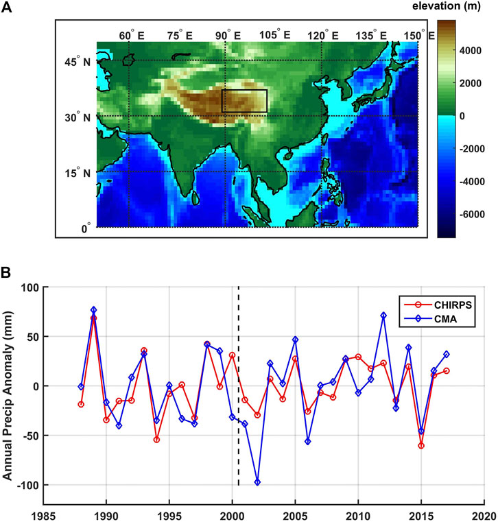
FIGURE 1. (A) The study region of TRHR (black box) as plotted in an elevation map based on ETOPO-5 (Center, 1988) and (B) time series of the spatially averaged precipitation from CHIRPS (red) and CMA (blue) after standardization.

The CHIRPS precipitation is double checked against the station-based precipitation (1988–2017) collected from the China Meteorological Administration (CMA). 55 stations with missing data ratio lower than 20% within the study region are selected and the arithmetically averaged precipitation time series is compared against that from the CHIRPS precipitation. A systematic shift is observed around 2000 for both precipitation though the shift is less significant for the station-based precipitation. While difference in the shifts can be due to non-uniform distribution of the CMA stations, we do not want to diverge into this topic. Instead, the shift is removed by separately standardizing the precipitation over 1981–2000 and 2001–2019. The standardization is done by subtracting the mean and dividing by the standard deviation. The standardized CHIRPS precipitation shows good consistency with the station-based precipitation as shown in Figure 1B, and correlation is 0.67 for 39 samples (p-value < 0.01). The binary TRHR precipitation is used in the multinomial regression model and the two states are defined as: 0 or dry for standardized precipitations smaller than 0 and 1 or wet for standardized precipitations greater than 0.

SST is selected as the primary predictor since it can indicate perturbations in large-scale atmospheric circulations “anchored” in ocean memory (Xie et al., 2009, Xie et al., 2016). Also, the SST field is less spatially heterogeneous compared to that of other common climate variables including geopotential height, vertical velocity of atmosphere (OMEGA) and wind velocities (Peng et al., 2020), which can help improve robustness of the regression models. Monthly SST data is collected from the Hadley Centre Sea Ice and Sea Surface Temperature (HadISST) data set with a spatial resolution of 1° by 1° (Rayner et al., 2003) over Jan 1979–Dec 2019. Only SSTs from the Pacific Ocean and Indian Ocean basins are used to limit our study to regional processes and the basin range is based on the definitions from the National Oceanic and Atmospheric Administration (NOAA) via https://www.nodc.noaa.gov/woce/woce_v3/wocedata_1/woce-uot/summary/bound.htm. Similar positive shifts are observed for most parts of the Pacific Ocean and Indian Ocean as seen in Supplementary Figure S1. To be consistent with the standardization of precipitation, the SSTs are too standardized separately for 1979–2000 and 2001–2019 to remove effects of the trends. This step is to ensure that model skill as measured by the correlation coefficient in the later sections will not be biased by the trends. The only difference here is that standardization of the SSTs is done locally for each grid and uses the monthly climatology means and standard deviations to remove the seasonal cycle.

3 Methods

3.1 The Regularized Regression

Here, we propose a two-step generalized regression model with regularization for dealing with collinearity when developing linear prediction models. The model first reduces dimensionality of the predictors using pooling which is a commonly used method for down-sampling input representations. Then a regularized regression model is fitted using the pooled predictors to estimate real-valued or categorical predictand. A schematic is shown in Figure 2. In the pooling step, a new grid (in green) is defined by some characteristic values (e.g., maximum or median) of the four small grids. The extra step of standardization is to remove the systematic shift in precipitation around 2000 and to rescale precipitation and SSTs (as they have different amplitudes). In this study, we compared model performance using different pooling approaches (i.e., maximum/median/minimum pooling) with a squared window of four grids by four grids.

FIGURE 2

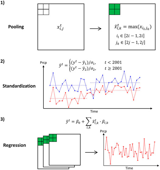
FIGURE 2. A schematic of the proposed the regression model coupling max pooling and elastic net.

The regularized regression is given by Eq. 1 with regression coefficient (β, β₀) (β₀ is the intercept), and it allows flexibility by using different deviance function (Dev) for predictands of different types. For example, the mean squared error (MSE) function is used for estimating the real-valued predictand and the log-likelihood function is used for categorical predictand (Hastie et al., 2009). The deviance function is rescaled by one over the total sample length N. The elastic net regression is adopted here and the regularization term uses a linear combination of the L-1 and L-2 norms of the regression coefficients as shown in Eq. 2.

$(\mathit{\beta },{\beta }_0)=\underset{\beta ,{\beta }_0}{\min }\left(\frac{1}{N}Dev(\mathit{\beta },{\beta }_0)+\lambda P_{\alpha }(\mathit{\beta })\right)(1)$

$P_{\alpha }(\mathit{\beta })=\frac{1-\alpha }{2}{‖\mathit{\beta }‖}_2^2+\alpha {‖\mathit{\beta }‖}_1(2)$

There are two hyperparameters in the model: α and λ. α balances the regularization between the L-1 and L-2 norms of the regression coefficients β and is set to 0.01 for better visualization (Peng et al., 2020). λ is usually decided using a k-fold (e.g., 5-fold) cross validation (CV) (Tibshirani, 1996) and the λ value associated with minimum cross-validated mean squared errors is used (often referred to as the MinMSE λ). However, this procedure can be computationally burdensome since we have to repeat the CV for all lead times. Therefore, a constant λ is firstly determined using the training set data at 0-months lead and is used for all lead times. A preliminary study demonstrates that the significant predictive skill spikes in the testing period are not sensitive over a rather broad range of λs as shown in Supplementary Figure S2. For the true-amplitude predictand, the Pearson’s correlation coefficient (CC) and the Nash–Sutcliffe efficiency (NSE) score are used for model performance evaluation. For the binary predictand, an accuracy score S is defined as given by Eq. 3 where 1 is an indicator function and $\widehat{y}$ is the predicted probability of y being 1 (i.e., wet).

$S=\frac{1}{N}\sum _{i=1}^N\left\{y_i\cdot \mathbf{1}({\widehat{y}}_i\ge 0.5)+(1-y_i)\cdot \mathbf{1}({\widehat{y}}_i<0.5)\right\}(3)$

3.2 Other Regression Models

Performance of the elastic net is compared against some commonly used regression methods in the two-step scheme including the OLS mutil-linear regression (see Hurrell (1996) for details), the EOF regression (see Wakabayashi and Kawamura (2004) for details), and the CCA regression (see Sun and Kim (2016) for details). All regression methods use the same pooled SSTs as the predictors. Though pooling can alleviate the issue of over-fitting, dimensionality of the pooled predictors is still highly non-square (39 years by 1,343 grids). The OLS and CCA regression seek for a linear combination of predictors that maximizes its correlation with the predictand and does not regularize the model complexity. The EOF regression first projects the original predictors onto some “dominant” basis vectors (often referred as EOFs) by decomposing the covariance matrix of the predictors, and then uses the EOFs as the new predictors. It can implicitly regularize the model complexity by using only a few EOFs explaining most variance of the original predictors. The EOF is implemented such that the original (pooled) SSTs are projected onto a set of orthonormal time series which constitute the predictors. It should be noted that it impossible to develop a prediction model this way since we are using data from testing set to construct the basis vectors. Here, the most dominant 50 EOFs accounting for over 88% variance of the original SST data are used in the EOF regression model.

3.3 The Correlation Analysis

A correlation analysis is designed to measure if any correlation patterns between the predictand precipitation and the predictor SSTs persist through time. We propose a new correlation metric L to quantitatively measure persistence of any correlation patterns: for a certain lead time, we first compute lagged correlations between the TRHR precipitation and SSTs at every grid for 1981–2000 and vectorize the correlation map into a column vector denoted by M₁; then this step is repeated for 2001–2019 to compute the column vector M₂; at last, L is defined by computing the correlation coefficients between the vectorized correlation maps M₁ and M₂. L is bounded by a upper limit of 1, which represents the extreme scenario where the correlations between the TRHR precipitation and the SSTs are perfectly consistent before and after 2001 and therefore, a good regression model trained on 1981–2000 should produce significantly high predictive skill on the testing period of 2001–2019. However, L being close to zero does not necessarily mean no predictive skill for regression models since L measures persistence of the global correlations between the TRHR precipitation and the SSTs while the regression model could pick some regional clusters of SSTs that have a persistent correlation with the predictand precipitation. The metric L is used here to estimate how much degradation of performance is resulted from over-fitting by comparing against the testing period predictive skill from the regression models.

4 Results and Discussions

4.1 Comparison of Regression Models

Performance of the regularized regression models in predicting the TRHR precipitation in true amplitudes is examined in this section. The period of 1981–2000 is set as the training period while 2001–2019 is set as the testing period to be consistent with the standardization procedure. Prelim analysis with randomly split data sets demonstrated consistent model skill patterns as shown in Supplementary Figure S3. Since both pooling and regularization are designed for effective dimensionality reduction and thus to avoid over-fitting, we first justify using the extra step of pooling by comparing predictive skill of the regularized regression models with and without pooling. The comparison of testing period correlation coefficients are shown for regression models without pooling and with maximum, median, and minimum pooling in Figure 3. Two spikes are observed at lead times of 13–14 months and 21–24 months. Significant improvement in model skill is shown for lead times of 13–14 months when pooling is used and at the lead time of 13 months, the predictive skill drops to below p-value = 0.1 significance level using non-pooled SSTs. For lead times of 21–24 months, consistent improvement, though less significant, is observed. The improvement could be due to the fact that while there exist some consistent large-scale circulation patterns, the signals may not be fixed to certain grids depending on the spatial resolution and projection coordinate system. Therefore, the model robustness can be improved by including signals of the neighboring grids with pooling. However, though not examined here, one must be careful with choosing the pooling window size since displacement of some circulation patterns can be important indicators of climate anomalies (McGregor et al., 2014; Manatsa et al., 2014) and this information may not be resolved when the pooling window is too large. It should be noted that the λ is re-calibrated for the regression models using non-pooled SSTs. And the statistical significance for the regularized regression is not straightforward to calculate and thus is not reported (Javanmard and Montanari, 2014). The maximum pooling is used in the following analyses.

FIGURE 3

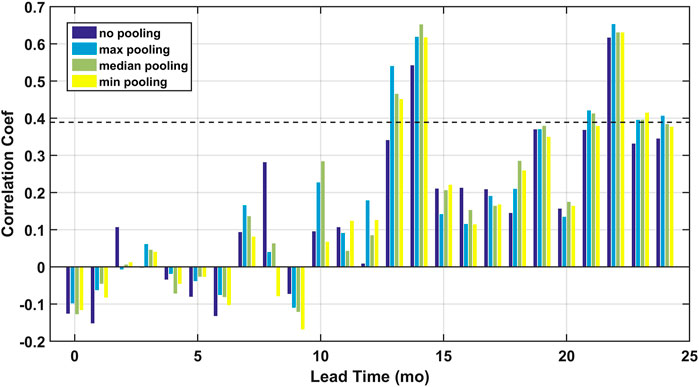
FIGURE 3. Comparison of the predictive skill in the testing period from the elastic net regression models with no pooling (dark blue), maximum pooling (light blue), median pooling (green) and minimum pooling (yellow). The p-value = 0.1 significance level is plotted in the black dashed line.

Model skill for the testing period data as measured by the NSE scores is reported in Figure 4. Consistent patterns are observed as two spikes of NSE scores are found around lead times of 14 and 22 months. However, even at those two lead times, the predictive skill is barely satisfactory. By further looking at comparison between the observed and estimated precipitation, we figured that the elastic net model markedly underestimated the predictand amplitude. However, the extent of shrinking is consistent across the training and testing periods (as shown in Supplementary Figure S4A) and thus, in practice, one could ‘learn’ how much the amplitude is shrunk by looking at the training data and can then rescale testing period estimations. The rescaled estimations show significantly improved NSE scores (NSE = 0.36 for lead time of 14 months and 0.38 for lead time of 22 months (as shown in Supplementary Figure S4B)). A plausible explanation is that the elastic net regression sacrifices accuracy in amplitude estimation for model robustness by selecting only a few predictors and shrinking amplitudes of regression coefficients. This effect is more significant with highly non-square data as in our case since greater regularization must be applied. Therefore, amplitude-based measures such as NSE and the root mean square error (RMSE) may not be applicable for model evaluation. The rescaling method discussed above is not recommended since the model is designed to be biased for more robustness, and in following analyses, the Pearson’s correlation coefficient is used as the primary measure of model skill.

FIGURE 4

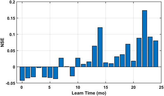
FIGURE 4. Predictive skill for the testing set as a function of lead time reported in the NSE scores.

We then justify using the regularization by comparing predictive skill of the regression with and without regularization. Comparison of the model skill from the elastic net, OLS, EOF, and CCA regression models are shown in Figure 5. Statistically significant positive predictive skill is only observed for the elastic and CCA regressions models. The elastic net models show two spikes of good predictive skill at lead times of 13–14 months and 21–24 months. Statistically significant positive skill is observed for the CCA regression models only at the lead time of 18 months while that of the elastic net regression almost hit the p-value = 0.1 significance level at the lead time of 19 months. Overall, the elastic net regression shows more potential in finding the linear associations between the TRHR precipitation and the SSTs. While statistically significant positive skill are only found at rather long lead times, this does not necessarily mean that there is no connection between the TRHR precipitation and large-scale climate fields at shorter lead times. We are limiting our analysis to only using SSTs from the Pacific and Indian Oceans which is only one sector of the complex large-scale circulations including a wider range of variables like geopotential heights, humidity, vertical velocity of atmosphere (OMEGA) and horizontal winds etc. Furthermore, we are limiting our analysis in the frame of linear models as we compare different types of regression models. Instead of developing accurate forecast models, our intent is to examine how pooling and regularization would improve performance of the linear models at rather low costs. The better performance of elastic net is understandable here since it explicitly regularizes model complexity and provokes sparsity in regression coefficients by using the L-1 norm regularization.

FIGURE 5

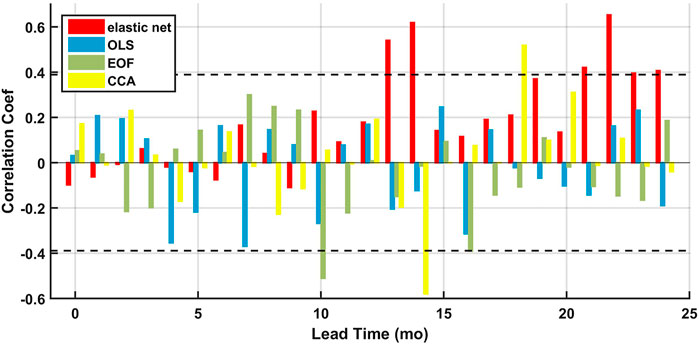
FIGURE 5. Prediction skill for the testing set of 2001–2019 as measured by the correlation coefficients as function of lead times for elastic net (red), OLS (blue), EOF (green), and CCA (yellow). The p-value = 0.1 significance level is plotted in the black dashed lines.

4.2 Source of High Model Skill

A correlation analysis is conducted to measure at a certain lead time, how well a linear model based on the global correlation between the TRHR precipitation and the SSTs can perform. The potential predictive skill is estimated by the new correlation metric L defined earlier as L measures how the time-shifted global correlation patterns persist from 1981 to 2000 (the training period) to 2001–2019 (the testing period). A comparison between L and the predictive skill of the elastic net model at varying lead times is shown in Figure 6. Spikes in L are observed at lead times of 7, 14, 18, and 22 months. Three of the spikes coincide with good predictive skill from the elastic net model (i.e., lead times of 14, 19, and 22 months) while only one of the spike coincide with good skill from other regression models (i.e., lead time of 18 months for the CCA regression model). To estimate how much potential are realized for each model, correlation coefficients between the series of L and model skill from regression models over the lead times of 0–24 months are computed and reported in Table 1. The only statistically significant correlation is found for the elastic net model (0.82 for 25 samples, p-value < 0.01) while rather low correlations are found for other regression models. The results suggest that the OLS, EOF, and CCA regression models do not perform well even when there exist persistent correlations between the predictand precipitation and the SSTs.

FIGURE 6

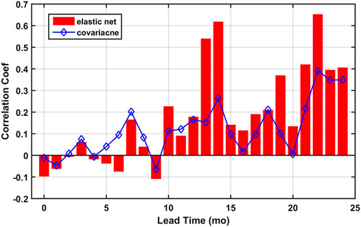
FIGURE 6. Comparison between the predictive skill from the elastic net model (bar) and Ls (blue diamond) at varying lead times. The statistical significance levels are not shown here as we are comparing correlation coefficients calculated using samples of different lengths (19 for the predictive skill and 39 for the Ls).

TABLE 1

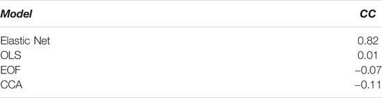
TABLE 1. Correlations between L and prediction skill at varying lead times for different regression models.

Possible explanations are proposed here based on algorithms of the regression methods. For the OLS and CCA regression, the models could be over-fitted to the noisy SST signals for high training skill as both methods decompose the covariance between the predictand precipitation and SSTs to seek a linear combination that either minimizes the MSE (for OLS) or maximizes the correlation (for CCA). Thus, the models are less robust and can perform poorly when evaluated using the testing period samples. As for the EOF regression, the EOF re-constructs the predictors by projecting the global covariance of the SSTs onto some dominant orthonormal basis vectors (EOFs). There are two limiting factors: 1) the assumption of orthogonality may not be appropriate as the new predictors are constructed from the physical variable of SST; 2) any regional persistent correlation patterns between the TRHR precipitation and the SSTs could be lost if they do not make significantly large contribution to the global covariance. Technically, we are not predicting the TRHR precipitation with the EOF regression models since data of the full study period (1981–2019) is used for constructing the new set of predictors (i.e., EOFs).

Interestingly, comparably high predictive skill are observed for the elastic net models at lead times of 14 and 22 months while persistence of the global correlation is much lower at the lead time of 14 months as indicated by L. We specifically looked at the correlation maps between the TRHR precipitation and the SSTs before and after 2000 for the lead times of 14 and 22 months as shown in Figures 7, 8, respectively. For the lead time of 14 months: before 2000, the correlation map features a cluster of positive correlations [180E-210E, 45S-15S] to the east of Australia and an extended band of positive correlations over the mid-north Pacific Ocean [120E-210E, 15N-30N]. Scattered and less significant positive correlations are observed over the northern Indian Ocean and to the west of South America; After 2000, the correlation map is dominated by two major clusters of positive correlations to the east of Australia [180E-210E, 45S-15S] and to the west of South America [260E-280E, 60S-15S] and one major cluster of negative correlations over the southwestern Indian Ocean [30E-60E, 60S-30S]. Less significantly positive correlations are observed over the north-western Pacific which overlaps with the extended band before 2000. For the lead time of 22 months, both correlation maps before and after 2000 are dominated by large clusters of positive correlations over the northern Indian Ocean [60E-90E, 15S-15N] and eastern tropical Pacific Ocean [210E-270E, 15S-0]. The major difference is that clusters of positive correlations over the southern-eastern Pacific and the mid-western Pacific [120E-150E, 15N-30N] get enhanced in correlation amplitude and extended in spatial coverage. A comparison between Figures 7, 8 suggests a higher level of persistence in the global correlation between the predictand precipitation and the SSTs at the lead time of 22 months, which is consistent with the higher value of L in Figure 6. However, a lower value of L does not necessarily mean low predictive skill potential for a linear model as some regional persistent correlation patterns are observed (i.e., the positive correlation cluster to the east of Australia) for the lead time of 14 months. The correlation maps are further compared with the regression coefficient maps in Section 4.3 as we attempt to interpret the high model skill of the elastic net regression.

FIGURE 7

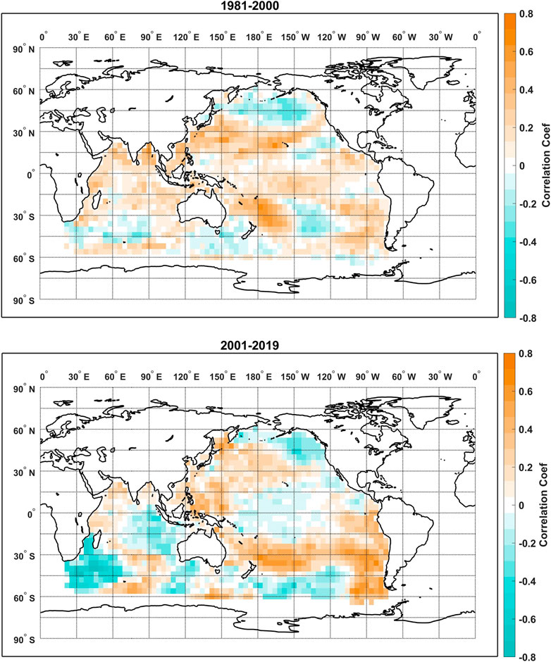
FIGURE 7. Correlation maps between the TRHR precipitation and the SSTs over the training period of 1981–2000 (top) and the testing period of 2001–2019 (bottom) at the lead time of 14 months.

FIGURE 8

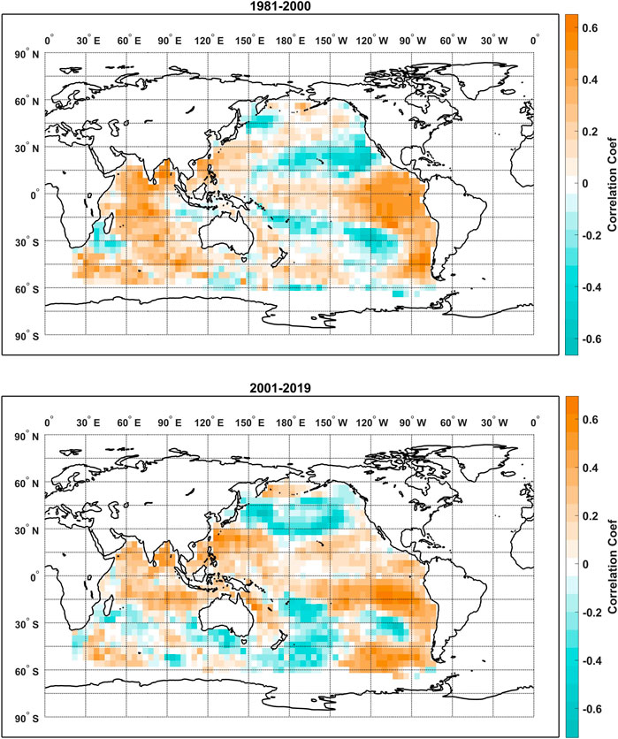
FIGURE 8. Correlation maps between the TRHR precipitation and the SSTs over the training period of 1981–2000 (top) and the testing period of 2001–2019 (bottom) at the lead time of 22 months.

4.3 An Alternative Multinomial Regression Model

In this section, the binary precipitation is predicted using the multinomial regression version (i.e., the elastic net logistic regression) of our model. While new machine learning techniques like the classification and regression tree (CART) can have better model skill in multi-class prediction of climate variables (Choubin et al., 2018; Huang et al., 2021), the elastic net logistic regression is tested to demonstrate flexibility and consistency with altered deviance functions. The multinomial regression may have more use in practical application since amplitudes of the predictand tend to be underestimated because of the regularization (Peng et al., 2020). The logistic regression is implemented by simply replacing the MSE function with the log-likelihood function for Dev (Hastie et al., 2009). Though the logistic regression is a special case of the multinomial regression, the model could be easily generalized for predictand of more than two categories by separately fitting a regularized Poisson regression for each category of which the coefficients are used to estimate the coefficients of the multinomial regression model (Baker, 1994).

To extend the sample size, the leave-one-out cross validation is used (the testing sample size is thus increased from 19 to 39 here). The leave-one-out CV is not used in the previous analysis for predicting real-valued predictand since the Pearson’s correlation coefficient is used for performance evaluation and the leave-one-out CV could result in bias for violating continuity in data. The accuracy as measured by the S score as a function of lead time is shown in Figure 9. A consistent spike of high accuracy (over 70% accuracy) is observed at around lead times of 22 months. While a local maximum of accuracy is observed at the lead time of 14 months, it is not statistically significant. A major reason could be that the S score is not the equivalent measure of the correlation coefficient as we used in Figures 3, 5. A example of high correlation but low S is when the model could well predict the extreme events but performs poorly for the less extreme events.

FIGURE 9

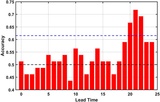
FIGURE 9. Accuracy of predicting the wet-dry state of TRHR precipitation at varying lead times. The base skill (the null model of totally random guess) is plotted in the black dashed line. The one-tailed p-value = 0.1 significance level is estimated using bootstrapping and is plotted in the blue dashed line. The mean accuracy using a totally random guess strategy for 39 samples is collected from 10,000 repeated experiments and the 90th quantile value is used as estimation of the p-value = 0.1 significance level.

Consistency between the regression models using predictand and deviance function of different types is further examined by comparing the maps of the regressions coefficients for lead times of 14 and 22 months as shown in Figures 10, 11, respectively. For the lead time of 14 months, both models feature a major cluster of positive coefficients to the east of Australia while more non-zero coefficients are observed for the logistic regression model over the southeastern Pacific Ocean and the Indian Ocean. As for the lead time of 22 months, both maps are dominated by the large cluster of positive coefficients over the eastern tropical Pacific Ocean. While positive coefficients are observed over the northern Indian Ocean for both models, the coefficients are more sparsely distributed for the model using the true-amplitude predictand. More non-zero coefficients are found for the logistic regression model at both lead times, which could be due to a less optimal regularization as we only did the cross validation on a relatively sparse sequence of λs with a lead time of 0 months. But overall, the major clusters of non-zero regression coefficients are consistent across the models. And this is also confirmed by the results that statistically significant correlations are found between the vectorized coefficient maps of the two models. The correlation coefficients are 0.45 for the lead time of 14 months and 0.44 for the lead time of 22 months (1,343 samples) and are 0.35 for the lead time of 14 months (327 samples) and 0.40 for the lead time of 22 months (359 samples) when only the non-zero coefficients are considered.

FIGURE 10

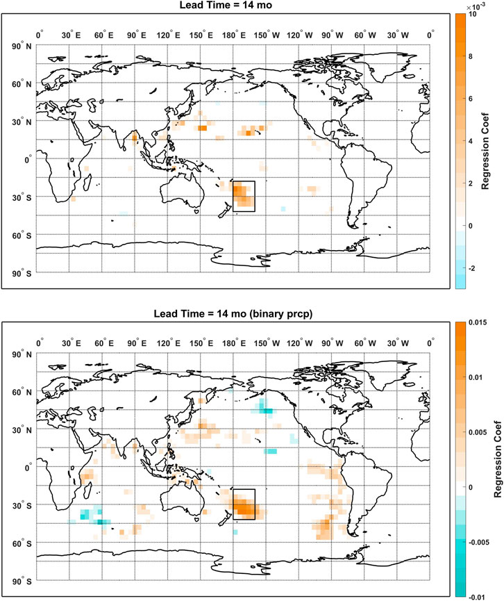
FIGURE 10. Maps of regression coefficients from the elastic net models using true-amplitude (top) and binary (bottom) predictand precipitation at the lead time of 14 months.

FIGURE 11

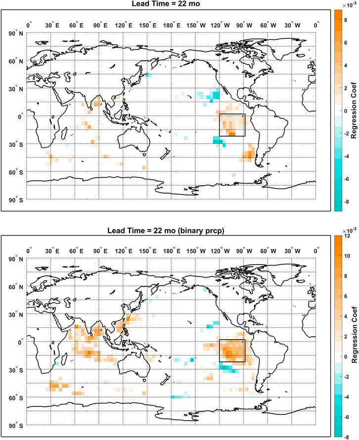
FIGURE 11. Maps of regression coefficients from the elastic net models using true-amplitude (top) and binary (bottom) predictand precipitation at the lead time of 22 months.

The comparably high predictive skill at the lead time of 14 months is easy to interpret if we compare the coefficient maps from Figures 10, 11 to the correlation maps from Figures 7, 8. While less persistence is observed for the global correlation at the lead time of 14 months, the elastic net model managed to select the regional persistent cluster of positive correlations to the east of Australia. At last, two SST indices are defined based on the consistent patterns from the two regression models: the SST index 1 is defined by the mean SST over the domain of [180°W-160°W, 42°S-18°S]; the SST index 2 is defined by the mean SST over the domain of [120°W-88°W, 22°S-2°N]. Lagged correlations between the TRHR precipitation and the SST indices calculated using the non-pooled and pooled SSTs are plotted in Figure 12. Statistically significant positive correlations are observed at the corresponding lead times and consistent results are shown for non-pooled and pooled SSTs. The results suggest that the proposed framework managed to select certain regional SSTs that are consistently correlated with the predictand precipitation and demonstrated good interpretability. While correlation does not necessarily imply causation, the elastic net regression models show good potential here in guiding further research with its highly interpretable and flexible models.

FIGURE 12

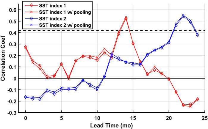
FIGURE 12. Lagged correlations between the TRHR precipitation and the SST indices. The p-value = 0.01 significance level is plotted in the black dashed line.

5 Conclusion

In this paper, we tested a generalized regression model with regularization coupled with pooling in predicting the TRHR wet-season precipitation at lead times of 0–24 months using the Pacific and Indian Ocean SSTs. The regression is first tested using the true-amplitude predictand and is compared against some widely-used regression models including the OLS multi-linear regression, the EOF regression and the CCA regression. Significantly good predictive skill are observed using the elastic net regression models for certain long lead times which are further examined using a correlation analysis. The results suggest that the elastic net regression achieves good performance in identifying and using the persistent correlation patterns while the other three regression models show relatively poor performance. Low model skill at shorter lead times can be due to that only SST is used as the predictor while teleconnection signals can propagate through other climate fields chronologically. A multinomial elastic net regression model is then used to demonstrate flexibility and consistency of the proposed framework. Consistent model skill and regression coefficient maps are observed even when predictand and deviance functions of different types are used. By comparing the correlation analysis and the regression coefficient maps, we found that the elastic net model managed to select regional persistent correlation patterns as the contributing predictors while the other widely-used regression models are based on the global covariance either between the predictand and the predictors or within the predictors (and thus are vulnerable to over-fitting). At last, two SST indices are defined based on the major clusters of non-zeros coefficients from the elastic net models and are found to be significantly correlated to the TRHR precipitation at the corresponding lead times. Overall, the proposed framework demonstrates good interpretability in identifying covariates with high predictive skill and the potential in guiding further investigation using more complex, nonlinear statistical models or physically based modeling experiments.

Data Availability Statement

The original contributions presented in the study are included in the article/Supplementary Material. The codes are processed data can be found via https://github.com/cruiseryy/TRHR_elasticnet_pooling and further inquiries can be directed to the corresponding author.

Author Contributions

The idea originated from a discussion among the three authors. XP and JA designed the study and XP carried out the experiment, and wrote the article. JA oversaw the entire project. JA and TL offered technical advice during the experiment and provided inputs to the article writing. All authors contributed to the article and approved the submitted version.

Funding

The Cornell authors were supported by the Cornell China Center under the project of “Food-Energy-Water Security in the Three-Rivers Headwater Region: Integrating Science, Data and Decision Tools to Manage Under a Changing Climate and Development Pressure”. The Tsinghua author was supported by the National Key Research and Development Program of China (No. 2016YFE0201900), and the Research Fund of the State Key Laboratory of Hydroscience and Engineering, Tsinghua University (No. 2017-KY-04).

Conflict of Interest

The authors declare that the research was conducted in the absence of any commercial or financial relationships that could be construed as a potential conflict of interest.

Publisher’s Note

All claims expressed in this article are solely those of the authors and do not necessarily represent those of their affiliated organizations, or those of the publisher, the editors and the reviewers. Any product that may be evaluated in this article, or claim that may be made by its manufacturer, is not guaranteed or endorsed by the publisher.

Acknowledgments

The rainfall data were collected from the CHIRPS (http://chg.geog.ucsb.edu/data/chirps/) and the China Meteorological Administration (CMA). The SST data were collected from the HadISST dataset (https://www.metoffice.gov.uk/hadobs/hadisst/). We thank the two reviewers for their insightful comments.

Supplementary Material

The Supplementary Material for this article can be found online at: https://www.frontiersin.org/articles/10.3389/feart.2021.724599/full#supplementary-material

References

Akaike, H. (1998). “Information Theory and an Extension of the Maximum Likelihood Principle,” in Selected Papers of Hirotugu Akaike (New York: Springer), 199–213. doi:10.1007/978-1-4612-1694-0_15

CrossRef Full Text | Google Scholar

Ali, M., Deo, R. C., Maraseni, T., and Downs, N. J. (2019). Improving Spi-Derived Drought Forecasts Incorporating Synoptic-Scale Climate Indices in Multi-phase Multivariate Empirical Mode Decomposition Model Hybridized with Simulated Annealing and Kernel ridge Regression Algorithms. J. Hydrol. 576, 164–184. doi:10.1016/j.jhydrol.2019.06.032

CrossRef Full Text | Google Scholar

Baker, S. G. (1994). The Multinomial-Poisson Transformation. The Statistician. 43, 495–504. doi:10.2307/2348134

CrossRef Full Text | Google Scholar

Benn, D. I., and Owen, L. A. (1998). The Role of the Indian Summer Monsoon and the Mid-latitude Westerlies in Himalayan Glaciation: Review and Speculative Discussion. J. Geol. Soc. 155, 353–363. doi:10.1144/gsjgs.155.2.0353

CrossRef Full Text | Google Scholar

Block, P. (2011). Tailoring Seasonal Climate Forecasts for Hydropower Operations. Hydrol. Earth Syst. Sci. 15, 1355–1368. doi:10.5194/hess-15-1355-2011

CrossRef Full Text | Google Scholar

Bueso, D., Piles, M., and Camps-Valls, G. (2020). Nonlinear Pca for Spatio-Temporal Analysis of Earth Observation Data. IEEE Trans. Geosci. Remote. Sens. 58, 5752–5763. doi:10.1109/tgrs.2020.2969813

CrossRef Full Text | Google Scholar

Carpenter, T. M., and Georgakakos, K. P. (2001). Assessment of folsom lake Response to Historical and Potential Future Climate Scenarios: 1. Forecasting. J. Hydrol. 249, 148–175. doi:10.1016/s0022-1694(01)00417-6

CrossRef Full Text | Google Scholar

Carvalho, D. V., Pereira, E. M., and Cardoso, J. S. (2019). Machine Learning Interpretability: A Survey on Methods and Metrics. Electronics 8, 832. doi:10.3390/electronics8080832

CrossRef Full Text | Google Scholar

Center, N. G. D. (1988). Data From: Etopo-5 Bathymetry/topography Data

Google Scholar

Chen, C., Li, T., Sivakumar, B., Li, J., and Wang, G. (2020). Attribution of Growing Season Vegetation Activity to Climate Change and Human Activities in the Three-River Headwaters Region, china. J. Hydroinformatics 22, 186–204. doi:10.2166/hydro.2019.003

CrossRef Full Text | Google Scholar

Choubin, B., Zehtabian, G., Azareh, A., Rafiei-Sardooi, E., Sajedi-Hosseini, F., and Kişi, Ö. (2018). Precipitation Forecasting Using Classification and Regression Trees (Cart) Model: a Comparative Study of Different Approaches. Environ. earth Sci. 77, 1–13. doi:10.1007/s12665-018-7498-z

CrossRef Full Text | Google Scholar

DelSole, T., and Banerjee, A. (2017). Statistical Seasonal Prediction Based on Regularized Regression. J. Clim. 30, 1345–1361. doi:10.1175/jcli-d-16-0249.1

CrossRef Full Text | Google Scholar

Devineni, N., and Sankarasubramanian, A. (2010). Improving the Prediction of winter Precipitation and Temperature over the continental united states: Role of the Enso State in Developing Multimodel Combinations. Monthly Weather Rev. 138, 2447–2468. doi:10.1175/2009mwr3112.1

CrossRef Full Text | Google Scholar

Dong, Y., Zhai, J., Zhao, Y., Li, H., Wang, Q., Jiang, S., et al. (2020). Teleconnection Patterns of Precipitation in the Three-River Headwaters Region, china. Environ. Res. Lett. 15, 104050. doi:10.1088/1748-9326/aba8c0

CrossRef Full Text | Google Scholar

Enfield, D. B., Mestas-Nuñez, A. M., Mayer, D. A., and Cid-Serrano, L. (1999). How Ubiquitous Is the Dipole Relationship in Tropical atlantic Sea Surface Temperatures? J. Geophys. Res. 104, 7841–7848. doi:10.1029/1998jc900109

CrossRef Full Text | Google Scholar

Fan, Y. R., Huang, W., Huang, G. H., Li, Z., Li, Y. P., Wang, X. Q., et al. (2015). A Stepwise-Cluster Forecasting Approach for Monthly Streamflows Based on Climate Teleconnections. Stoch Environ. Res. Risk Assess. 29, 1557–1569. doi:10.1007/s00477-015-1048-y

CrossRef Full Text | Google Scholar

Feng, L., and Zhou, T. (2012). Water Vapor Transport for Summer Precipitation over the Tibetan Plateau: Multidata Set Analysis. J. Geophys. Res. Atmospheres. 117, 1–21. doi:10.1029/2011jd017012

CrossRef Full Text | Google Scholar

Funk, C., Peterson, P., Landsfeld, M., Pedreros, D., Verdin, J., Shukla, S., et al. (2015). The Climate Hazards Infrared Precipitation with Stations-a New Environmental Record for Monitoring Extremes. Sci. Data. 2. doi:10.1038/sdata.2015.66

CrossRef Full Text | Google Scholar

Gilpin, L. H., Bau, D., Yuan, B. Z., Bajwa, A., Specter, M., and Kagal, L. (2018). “Explaining Explanations: An Overview of Interpretability of Machine Learning,” in 2018 IEEE 5th International Conference on data science and advanced analytics (DSAA), Turin, Italy, October 1–4, 2018 ((IEEE)), 80–89. doi:10.1109/dsaa.2018.00018

CrossRef Full Text | Google Scholar

Goddard, L., Mason, S. J., Zebiak, S. E., Ropelewski, C. F., Basher, R., and Cane, M. A. (2001). Current Approaches to Seasonal to Interannual Climate Predictions. Int. J. Climatol. 21, 1111–1152. doi:10.1002/joc.636

CrossRef Full Text | Google Scholar

Ham, Y.-G., Kim, J.-H., and Luo, J.-J. (2019). Deep Learning for Multi-Year Enso Forecasts. Nature 573, 568–572. doi:10.1038/s41586-019-1559-7

PubMed Abstract | CrossRef Full Text | Google Scholar

Hansen, J. W., Mason, S. J., Sun, L., and Tall, A. (2011). Review of Seasonal Climate Forecasting for Agriculture in Sub-saharan Africa. Ex. Agric. 47, 205–240. doi:10.1017/s0014479710000876

CrossRef Full Text | Google Scholar

Hastie, T., Tibshirani, R., and Friedman, J. (2009). The Elements of Statistical Learning: Data Mining, Inference, and Prediction. New York: Springer Science & Business Media.

Hoerl, A. E., and Kennard, R. W. (1970). Ridge Regression: Biased Estimation for Nonorthogonal Problems. Technometrics 12, 55–67. doi:10.1080/00401706.1970.10488634

CrossRef Full Text | Google Scholar

Huang, L., Kang, J., Wan, M., Fang, L., Zhang, C., and Zeng, Z. (2021). Solar Radiation Prediction Using Different Machine Learning Algorithms and Implications for Extreme Climate Events. Front. Earth Sci. 9, 202. doi:10.3389/feart.2021.596860

CrossRef Full Text | Google Scholar

Hurrell, J. W. (1996). Influence of Variations in Extratropical Wintertime Teleconnections on Northern Hemisphere Temperature. Geophys. Res. Lett. 23, 665–668. doi:10.1029/96gl00459

CrossRef Full Text | Google Scholar

Javanmard, A., and Montanari, A. (2014). Confidence Intervals and Hypothesis Testing for High-Dimensional Regression. J. Machine Learn. Res. 15, 2869–2909. doi:10.5555/2627435.2697057

Google Scholar

Kalchbrenner, N., Grefenstette, E., and Blunsom, P. (2014). A Convolutional Neural Network for Modelling Sentences. arXiv. preprint arXiv:1404.2188.

Kharin, V. V., and Zwiers, F. W. (2002). Climate Predictions with Multimodel Ensembles. J. Clim. 15, 793–799. doi:10.1175/1520-0442(2002)015<0793:cpwme>2.0.co;2

CrossRef Full Text | Google Scholar

Kim, J., Oh, H.-S., Lim, Y., and Kang, H.-S. (2017). Seasonal Precipitation Prediction via Data-Adaptive Principal Component Regression. Int. J. Climatol. 37, 75–86. doi:10.1002/joc.4979

CrossRef Full Text | Google Scholar

Krishnamurti, T. N., Kishtawal, C. M., LaRow, T. E., Bachiochi, D. R., Zhang, Z., Williford, C. E., et al. (1999). Improved Weather and Seasonal Climate Forecasts from Multimodel Superensemble. Science 285, 1548–1550. doi:10.1126/science.285.5433.1548

PubMed Abstract | CrossRef Full Text | Google Scholar

Lemos, M. C., Finan, T. J., Fox, R. W., Nelson, D. R., and Tucker, J. (2002). The Use of Seasonal Climate Forecasting in Policymaking: Lessons from Northeast brazil. Clim. Change. 55, 479–507. doi:10.1023/a:1020785826029

CrossRef Full Text | Google Scholar

Li, J., Pollinger, F., and Paeth, H. (2020). Comparing the Lasso Predictor-Selection and Regression Method with Classical Approaches of Precipitation Bias Adjustment in Decadal Climate Predictions. Monthly Weather Rev. 148, 4339–4351. doi:10.1175/mwr-d-19-0302.1

CrossRef Full Text | Google Scholar

Liu, P. (2015). A Survey of Remote-Sensing Big Data. Front. Environ. Sci. 3, 45. doi:10.3389/fenvs.2015.00045

CrossRef Full Text | Google Scholar

Manatsa, D., Morioka, Y., Behera, S. K., Matarira, C. H., and Yamagata, T. (2014). Impact of Mascarene High Variability on the East African 'short rains'. Clim. Dyn. 42, 1259–1274. doi:10.1007/s00382-013-1848-z

CrossRef Full Text | Google Scholar

Mantua, N. J., Hare, S. R., Zhang, Y., Wallace, J. M., and Francis, R. C. (1997). A pacific Interdecadal Climate Oscillation with Impacts on salmon Production. Bull. Amer. Meteorol. Soc. 78, 1069–1079. doi:10.1175/1520-0477(1997)078<1069:apicow>2.0.co;2

CrossRef Full Text | Google Scholar

Matsui, H., and Konishi, S. (2011). Variable Selection for Functional Regression Models via the Regularization. Comput. Stat. Data Anal. 55, 3304–3310. doi:10.1016/j.csda.2011.06.016

CrossRef Full Text | Google Scholar

McGregor, S., Timmermann, A., Stuecker, M. F., England, M. H., Merrifield, M., Jin, F.-F., et al. (2014). Recent walker Circulation Strengthening and pacific Cooling Amplified by atlantic Warming. Nat. Clim Change. 4, 888–892. doi:10.1038/nclimate2330

CrossRef Full Text | Google Scholar

Mekanik, F., Imteaz, M. A., Gato-Trinidad, S., and Elmahdi, A. (2013). Multiple Regression and Artificial Neural Network for Long-Term Rainfall Forecasting Using Large Scale Climate Modes. J. Hydrol. 503, 11–21. doi:10.1016/j.jhydrol.2013.08.035

CrossRef Full Text | Google Scholar

Menemenlis, D., Fukumori, I., and Lee, T. (2005). Using Green's Functions to Calibrate an Ocean General Circulation Model. Monthly weather Rev. 133, 1224–1240. doi:10.1175/mwr2912.1

CrossRef Full Text | Google Scholar

Mo, K. C. (2003). Ensemble Canonical Correlation Prediction of Surface Temperature over the united states. J. Clim. 16, 1665–1683. doi:10.1175/1520-0442(2003)016<1665:eccpos>2.0.co;2

CrossRef Full Text | Google Scholar

Mudelsee, M. (2000). Ramp Function Regression: a Tool for Quantifying Climate Transitions. Comput. Geosciences. 26, 293–307. doi:10.1016/s0098-3004(99)00141-7

CrossRef Full Text | Google Scholar

Peng, X., Steinschneider, S., and Albertson, J. (2020). Investigating Long-Range Seasonal Predictability of East African Short rains: Influence of the Mascarene High on the Indian Ocean walker Cell. J. Appl. Meteorology Climatology. 59, 1077–1090. doi:10.1175/jamc-d-19-0109.1

CrossRef Full Text | Google Scholar

Rasmusson, E. M., and Carpenter, T. H. (1982). Variations in Tropical Sea Surface Temperature and Surface Wind Fields Associated with the Southern Oscillation/El Niño. Mon. Wea. Rev. 110, 354–384. doi:10.1175/1520-0493(1982)110<0354:vitsst>2.0.co;2

CrossRef Full Text | Google Scholar

Rayner, N., Parker, D. E., Horton, E., Folland, C. K., Alexander, L. V., Rowell, D., et al. (2003). Global Analyses of Sea Surface Temperature, Sea Ice, and Night marine Air Temperature since the Late Nineteenth century. J. Geophys. Res. Atmospheres. 108. doi:10.1029/2002jd002670

CrossRef Full Text | Google Scholar

Reichstein, M., Camps-Valls, G., Stevens, B., Jung, M., Denzler, J., Carvalhais, N., et al. (2019). Deep Learning and Process Understanding for Data-Driven Earth System Science. Nature 566, 195–204. doi:10.1038/s41586-019-0912-1

PubMed Abstract | CrossRef Full Text | Google Scholar

Rust, H. W., Richling, A., Bissolli, P., and Ulbrich, U. (2015). Linking Teleconnection Patterns to European Temperature: a Multiple Linear Regression Model. Meteorol. Z. 24, 411–423. doi:10.1127/metz/2015/0642

CrossRef Full Text | Google Scholar

Sahastrabuddhe, R., and Ghosh, S. (2021). Does Statistical Model Perform at Par with Computationally Expensive General Circulation Model for Decadal Prediction? Environ. Res. Lett. 16, 064028. doi:10.1088/1748-9326/abfeed

CrossRef Full Text | Google Scholar

Schepen, A., Zhao, T., Wang, Q. J., and Robertson, D. E. (2018). A Bayesian Modelling Method for post-processing Daily Sub-seasonal to Seasonal Rainfall Forecasts from Global Climate Models and Evaluation for 12 Australian Catchments. Hydrol. Earth Syst. Sci. 22, 1615–1628. doi:10.5194/hess-22-1615-2018

CrossRef Full Text | Google Scholar

Schoof, J. T., and Pryor, S. C. (2001). Downscaling Temperature and Precipitation: A Comparison of Regression-Based Methods and Artificial Neural Networks. Int. J. Climatol. 21, 773–790. doi:10.1002/joc.655

CrossRef Full Text | Google Scholar

Schwarz, G. (1978). Index of Authors. J. Hyg. 80, 461–464. doi:10.1017/s0022172400024931

CrossRef Full Text | Google Scholar

Shaman, J., and Tziperman, E. (2005). The Effect of Enso on Tibetan Plateau Snow Depth: A Stationary Wave Teleconnection Mechanism and Implications for the South Asian Monsoons. J. Clim. 18, 2067–2079. doi:10.1175/jcli3391.1

CrossRef Full Text | Google Scholar

Soleh, A. M., Wigena, A. H., Djuraidah, A., and Saefuddin, A. (2015). Statistical Downscaling to Predict Monthly Rainfall Using Linear Regression with L_1 Regularization (LASSO). ams 9, 5361–5369. doi:10.12988/ams.2015.56434

CrossRef Full Text | Google Scholar

Solow, A. R. (1987). Testing for Climate Change: An Application of the Two-phase Regression Model. J. Clim. Appl. Meteorol. 26, 1401–1405. doi:10.1175/1520-0450(1987)026<1401:tfccaa>2.0.co;2

CrossRef Full Text | Google Scholar

Stevens, A., Willett, R., Mamalakis, A., Foufoula-Georgiou, E., Tejedor, A., Randerson, J. T., et al. (2021). Graph-Guided Regularized Regression of Pacific Ocean Climate Variables to Increase Predictive Skill of Southwestern U.S. Winter Precipitation. J. Clim. 34, 737–754. doi:10.1175/jcli-d-20-0079.1

CrossRef Full Text | Google Scholar

Sun, M., and Kim, G. (2016). Quantitative Monthly Precipitation Forecasting Using Cyclostationary Empirical Orthogonal Function and Canonical Correlation Analysis. J. Hydrol. Eng. 21, 04015045. doi:10.1061/(asce)he.1943-5584.0001244

CrossRef Full Text | Google Scholar

Tan, X., and Shao, D. (2017). Precipitation Trends and Teleconnections Identified Using Quantile Regressions over Xinjiang, china. Int. J. Climatol. 37, 1510–1525. doi:10.1002/joc.4794

CrossRef Full Text | Google Scholar

Thornthwaite, C. W. (1948). An Approach toward a Rational Classification of Climate. Geographical Rev. 38, 55–94. doi:10.2307/210739

CrossRef Full Text | Google Scholar

Tibshirani, R. (1996). Regression Shrinkage and Selection via the Lasso. J. R. Stat. Soc. Ser. B (Methodological) 58, 267–288. doi:10.1111/j.2517-6161.1996.tb02080.x

CrossRef Full Text | Google Scholar

Trenberth, K. E., and Stepaniak, D. P. (2001). Indices of El Niño Evolution. J. Clim. 14, 1697–1701. doi:10.1175/1520-0442(2001)014<1697:lioeno>2.0.co;2

CrossRef Full Text | Google Scholar

Trenberth, K. E. (1997). The Definition of El Niño. Bull. Amer. Meteorol. Soc. 78, 2771–2777. doi:10.1175/1520-0477(1997)078<2771:tdoeno>2.0.co;2

CrossRef Full Text | Google Scholar

Van Oldenborgh, G. J., and Burgers, G. (2005). Searching for Decadal Variations in Enso Precipitation Teleconnections. Geophys. Res. Lett. 32. doi:10.1029/2005gl023110

CrossRef Full Text | Google Scholar

Verdin, J., Funk, C., Senay, G., and Choularton, R. (2005). Climate Science and Famine Early Warning. Phil. Trans. R. Soc. B. 360, 2155–2168. doi:10.1098/rstb.2005.1754

PubMed Abstract | CrossRef Full Text | Google Scholar

Von Storch, H., and Zwiers, F. W. (2001). Statistical Analysis in Climate Research. Cambridge University Press.

Wakabayashi, S., and Kawamura, R. (2004). NOTES and CORRESPONDENCE; Extraction of Major Teleconnection Patterns Possibly Associated with the Anomalous Summer Climate in Japan. J. Meteorol. Soc. Jpn. 82, 1577–1588. doi:10.2151/jmsj.82.1577

CrossRef Full Text | Google Scholar

Wilhite, D. A., and Svoboda, M. D. (2000). Drought Early Warning Systems in the Context of Drought Preparedness and Mitigation, in Early Warning Systems for Drought Preparedness and Drought Management. (Geneva: World Meteorological Organization), 1–21.

Google Scholar

Worland, S. C., Steinschneider, S., Asquith, W., Knight, R., and Wieczorek, M. (2019). Prediction and Inference of Flow Duration Curves Using Multioutput Neural Networks. Water Resour. Res. 55, 6850–6868. doi:10.1029/2018wr024463

CrossRef Full Text | Google Scholar

Xie, S.-P., Hu, K., Hafner, J., Tokinaga, H., Du, Y., Huang, G., et al. (2009). Indian Ocean Capacitor Effect on Indo-Western Pacific Climate during the Summer Following El Niño. J. Clim. 22, 730–747. doi:10.1175/2008jcli2544.1

CrossRef Full Text | Google Scholar

Xie, S.-P., Kosaka, Y., Du, Y., Hu, K., Chowdary, J. S., and Huang, G. (2016). Indo-western pacific Ocean Capacitor and Coherent Climate Anomalies in post-enso Summer: A Review. Adv. Atmos. Sci. 33, 411–432. doi:10.1007/s00376-015-5192-6

CrossRef Full Text | Google Scholar

Yang, X., and DelSole, T. (2012). Systematic Comparison of Enso Teleconnection Patterns between Models and Observations. J. Clim. 25, 425–446. doi:10.1175/jcli-d-11-00175.1

CrossRef Full Text | Google Scholar

Yu, D., Wang, H., Chen, P., and Wei, Z. (2014). “Mixed Pooling for Convolutional Neural Networks,” in International conference on rough sets and knowledge technology. Springer, 364–375. doi:10.1007/978-3-319-11740-9_34

CrossRef Full Text | Google Scholar

Zeiler, M. D., and Fergus, R. (2013). Stochastic Pooling for Regularization of Deep Convolutional Neural Networks. arXi. preprint arXiv:1301.3557.

Zhang, S., Gan, T. Y., and Bush, A. B. G. (2020). Variability of Arctic Sea Ice Based on Quantile Regression and the Teleconnection with Large-Scale Climate Patterns. J. Clim. 33, 4009–4025. doi:10.1175/jcli-d-19-0375.1

CrossRef Full Text | Google Scholar

Zhang, Y., Huang, W., and Zhong, D. (2019). Major Moisture Pathways and Their Importance to Rainy Season Precipitation over the Sanjiangyuan Region of the Tibetan Plateau. J. Clim. 32, 6837–6857. doi:10.1175/jcli-d-19-0196.1

CrossRef Full Text | Google Scholar

Zhang, Y., Wallace, J. M., and Battisti, D. S. (1997). ENSO-like Interdecadal Variability: 1900-93. J. Clim. 10, 1004–1020. doi:10.1175/1520-0442(1997)010<1004:eliv>2.0.co;2

CrossRef Full Text | Google Scholar

Zhao, Y., Xu, X., Liao, L., Wang, Y., Gu, X., Qin, R., et al. (2019). The Severity of Drought and Precipitation Prediction in the Eastern Fringe of the Tibetan Plateau. Theor. Appl. Climatol. 137, 141–152. doi:10.1007/s00704-018-2564-8

CrossRef Full Text | Google Scholar

Zou, H., and Hastie, T. (2005). Regularization and Variable Selection via the Elastic Net. J. R. Stat. Soc B. 67, 301–320. doi:10.1111/j.1467-9868.2005.00503.x

CrossRef Full Text | Google Scholar