Climatic and Morphometric Explanatory Variables of Glacier Changes in the Andes (8–55°S): New Insights From Machine Learning Approaches

Caro, Alexis; Condom, Thomas; Rabatel, Antoine

doi:10.3389/feart.2021.713011

ORIGINAL RESEARCH article

Front. Earth Sci., 23 December 2021

Sec. Cryospheric Sciences

Volume 9 - 2021 | https://doi.org/10.3389/feart.2021.713011

This article is part of the Research Topic Glaciation and Climate Change in the Andean Cordillera View all 17 articles

Climatic and Morphometric Explanatory Variables of Glacier Changes in the Andes (8–55°S): New Insights From Machine Learning Approaches

Alexis Caro*

Thomas Condom

Antoine Rabatel

Univ. Grenoble Alpes, CNRS, IRD, Grenoble-INP, Institut des Géosciences de l’Environnement, Grenoble, France

Over the last decades, glaciers across the Andes have been strongly affected by a loss of mass and surface areas. This increases risks of water scarcity for the Andean population and ecosystems. However, the factors controlling glacier changes in terms of surface area and mass loss remain poorly documented at watershed scale across the Andes. Using machine learning methods (Least Absolute Shrinkage and Selection Operator, known as LASSO), we explored climatic and morphometric variables that explain the spatial variance of glacier surface area variations in 35 watersheds (1980–2019), and of glacier mass balances in 110 watersheds (2000–2018), with data from 2,500 to 21,000 glaciers, respectively, distributed between 8 and 55°S in the Andes. Based on these results and by applying the Partitioning Around Medoids (PAM) algorithm we identified new glacier clusters. Overall, spatial variability of climatic variables presents a higher explanatory power than morphometric variables with regards to spatial variance of glacier changes. Specifically, the spatial variability of precipitation dominates spatial variance of glacier changes from the Outer Tropics to the Dry Andes (8–37°S) explaining between 49 and 93% of variances, whereas across the Wet Andes (40–55°S) the spatial variability of temperature is the most important climatic variable and explains between 29 and 73% of glacier changes spatial variance. However, morphometric variables such as glacier surface area show a high explanatory power for spatial variance of glacier mass loss in some watersheds (e.g., Achacachi with r² = 0.6 in the Outer Tropics, Río del Carmen with r² = 0.7 in the Dry Andes). Then, we identified a new spatial framework for hydro-glaciological analysis composed of 12 glaciological zones, derived from a clustering analysis, which includes 274 watersheds containing 32,000 glaciers. These new zones better take into account different seasonal climate and morphometric characteristics of glacier diversity. Our study shows that the exploration of variables that control glacier changes, as well as the new glaciological zones calculated based on these variables, would be very useful for analyzing hydro-glaciological modelling results across the Andes (8–55°S).

1 Introduction

The Andes contain the largest concentration of ice in the southern hemisphere outside the Antarctic and its periphery (RGI Consortium, 2017). Andean glaciers have been affected by an almost continuous negative mass balance and consecutive shrinkage since the middle of the 20th century (Rabatel et al., 2013; Zemp et al., 2019). Despite considerable efforts in recent years regarding quantifications of glacier changes (e.g., Meier et al., 2018; Braun et al., 2019; Dussaillant et al., 2019; Seehaus et al., 2019, 2020), there is still much to investigate in order to analyze the controlling factors of these changes and to determine the hydrological significance of this glacier surface and mass loss on fresh water resources (e.g., Vuille et al., 2018; Masiokas et al., 2020). A better understanding of glacier changes across the Andes could contribute to anticipate and mitigate the related consequences and hazards at watershed scale, for instance in terms of water supply for roughly 45% of the population in Andean countries (Devenish and Gianella, 2012) and for ecosystems (Dangles et al., 2017; Zimmer et al., 2018; Cauvy-Fraunié & Dangles, 2019), primarily during the dry season (Mark et al., 2005; Baraer et al., 2012; Soruco et al., 2015; Guido et al., 2016; Ayala et al., 2020).

Glaciological studies carried out on a limited number of glaciers in the Outer Tropics (8–17°S) have underlined that atmospheric warming is an important control on the current glacier change mainly through the precipitation phases and consecutive albedo effect (Favier et al., 2004; Rabatel et al., 2013). The surface area and elevation of glaciers are morphometric variables that have also been identified to modulate the magnitude of glacier mass loss (e.g., Rabatel et al., 2006, 2013; Soruco et al., 2009). In the Southern Andes (17–55°S), studies focusing on long-term behavior of glaciers (i.e., since the mid-20th century) highlight a high correlation between precipitation and glacier mass balance in the Dry Andes (Rabatel et al., 2011; Masiokas et al., 2016; Kinnard et al., 2020), and with temperature in the Wet Andes (Masiokas et al., 2015; Abdel Jaber et al., 2019; Falaschi et al., 2019). These variables, primarily temperature and precipitation, have been widely used across the Andes to simulate glacier changes and related hydrological contribution through conceptual and physically-based hydro-glaciological models from a local scale to the scale of the Andes (Sicart et al., 2008; Ragettli and Pellicciotti, 2012; Huss and Hock, 2015, 2018; Soruco et al., 2015; Ayala et al., 2016, 2020; Bravo et al., 2017; Mernild et al., 2018; Burger et al., 2019; Shaw et al., 2020).

However, these studies did not quantified the relevance of morphometric variables to estimate glacier changes such as elevation and aspect, or glacier surface area and slope; these variables have already been significantly correlated to glacier changes in studies either dedicated to the Tropical and Southern Andes (e.g., Soruco et al., 2009; Rabatel et al., 2011) or in other mountain ranges (e.g., Rabatel et al., 2016; Brun et al., 2019; Bolibar et al., 2020; Davaze et al., 2020). In addition, simulations of glacier changes are traditionally conducted using geodetic mass balance products and few in situ glacier measurements available for calibration/validation purposes. However, glacier surface area changes are not frequently considered in hydro-glaciological simulations (e.g., Ayala et al., 2020; Baraer et al., 2012) and therefore this represents a source of uncertainty in long-term simulations of glacier changes and related impacts.

Currently, several glaciological datasets are available across the Andes thanks to local and international initiatives. Products estimating the geodetic glacier mass balance (GMB) for the whole Andes were recently published (Braun et al., 2019; Dussaillant et al., 2019), while glacier inventories have been made freely available (ANA, 2014; DGA, 2014; IANIGLA-CONICET, 2018; Seehaus et al., 2019, 2020). At the Andes scale, Dussaillant et al. (2019) estimated a negative GMB of −0.72 ± 0.22 m w.e. yr⁻¹ (2000–2018), with most negative values in Patagonia (−0.86 ± 0.27 m w.e. yr⁻¹) followed by the Outer Tropics (−0.42 ± 0.23 m w.e. yr⁻¹), compared to moderate losses in the Dry Andes (−0.31 ± 0.19 m w.e. yr⁻¹). Similar results were observed by Braun et al. (2019) for the Patagonian glaciers (0.91 ± 0.08 m w.e. yr⁻¹) over a slightly shorter period (2000–2011/2015). Both works used version 6.0 of the Randolph Glacier Inventory (RGI Consortium, 2017) to map glacier outlines for GMB estimations, which includes fewer glaciers compared with national inventories (Zalazar et al., 2020). Conversely to GMB, no product is available for the whole Andes for glacier area variation (GAV). However, many studies have pointed out a negative GAV at a multidecadal time scale across all glacierized regions from the Outer Tropics to Tierra del Fuego (8–55°S). For example, Seehaus et al. (2019, 2020) observed an average GAV of -29% (±1.8% a⁻¹) (2000–2016) in the Outer Tropics. In the Dry Andes, an average GAV of -29% (1955–2007) was estimated in the Desert Andes (Rabatel et al., 2011), similar to that observed by Malmros et al. (2016) in the Central Andes (average of −30 ± 3%, 1955–2014). However, a sharp contrast was observed in the Wet Andes, where the Lakes District shows a GAV between -87% (1975–2007) and -20% (1961–2007) on different volcanoes (Rivera and Bown, 2013), in the North Patagonia this reduction was -25% (1985–2011, Paul and Mölg, 2014), and from the Northern Patagonian ice-field to Tierra del Fuego, Meier et al. (2018) estimated an average GAV of -9 ± 5% (1986–2016) including several exceptions of glacier advance, e.g., Glacier Pio XI in the Southern Patagonian ice-field (Hata and Sugiyama, 2021; Rivera and Casassa, 1999; Wilson et al., 2016).

In the present study, our goal is to identify the main climate and morphometric variables that explain the spatial variance of glacier changes across the Andes (8–55°S) using GAV over the 1980–2019 period and GMB over the 2000–2018 period. Our approach is based on machine learning tools. The main explanatory variables of GAV and GMB will be identified at watershed scale using the Least Absolute Shrinkage and Selection Operator (LASSO) linear regression algorithm (Tibshirani, 1996), which has shown good results at glacier scale in the Alps (Bolibar et al., 2020; Davaze et al., 2020). These results will be used to determine new glaciological zones (hereafter named “clusters”) across the Andes, composed of glacierized watersheds with similar morphometric and climatic characteristics. This clustering will be performed via the Partitioning Around Medoids (PAM) algorithm (Kaufman and Rousseeuw, 2008). We therefore propose an alternative to the glaciological zones used to date (hereafter named “classic zones”) based mainly latitudinal ranges (Barcaza et al., 2017; Dussaillant et al., 2019; Lliboutry, 1998; Masiokas et al., 2009; Sagredo and Lowell, 2012; Troll, 1941; Zalazar et al., 2020), and we provide a hydro-glaciological analysis framework based on the explanatory variables of glacier changes spatial variance across the Andes.

Section 2 presents the material and methods used here. In Section 3, we describe glacier changes (GAV and GMB) and show results regarding the controlling factors of glacier change at watershed scale and cluster scale across the Andes. Finally, in Section 4 we discuss our results and advantages associated with carrying out future glacier change simulations.

2 Materials and Methods

2.1 Glacier Area Variation Across the Andes

2.1.1 Collected Glacier Inventories

Glacier inventories have been published since 1950-60s with several updates in Perú, Bolivia, Chile and Argentina. For this current work, we collected data from national institutions, published studies, and the international GLIMS initiative (Raup et al., 2007). All collected glaciers inventories are listed in Table 1 (Supplementary Figure S3). Glacier outlines were delineated based on aerial photographs and satellite images using visual identification (manual mapping) or by applying an automatic identification for the most recent inventories based on satellite data. In the latter case, automatic delineations were adjusted by visual checks and manual correction whenever needed. In many cases, remote sensing approaches were completed by several field campaigns for in situ verifications. These inventories can contain either one glacier outline per glacier (mono-temporal inventories) or several outlines from different years for each glacier (multi-temporal inventories). They have different spatial scales, from specific watersheds to national and multinational extensions.

TABLE 1

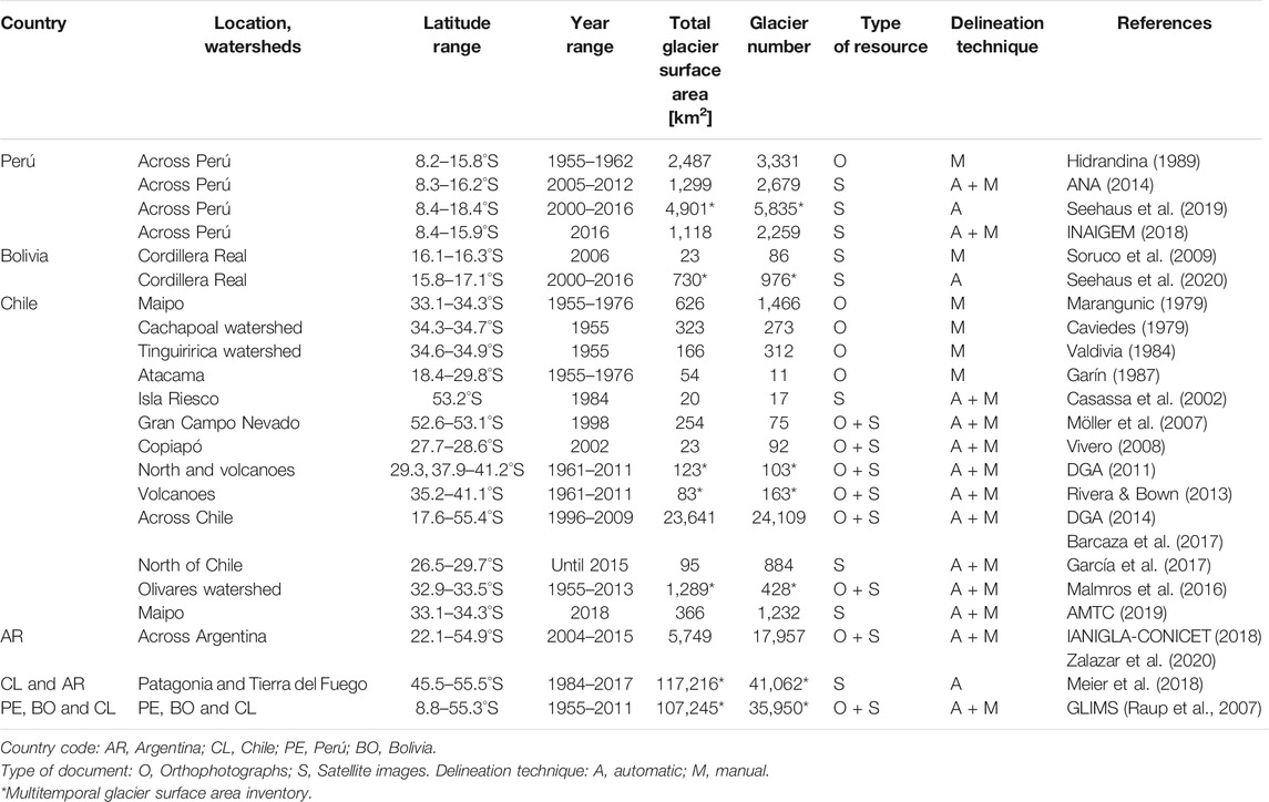
TABLE 1. List of different glacier inventories is used to generate the multi-temporal glacier surface areas dataset across the Andes between 8–55°S.

2.1.2 Glacier Inventories Merging

Based on the most recent glacier inventories made by a government initiative in Perú, Chile and Argentina (ANA, 2014; DGA, 2014; IANIGLA-CONICET, 2018), which are hereafter called the national glacier inventories (NGIs), and the Seehaus et al. (2020) glacier inventory in Bolivia. For Argentina, we do not consider some missing glaciers outlines in the inventory (without polygons), located in the Patagonian ice-field, due to this, the total glacierized area will decrease. It was possible to generate a merged product with glacier outlines from these four Andean countries, where each glacier has an identifier (ID). This ID allows to extract information from each glacier, such as: coordinates of the centroid, glacier surface areas (and corresponding dates), elevation (maximum, minimum and mean) and aspect (Degree). The slope variable (Degree) was extracted for each glacier from the Shuttle Radar Topography Mission (SRTM) v4.1 product with a pixel size of 100 m (Farr et al., 2007). Here, the surface slope of all glaciers was estimated with the DEM in order to have values quantified in the same way, since no slope data are available for some inventories.

The following procedures and limitations were applied: 1) the glacier inventories were processed in the World Geodetic System (WGS84) and the slope data was extracted using Universal Transverse Mercator (UTM) coordinate system; 2) a glacier is considered to be a polygon found entirely within a single watershed, so that the same glacier cannot be located in two or more watersheds; and 3) rock glaciers and debris-covered glaciers were not considered.

2.1.3 Glacier Area Variation Algorithm

The multi-temporal glacier surface areas dataset (Table 1) is used to apply a linear regression for each glacier (surface area = f (time)), where glacier areas per each year until 2018 were used. In order to have a homogeneous dataset across the Andes, we consider the surface area changes over the 1980–2019 period from linear regression of multi-temporal glacier surface areas (glacier outlines) identified in the national glacier inventories. For each glacier, we obtained the slope of linear regression and a coefficient of determination that are both used to evaluate the regressions. After that, we only retain the glaciers that meet the following criteria:

- Glaciers are assumed to show a reduction in the surface area since 1980 up to 2019 (Malmros et al., 2016; Meier et al., 2018; Rabatel et al., 2011; Rivera and Bown, 2013; Seehaus et al., 2019, 2020; Soruco et al., 2009). Therefore, we keep the glaciers for which the linear regression slope between the glacier surface area and date (year) is negative. A positive slope can be found due to differences in the method used to identify glacier outlines, given that all inventories did not use the same criteria to define accumulation zone limits. An example of a positive slope is observed in the Patagonian ice-fields from Meier et al. (2018) in comparison with the Chilean glacier national inventory (Barcaza et al., 2017; DGA, 2014). Another reason for the positive slope is the source date of certain inventories, since discrepancies were observed between the Chilean and Argentine national glacier inventories versus the GLIMS inventory data.

- Taking the above information into account, glaciers that show a positive linear regression slope or a negative slope with r² < 0.7 are removed.

- Subsequently, when looking at the values of the linear regression slope (GAV rates by year), we identified high GAV rates for some glaciers. For example, if a glacier with a surface area of 3 km² shrinks to 0.01 km² within a 1-year interval (i.e., a reduction of 99.7%, which is very unlikely) the slope of resulting linear regression is -2.99 km² yr⁻¹. Due to the above, such glaciers with a linear regression slope lower than -1 were considered as outliers and consequently discarded.

- Large glaciers associated with the Patagonian ice-fields that are calving were filtered out. This criterion was chosen because most of the contours of these glaciers show high differences in accumulation zones, where we cannot discriminate if glacier reduction is for differences in accumulation zones or for frontal retreat. In addition, for these glaciers, the water temperature is an important calving process (Sakakibara et al., 2013; Sakakibara and Sugiyama, 2014), that we have not considered in our study.

These filters allowed to obtain GAV data for 4,865 glaciers out of a total of 9,229 glaciers analyzed, where the average number of data used per glacier for estimate GAV was four outlines (polygons). The mean statistical significance (p-value) of GAV was < 0.001.

2.2 Glacier Mass Balance

The average annual glacier-wide mass balance for each glacier was recalculated for the 2000–2018 period from the glacier change elevation produced by Dussaillant et al. (2019) using ASTER stereo images and applying the ASTERiX methodology. In contrast with Dussaillant et al. (2019), who used the Randoph Glacier Inventory (RGI Consortium, 2017) to calculate the glacier-wide mass balance, we used glacier outlines from the national glacier inventories compiled for Perú, Bolivia, Chile and Argentina (8–55°S). The specific glacier mass balance (mb) was estimated using the glacier surface elevation change by cell (∼30 × 30 m) and a glacier ice density of 900 kg/m³ (Cuffey and Paterson, 2010). Finally, in order to obtain a comparative indicator of mass change we calculated the glacier mass balance per glacier ( $G M B_{n}$ ) as the addition of mb (Eq. 1).

G M B_{n} = \sum_{i = 1}^{n} m b_{i} (1)

In addition, we did not extrapolate the glacier change elevation for data gaps which occur in some glaciers of the Patagonian ice-fields. The mass balance uncertainty per glacier was estimated using the random error methodology that considers uncertainties on surface elevation change, glacierized area and the volume to mass conversion factor (Brun et al., 2017). In the supplementary material, the GMB derived by Dussaillant et al. (2019) and the ones from the present study are compared considering 1° latitudinal ranges.

2.3 Terra Climate Dataset

The TerraClimate dataset comprises a global dataset based on reanalysis data since 1958, with a 4 km grid size at a monthly time scale. This dataset was validated with the Global Historical Climatology Network using 3,230 stations for temperature (r = 0.95; mean absolute error 0.32°C) and 6,102 stations for precipitation (r = 0.90; mean absolute error 9.1%) (Abatzoglou et al., 2018). Here, variables such as the mean temperature, maximum temperature, minimum temperature and precipitation were processed. Based on these four variables, we calculated monthly averages for the periods 1980–2019 and 2000–2018, resulting in 36 (except mean temperature) and 48 climate variables, respectively. These variables were extracted for each grid cell where a glacier was found.

A monthly scale was necessary in order to be able to consider the seasonal differences across the Andes. Most of the glaciers are contained in a single TerraClimate cell, however, for the large glaciers of the Patagonian ice-fields, we only consider cells that encompass the centroid of those glaciers. Mean temperature was estimated from the maximum and minimum monthly temperatures. The mean temperature was not considered for the GAV analysis because the LASSO method should not have more variables than glaciers as samples in linear regression. Below, we show that smallest number of samples by watershed are 35 glaciers for the GAV analysis. For precipitation, we consider snowfall and rainfall together, i.e., we do not perform a phase discrimination using a temperature threshold.

2.4 Explanatory Variables of GAV and GMB

2.4.1 Data Pre-processing and Watershed Delineation

Morphometric and climate variables extracted from the national glacier inventories and TerraClimate dataset allowed to create two matrices for GAV (1980–2019) and GMB (2000–2018), respectively. The spatial domain at which the GAV and GMB analyses are carried out is the watershed. The watersheds were estimated using the ArcGis v10.6 software. The SRTM v4.1 product with a 100 m resolution (Farr et al., 2007) allowed estimating watershed contours by means of the flow direction and accumulation modules. For the Chilean Patagonian islands, we used the watershed classification provided by the Dirección General de Aguas of Chile (Benítez, 1978). Overall, we identified 274 watersheds with a surface area ranging from 260 to 8,095 km² (mean 2,058 ± 1,271 km²), with a glacierized surface area > 0.01% and hosting at least 10 glaciers. Each watershed has an identification (ID) associated with the glacier central coordinates (centroid).

2.4.2 Explanatory Variables Estimation Using the LASSO Method

Correlations between variables with respect to GAV and GMB for each glacier at watershed scale were estimated through LASSO (Tibshirani, 1996) on at least 35 and 50 glaciers by watersheds for GAV and GMB, respectively. This consideration is associated with the existence of glacier change data inside of each watershed, and because LASSO needs a sample minimum greater than a number of predictive variables of GAV and GMB. Recently, Bolibar et al. (2020) and Davaze et al. (2020) have shown satisfactory results using this algorithm in the Alps but at glacier scale and using temporal series. Classical linear regression methods calculate a coefficient values that maximize the r² value and minimize the error using all available explanatory variables, which results in a high variance and low bias model. The LASSO algorithm trades some of variance with bias to reduce the predictive error and to discard variables that do not explain a sufficient amount of variance in data. To reduce the prediction error, the cross-validation (CV) method is applied, which allows to select an optimal value of lambda penalty parameter. It consists of choosing a set of values for lambda where the error is calculated for each value and lambda value that gives least error is chosen. Afterward, the model is used with a chosen lambda value. We used the package “glmnet” in R to implement the LASSO algorithm (Friedman et al., 2010; Simon et al., 2011), considering 80% of data for training and remaining 20% to evaluate the error at watershed scale. Because no test method exists yet to evaluate the LASSO algorithm performance (Lockhart et al., 2015), we used the root mean square error (RMSE) derived from the LASSO algorithm to evaluate the results and we implemented the p-value test from the multiple linear regression method (MLR) to evaluate statistical significance of variables selected by the LASSO algorithm.

Additionally, to analyze the explanatory variables contribution of GAV and GMB at cluster and classic zone scales, we group the monthly climate variables selected by the LASSO algorithm to a single one, where the percentage of variance explained by each monthly variable will be combined. For example, OT3 (with data from seven watersheds for GMB) groups 25 values of morphometric and monthly climate variables, repeating some variables between watersheds, but identifying 15 unique variables for the whole cluster. In each watershed, the sum of each variable’s value contributes 100% to the explained variance (r²). Subsequently, the percentages of repeated climatic variables are added where, for example, monthly values of P_Jul present in three watersheds (three values) will be added and called P_Jul. As a result, the 25 variables’ value become 15 and when added together contribute 100% of the explained variance. In summary, precipitation variables (composed of 9 monthly values) contribute 82% to the GMB variance in OT3, followed by slope (13%), surface area (2%), and other variables (3%).

2.5 Clustering Analysis to Define New Glaciological Zones Derived From the Explanatory Variables of GAV and GMB

A clustering analysis is used to group together glacierized watersheds with similarities by taking the relevant morphometric and climate variables of the GAV and GMB analysis into account. In order to do this, we use the Partitioning Around Medoids (PAM) algorithm (Kaufman and Rousseeuw, 2008), and the Hopkins and Gap statistical methods were used to estimate clustering tendency and optimal number of clusters, respectively (Lawson and Jurs, 1990; Tibshirani et al., 2001). We used the package “cluster” in R to implement the PAM algorithm (Maechler et al., 2021), organizing variables in columns and watersheds in rows to run the PAM algorithm and all subsequent tests. The Hopkins method shows a value of 0 when a dataset is optimal for performing a clustering analysis, whereas a value of 1 shows that data is already clustered. We used this test to show the high diversity between glacierized watersheds across the Andes. In hydrology, homogeneous hydro-meteorological regions are commonly identified using a clustering analysis to transfer information toward ungauged watersheds, assuming a similarity approach. For example, the fuzzy clustering algorithm uses climate variables to determine homogeneous regions (Hall and Minns, 1999; Dikbas et al., 2012; Sahin and Kerem, 2012; Bharath and Srinivas, 2015; Matiu et al., 2020). Sometimes, geomorphological variables are also considered (e.g., Pagliero et al., 2019). Inside the fuzzy clustering algorithm, the PAM algorithm divides a dataset into groups where each one is represented by one of data points in the group. These points are called a medoids cluster, which is an object within a cluster for which average difference between it and all other clustering members is minimal (Kaufman and Rousseeuw, 2008; Lee et al., 2020). This method, using k-medoids, represents an improvement on the k-means algorithm; it is less sensitive to outliers because it does not use an average as central object (Arora et al., 2016; Lee et al., 2020). Finally, explanatory capacity of each variable in the GAV and GMB represented variances is given for each watershed and then at cluster scale.

Considering the sensitivity of the watersheds to cluster assignment by the PAM algorithm, we performed a sensitivity analysis associated with the removal of variables or group of variables and also by changing the variable values. Considering 1,000 iterations of the PAM algorithm, in each iteration, different variables were removed from the dataset. For example, monthly Tmax, then monthly Tmin and after monthly precipitation were excluded, then morphometric variables were also excluded one by one. On the other hand, in each new iteration the variable values were increased or decreased considering factors between 0.9 and 1.1. Factor values were random for each variable associated with a watershed and were updated for each new iteration. The evaluation was conducted using 274 watersheds and considering comparisons between the PAM runs (the most frequent assignment of a cluster to a watershed) using: 1) only climatic variables, 2) only morphometric variables, and 3) morphometric and climatic variables (removing one variable or a group of variables at each PAM iteration), in relation to each single PAM run removing one morphometric variable or a group of climatic variables. This means that each single PAM run removing one morphometric variable or a group of climatic variables were evaluated with regards to (i), (ii), and (iii) through the coefficient of determination.

2.6 Methodological Workflow

This section considered the next overall steps: In step 1) “Glacier area variations 1980–2019”, the glacier inventories used to identify each glacier and how its surface area has changed are used. The morphometric variables (surface area, elevation and aspect) are extracted from these inventories and from SRTM data (slope). In step 2) “Glacier mass balance 2000–2018,” the procedure used to obtain glacier mass change data based on the ASTERIX product (e.g., Dussaillant et al., 2019) is applied. In step 3) “Morphometric-climatic variables matrix”, the monthly climate values (precipitation and temperature) are extracted and implemented in a matrix with the morphometric variables. In step 4) “Explanatory variables of GAV (4a) and GMB (4b)”, the matrix of variables is used to derive relationships to explain GAV and GMB through the LASSO algorithm. In step 5) “Clusters”, a clustering analysis is carried out based on the explanatory variables of GAV and GMB.

Figure 1 illustrates the methodological workflow used in this study. It is composed of five steps that are first used to identify the explanatory variables for GAV over the 1980–2019 period and GMB over the 2000–2018 period. Then, the workflow allows to cluster watersheds based on the explanatory variables of recent glacier changes from the Outer Tropics to Tierra del Fuego (8–55°S).

FIGURE 1

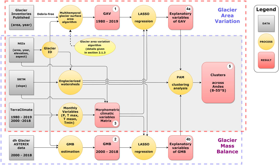
FIGURE 1. The workflow to obtain the explanatory variables of the glacier area variation (GAV) and glacier mass balance (GMB) spatial variances is presented. The final results are used to estimate clusters between 8–55°S using the explanatory variables of glacier changes. The numbers from 1 to 5 refer to the 5 steps described in the text.

3 Results

3.1 Morphometric and Climate Settings

From the national glacier inventories, we considered and identified 44,853 glaciers with a total glacierized area of 29,387 km² between 8 and 55°S. Of this glacierized surface area, 95% (33,000 glaciers, 27,793 km²) corresponds to free-of-debris glaciers, while 3% (10,881 glaciers, 1,041 km²) are rock glaciers (not considered in this study) and 2% (972 glaciers, 552 km²) are debris-covered glaciers (not considered in this study). Within the studied countries, Chile has the largest glacierized area comprising 78% of the total, followed by Argentina (16%), Peru (5%) and Bolivia (1%). Due to data lacks on glacier outlines of the Southern Patagonian Icefield (on the Argentinean side mainly), these were not considered in this analysis. Therefore, our final sample contains 85% (31,963) of glaciers covering 71% (24,888 km²) of the glacierized surface area across the Andes identified here.

Following the classic zones defined based on former studies (Troll, 1941; Lliboutry, 1998; Masiokas et al., 2009; Sagredo and Lowell, 2012; Barcaza et al., 2017; Dussaillant et al., 2019; Zalazar et al., 2020), 72% of the glacierized area are concentrated in South Patagonia and North Patagonia between 42 and 53°S, where glaciers have a mean elevation of 1,560 m a.s.l. The Tierra del Fuego zone (53–55°S) concentrates 14% of the glacierized area with a mean elevation of 830 m a.s.l. The longest latitudinal extent north of the North Patagonia include zones from the Outer Tropics to the Lakes District (8–42°S) which only contains 14% of the glacierized area. Along this extent (8–42°S), the Outer Tropics (8–17°S) and the Central Andes (30–37°S) zones contain 6% of the glacierized area each. The highest mean elevations of glaciers are found in the Desert Andes (5,575 m a.s.l.) followed by the Outer Tropics (5,177 m a.s.l.).

From a climatic point of view, the mean annual temperature over the 1980–2019 period at glacier elevation tend to decrease from the Outer Tropics (3.2°C) to the Central Andes (-2.7°C). Southward of the Lakes District, the mean annual temperature increases (5.4°C) above the values found in the north and then decreases toward Tierra del Fuego (3.8°S). With regards to precipitation, the mean annual amount decreases from the Outer Tropics (912 mm yr⁻¹) to the Dry Andes (151 mm yr⁻¹), from where it increases to Southern Patagonia (1,770 mm yr⁻¹). Southward, Tierra del Fuego shows a lower amount of precipitation, even less than the Lakes District (1,105 mm yr⁻¹). In addition to observed morphometric and climatic differences between the classic zones, it is also possible to identify major differences inside these zones at grid scale (1 × 1°) as shown in the supplementary material (Supplementary Figure S1 and Supplementary Figure S2).

3.2 Glacier Surface and Mass Loss

Across the Andes between 8 and 55°S, the mean GAV was estimated to be -31.2 ± 0.6%. This was quantified from data available on 21% (5,160 km²) of the glacierized area across the Andes (Figure 2A). The Outer Tropics showed a reduction of −41 ± 0.01% whereas a reduction of −30 ± 0.6% was found for the Southern Andes. For these two regions, these estimates are based on 50 and 19% of the glacierized area, respectively. In the Southern Andes, the Desert Andes (17–30°S) shows the largest shrinkage (−53 ± 0.002%), followed by the Central Andes (30–37°S) with a GAV of −39 ± 0.01%. In the Wet Andes (37–55°S), the Lakes District shows a GAV of −52 ± 0.1%, followed by North Patagonia (−32 ± 1.3%), South Patagonia (−28 ± 1.4%) and Tierra del Fuego (−24 ± 0.4%). For these GAV estimates, the proportion of glacierized area considered varies from one zone to another, comprising 23% of the glacierized area in the Central Andes, 20 and 13% in North and South Patagonia, respectively, and 33% in Tierra del Fuego. In smaller glacierized zones of the Andes (representing 2% of the total), GAV estimates for the Desert Andes and the Lakes District is based on 13% of the glacierized area. Regarding GAV statistical significance, the mean p-value was < 0.001. However, 11 of 48 latitudinal ranges from 8 to 55°S showed p-values > 0.05. These are located at 12–14°S, 15–16°S, 18°S, 36°S, 38°S, 40°S, and 46–47°S.

FIGURE 2

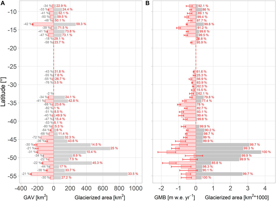
FIGURE 2. The latitudinal GAV (1980–2019) and GMB (2000–2018) across the Andes (8–55°S) are presented in this figure. (A) For each 1° latitudinal bar of GAV (red bars) the GAV error (red lines), and percentage of the mean GAV (gray texts) are presented, while the glacierized area used in GAV estimation (gray bars), as well as the percentage of this glacierized area with regards to the total estimated by the national inventories (red text) are shown. (B) The GMB (red bars), the GMB error (red lines), and the related glacierized area (gray bars) are presented, indicating the percentage of the glacierized area used in the GMB estimation with regard to the total estimated in the national inventories (gray text). The GMB estimation contains 96% (23,978 km²) of the glacierized area distributed between 26,856 glaciers considered in this study.

Additionally, the GMB is estimated to be -0.82 ± 0.12 m w.e. yr⁻¹ when considering 96% (23,978 km²) of the glacierized area of the Andes between 8 and 55°S (Figure 2B). The Outer Tropics show a lower mass loss (−0.47 ± 0.03 m w.e. yr⁻¹) compared to the southern Andes (−0.84 ± 0.13 m w.e. yr⁻¹). In the Dry Andes, the Central Andes show a greater loss (−0.43 ± 0.05 m w.e. yr⁻¹) compared to the Desert Andes (−0.22 ± 0.03 m w.e. yr⁻¹). In the Wet Andes, North Patagonia presents the greatest loss with −0.96 ± 0.18 m w.e. yr⁻¹, followed by South Patagonia (−0.9 ± 0.27 m w.e. yr⁻¹), the Lakes District (−0.72 ± 0.08 m w.e. yr⁻¹), and Tierra del Fuego (−0.56 ± 0.24 m w.e. yr⁻¹). The proportion of glacierized area considered to estimate that GMB is greater than 94% in most of the zones, except in the Central and Desert Andes where these percentages are 72 and 47%, respectively. Table 2 summarizes GAV and GMB for the classic zones, while differences observed in the GMB estimation by this work, Dussaillant et al. (2019), Braun et al. (2019) and Seehaus et al. (2019, 2020) are shown in the supplementary material (Supplementary Figure S4 and Supplementary Table S1).

TABLE 2

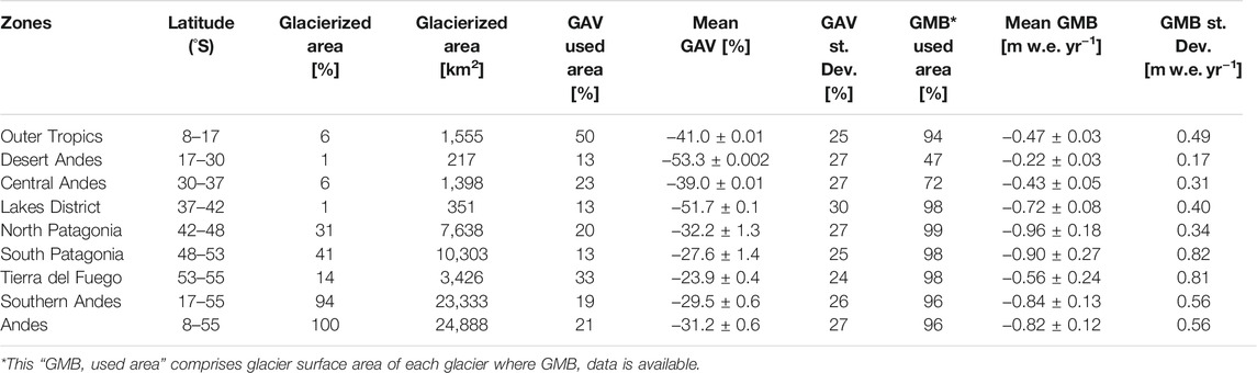
TABLE 2. GAV (1980–2019) and GMB (2000–2018) for the classic zones of the Andes.

Regarding the relationship between GAV and GMB at watershed scale (n = 107; for 3,978 glaciers with a minimum of 10 and maximum of 176 per watershed), Figure 3 shows that even if the two variables are statistically correlated for several watersheds (mostly located in the Southern Andes between 45 and 50°S), no correlation is found across the Andes. This result justifies identifying separately the morphometric and climate controls for GAV and on the other hand for GMB, considering that the GAV and GMB data include different time ranges with different response times and glacier dynamics.

FIGURE 3

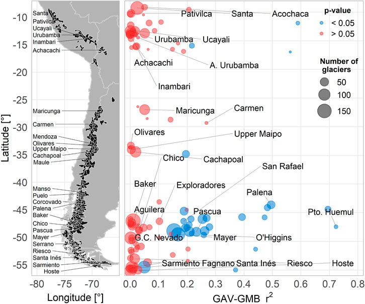
FIGURE 3. The distribution of the 274 glacierized watersheds (glacier cover > 0.01%) across the Andes (8–55°S) and the GAV (1980–2019) and GMB (2000–2018) correlation at watershed scale for 107 watersheds are presented, with its statistical significance and number of glaciers considered in each watershed.

3.3 Explanatory Variables of Glacier Changes Across the Andes

The explanatory capacity of variables on the spatial variance of GAV (1980–2019) and GMB (2000–2018) in Perú, Bolivia, Argentina, and Chile were obtained from 35 watersheds for GAV and from 110 watersheds for GMB (Figure 4A) through the LASSO method. The watersheds where the GAV variance was predicted show a mean coefficient of determination of 0.49 (RMSE = 0.85 km²; p-value from MLR < 0.05; number of glaciers = 2,484). The lower number of glaciers considered here with regard to the total GAV data (4,865 glaciers) is due to removal of watersheds that do not have a glacierized area > 0.01% of watershed area and a minimum of 35 glaciers. For the remaining 35 watersheds, the LASSO algorithm identified 39 explanatory variables for the GAV dataset. However, this number of explanatory variables differs between watersheds, with a maximum of 21 variables identified by LASSO in some watersheds. Similarly, the GMB analysis considered a minimum of 50 glaciers per watershed, resulting in a mean coefficient of determination of 0.35 for the 110 watersheds (RMSE = 0.35 m w.e. yr⁻¹; p-value from MLR < 0.05; number of glaciers = 20,740) (Figure 4B). The reduction in the number of glaciers (from 31,963 to 20,740) used in the LASSO analysis was due to the smallest number of glaciers considered by watershed. For these 110 watersheds, the LASSO algorithm identified 54 explanatory variables (43 explanatory variables in certain watersheds). These results are presented for the classic zones in the supplementary material (Supplementary Table S2), while the coefficient of determination for LASSO and MLR (p-value) results are shown in Supplementary Figure S5.

FIGURE 4

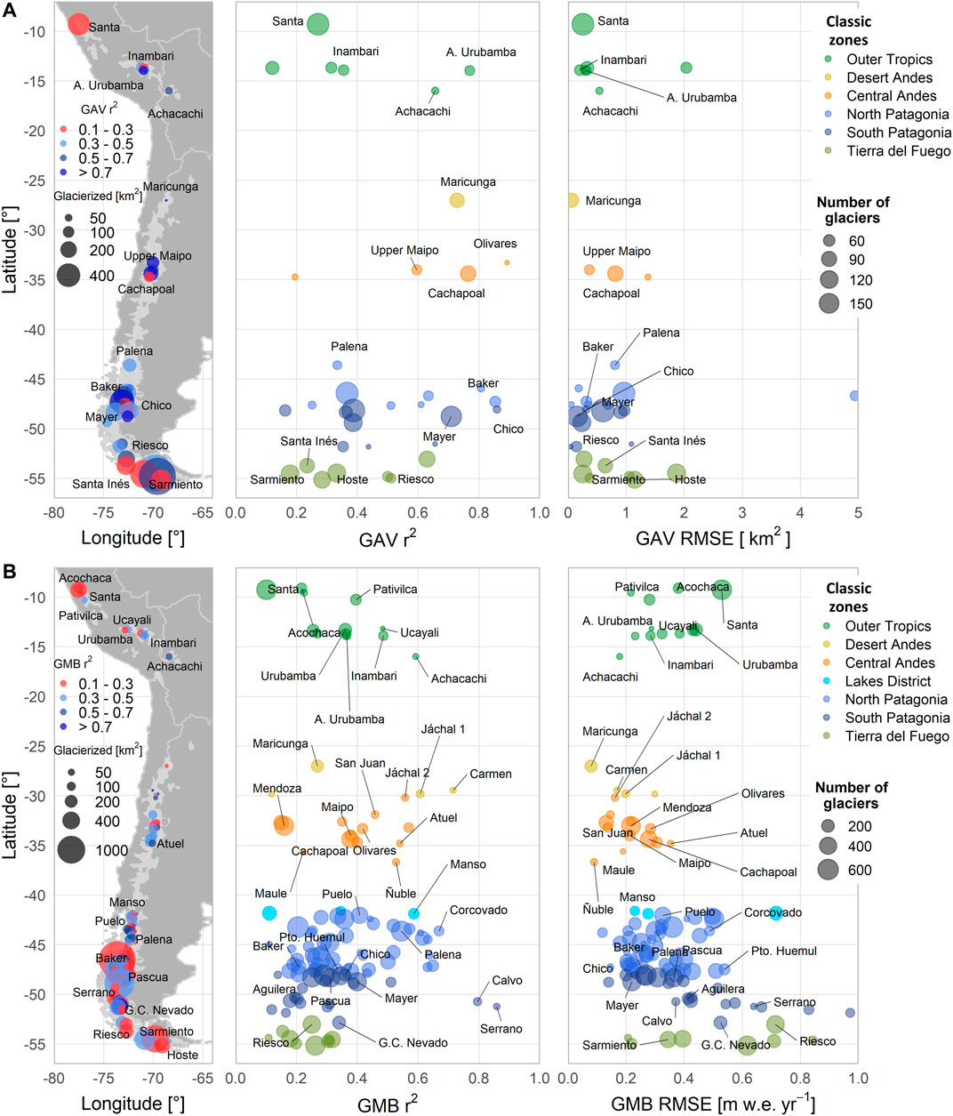
FIGURE 4. The coefficient of determination and RMSE values are presented for 35 watersheds using the GAV 1980–2019 data (A) and for 110 watersheds using the GMB 2000–2018 data (B). The values for each watershed were obtained through the LASSO algorithm, which identified the explanatory variables of the GAV and GMB spatial variances. All 274 glacierized watersheds (> 0.01%, number of glaciers >10) identified here are presented (clear gray).

Based on the 39 variables that explain the GAV variance, on average for the entire study region (8–55°S), the morphometric variables such as surface area (16%) and elevation (7%) are those that contribute most, whereas highest contribution of a climate variable is only 5% (Tmax_Jan). However, if we combine the contribution of monthly climate variables to the GAV variance, the order of explanatory variables changes (e.g., the contribution of monthly climate variables are combined in a single percentage for precipitation, Tmax and Tmin). As such, the climate variables explain 65% of the GAV variance (with temperature and precipitation contributing 35 and 30%, respectively), whereas surface area and elevation explain 16 and 15% of variance, respectively, followed by slope (4%) and aspect (1%). Looking at the GMB variance, on average across the Andes, surface area of glaciers (26%) is the variable that contributes highest percentage, followed by Tmax_Nov (5%) and slope (3.5%), with P_Apr contributing only 3.3%. As observed for GAV, when monthly explanatory variables are combined, the order of explanatory variables with regards to the GMB variance changes. Therefore, the climate variables explain most of the GMB represented variance with 66% compared to the morphometric variables, with temperature contributing 37% and precipitation contributing 29% of the represented variance. Surface area is the morphometric variable that contributes highest percentage to the GMB variance (26%), followed by elevation (4%), slope (4%) and aspect (0.2%).

3.3.1 New Classification Zones of Andean Glaciers

We performed a cluster analysis based on 274 watersheds (31,963 glaciers) using the explanatory variables selected by the LASSO algorithm. Considering the assumption that variables that explain the glacier change spatial variance in 35 watersheds for GAV and in 110 watersheds for GMB can explain glacier change in rest of Andean watersheds, we use 42 relevant variables selected by LASSO for the GAV and GMB datasets. These 42 variables are 12 monthly values for three climate variables (precipitation, Tmax and Tmin) and six values for morphometric variables (area, slope, aspect, max. elevation, min elevation and mean elevation). Tmean variable was not considered because it showed lowest explanatory capacity of the glacier changes spatial variance. According to the Hopkins method, our dataset shows a high potential to form clusters (the Hopkins test result is equal to 0.1), while the GAP statistic method allowed to quantify the cluster optimal number as 12. Concerning to the PAM algorithm sensitivity, PAM runs using climatic variables and morphometric-climatic variables showed a lower explained variance by the predictors if precipitation or Tmax variables are removed (see Supplementary Figure S6 in the supplementary material). This means that the cluster assignment of each watershed changes more if these two variables are not present in the cluster analysis. In comparison, the removal of morphometric variables and Tmin showed PAM runs with greater explained variances, meaning that the cluster assignment of each watershed is less sensitive to the removal of these variables. In contrast, PAM runs using only morphometric variables showed a lower explanatory capacity of the variance, associated with an increase of the change to the cluster assignment of each watershed. About increase and decrease of the variable values between 0 and 10%, a way to add uncertainty to variable values, it was not observed any change in the cluster assignment of each watershed.

One cluster in the Outer Tropics (OT1) does not have data of GAV and GMB in some watersheds for estimating the explanatory variables of glacier changes. However, this zone is different from the two others in the Outer Tropics (i.e., OT2 and OT3) due to lower extreme temperature and mean glacier size values, for example. These numeric results are presented in the supplementary material (Supplementary Table S3).

Figure 5A shows the map that results from the clustering. A clear latitudinal distribution can be seen between 25°S and 40°S, with some overlaps resulting from similar morphometric and climatic configurations between watersheds located on eastern and western sides of the Andes. Here, one interesting latitudinal overlap example can be observed in Dry Andes. A watershed located in DA3 (id = 25,001; p = 185 mm yr⁻¹; elevation = 6,039 m a.s.l.) close to DA1 watersheds (id = 26,426; p = 79 mm yr⁻¹; elevation = 5,753 m a.s.l.) shows higher precipitation and elevation. However, in the Outer Tropics and the Wet Andes the clusters in general are not delimited with respect to latitude. An exception is the WA2 cluster, which covers watersheds west and east of the mountain range. Watersheds that show similar morphometric and climatic configurations are clustered even if they are not contiguous to one another. An example of this can be seen from watersheds inside W5 and W6 clusters, where they present close values of aspect, slope, and elevation, even the temperature values are close, but the precipitation presents high differences within the clusters even higher than between the two clusters. In addition, Tierra del Fuego is longitudinally split into two clusters (WA4 and WA6).

FIGURE 5

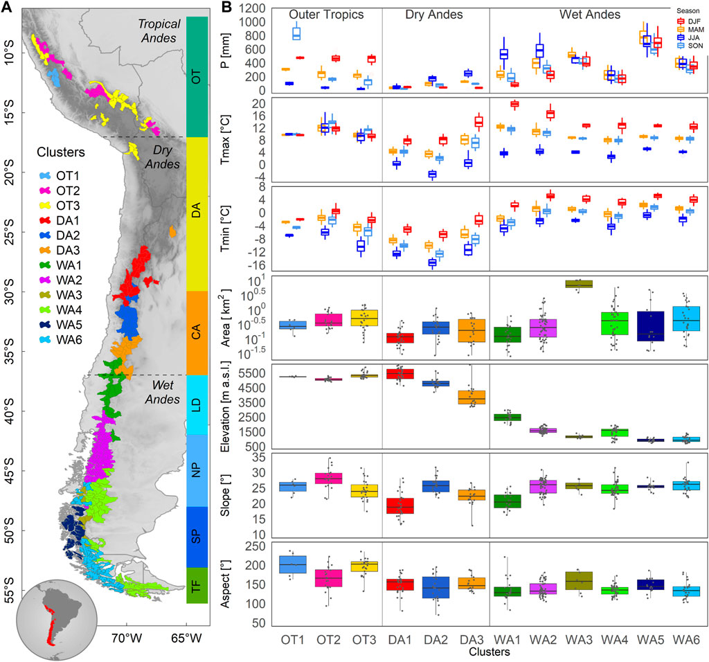
FIGURE 5. The 12 clusters of the glacierized watersheds across the Andes (8–55°S) and the behavior of climatic and morphometric variables. The average values of variables (for 274 watersheds and using 31,963 glaciers) are presented for the 12 clusters identified (PAM algorithm) using the GAV and GMB explanatory variables (LASSO algorithm). These clusters are found in three regions: Outer Tropics (OT; 8–17°S), Dry Andes (DA; 17–37°S) and Wet Andes (WA; 37–55°S). (A) shows the cluster distribution across the Andes and the classic zones, from north to south are: Outer Tropics (OT; 8–17°S), Desert Andes (DA; 17–30°S), Central Andes (CA; 30–37°S), Lakes District (LD; 37–42°S), North Patagonia (NP; 42–48°S), South Patagonia (SP; 48–53°S) and Tierra del Fuego (TF; 53–55°S). (B) presents the climatic variables (1980–2019) which are grouped into the summer (DJF), autumn (MAM), winter (JJA), and spring (SON) seasons for the Southern Hemisphere. The sum of the precipitation and the extreme temperatures averages are shown here. Additionally, morphometric variables associate with the glacierized area (i.e., surface area, elevation, slope, and aspect) are shown.

Figure 5B provide more details about the 12 clusters and their relevant morphometric and climatic characteristics. Considering the glacierized surface area in this work, which comprises 71% of the total surface area of the inventoried glaciers in the Andes, the Outer Tropics (8–17°S) comprise three clusters (OT1, OT2, OT3) concentrating 5.7% of the total glacierized area. OT3 contributes to 67% of the glacierized area in the Outer Tropics (3.8% in the Andes; 921 km²). OT3 includes glaciers in Peru, Bolivia and volcanoes in northern Chile and western Bolivia. Within the Outer Tropics, the three clusters show an annual precipitation range between 782 mm yr⁻¹ (OT3) and 1,654 mm yr⁻¹ (OT1), concentrated during the DJF season (up to 500 mm) in all of the clusters and with a marked dry season in JJA (less than 100 mm). Tmax shows similar values throughout the year for all three clusters, and is slightly higher in OT2 (13.1°C), whereas Tmin shows a seasonal variation with higher values in DJF (OT2; 0.3°C) than in JJA (OT3; -10.3°C). With regards to the morphometric variables, cluster OT3 shows the largest mean glacier surface area (0.6 km²), an average glacier elevation (5,335 m a.s.l.), and the lowest slope (24°). The Dry Andes (17–37°S) gather three clusters (DA1, DA2, DA3) which represent 6.7% of the total glacierized area. In this region, many glaciers (19–26°S) inside watersheds with a lower glacierized areas (glacierized watershed < 0.01%) were excluded. DA2 contains the most extensive glacier coverage with 52% (3.4% of the total for the Andes; 807 km²). Within these three clusters, the annual amount of precipitation increases southward, with 150 mm yr⁻¹ in DA1 and 483 m yr⁻¹ in DA3. Precipitation is mainly concentrated during JJA in DA2-DA3 and is more evenly distributed in DA1. The extreme temperatures show the highest values in the DJF season (both for Tmax which reaches a maximum of 14°C and Tmin which reaches a minimum of -2.3°C) and lowest values in JJA (Tmax < 0.5°C; Tmin < -11°C). The largest average glacier surface area is found in DA2 (0.3 km²) and the smallest is in DA1 (0.1 km²) where glaciers are also found at the highest elevation (5,389 m a.s.l.) and have the lowest slope (19°) of all the Andes.

The Wet Andes (37–55°S) comprise 87.7% of the total glacierized area of the Andes, distributed in six clusters (WA1 to WA6), where WA3 contains 34% (30.1% in the Andes; 7,205 km²) and WA4 29% (25.9% in the Andes; 6,194 km²) of the glacierized area in the Wet Andes. The annual amount of precipitation differs considerably between the clusters ranging from 2,858 mm yr⁻¹ (WA5) to 784 mm yr⁻¹ (WA4). Precipitation is concentrated in JJA in WA1 and WA2 (approximately 580 mm) and MAM-JJA in WA3 to WA6 (approximately 800 mm). Extreme temperatures in the Wet Andes present maximum values in DJF (Tmax of roughly 20°C and Tmin of roughly 5°C) and minimum values during JJA (Tmax of roughly 5°C and Tmin of roughly -0.8°C). With regards to morphometric variables, the largest mean glaciers size is found in WA3 (8 km²), and a decrease in the glacier mean elevation is observed from WA1 to WA6, with an average difference of 1,500 m. The slope is similar in all of the Wet Andes (25–26°) clusters although it is slightly lower in WA1 (21°).

3.3.2 Explanatory Variables at Cluster and Watershed Scale

The explanatory variables of the GAV and GMB represented variances at watershed scale are presented in detail for GAV (Figure 6) and GMB (Figure 7), using the 12 clusters. In the Outer Tropics, the explanatory variables of the GMB variance in cluster OT2 are precipitation (71%, P_Aug and P_Dec mainly) and temperature (19%). In cluster OT3, on average, the GAV variance is explained by precipitation (50%) and temperature (10%), with an increased explanatory power for precipitation (82%, mainly P_Sep and P_Oct) in the GMB variance. In OT3, for the Achacachi watershed (id = 16,031; GAV r² = 0.7; GMB r² = 0.6) P_Oct and P_Sep are most relevant for the GMB and GAV variances, followed by the surface area and slope.

FIGURE 6

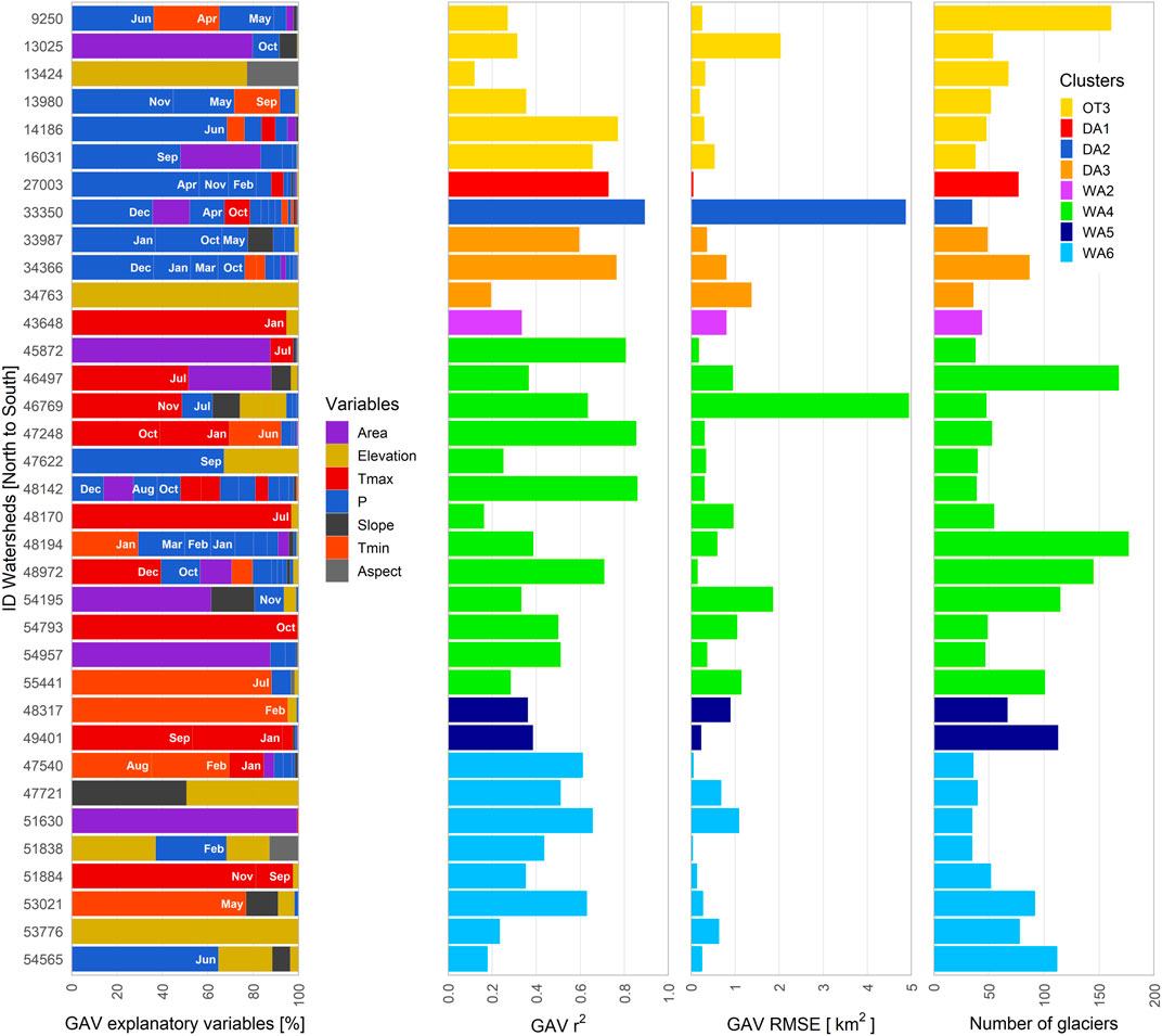
FIGURE 6. Relevance of the morphometric and climatic variables identified by LASSO algorithm to the spatial variance of GAV (1980–2019) across the Andes (8–55°S). The GAV explanatory variables, at watershed scale, is added to represent the 100% associate to each GAV r² (variance by watershed). Other relevant data as RMSE and the number of glaciers used in estimations are showed. Due to data limitation, the results are available for 8 of the 12 clusters.

FIGURE 7

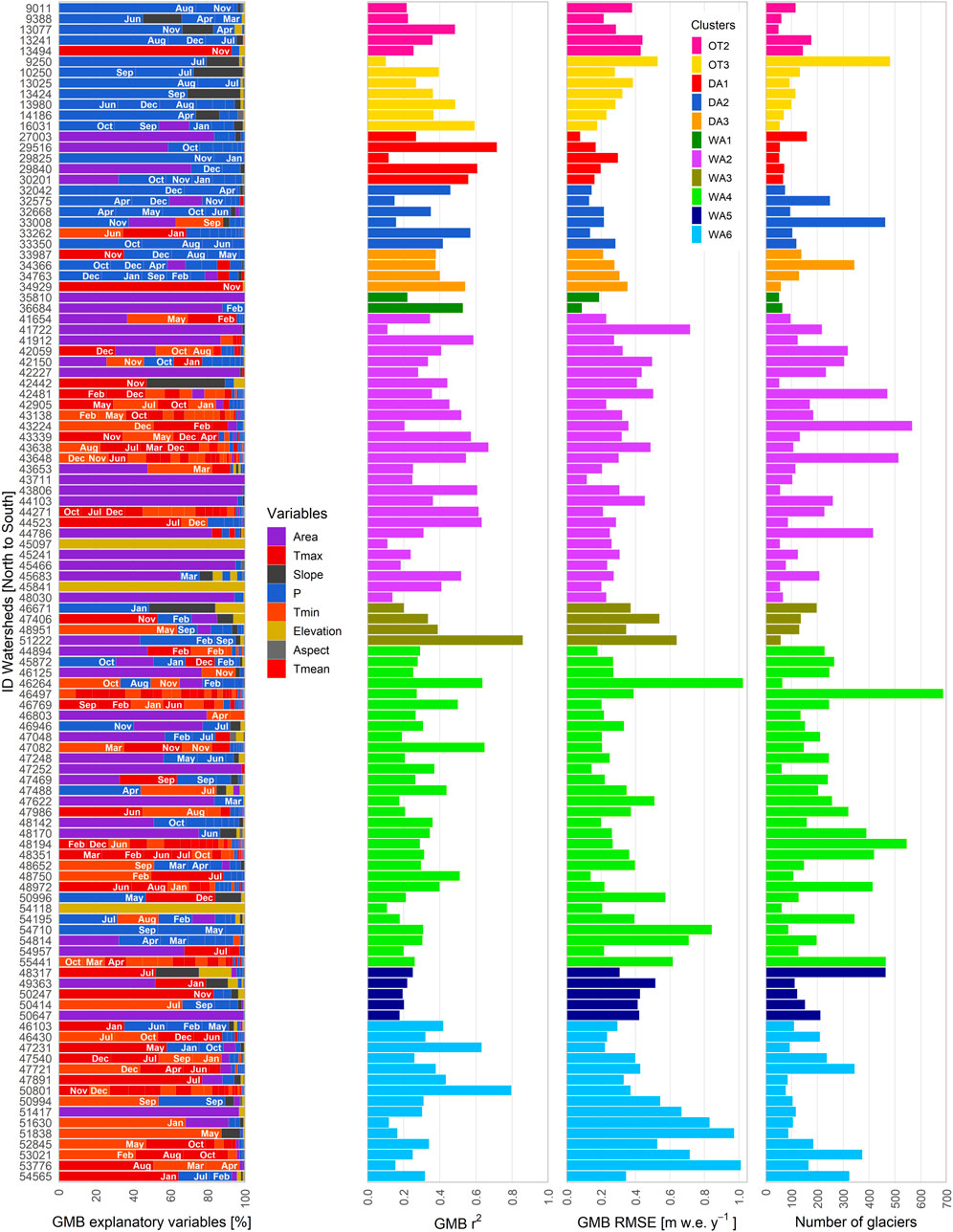
FIGURE 7. Relevance of the morphometric and climatic variables identified by LASSO algorithm to the spatial variance of GMB (2000–2018) across the Andes (8–55°S). The GMB explanatory variables, at watershed scale, is added to represent the 100% associate to each GMB r² (variance by watershed). Other relevant data as RMSE and the number of glaciers used in estimations are showed. Due to data limitation, the results at watershed scale are available for 11 of the 12 clusters.

In the Dry Andes, the explanatory variables in cluster DA1 are precipitation (93%) and temperature (5%) for GAV. The variance of GMB is mainly explained by precipitation (49%) and surface area (49%). In DA1, the Río del Carmen watershed (id = 29,516; GMB r² = 0.7) shows that precipitation and surface area have a similar contribution to the GMB variance. In cluster DA2, the explanatory variables of the GAV and GMB variances are precipitation (> 67%) followed by temperature (> 16%). One of the most glacierized watersheds of the Dry Andes is the Olivares watershed (id = 33,350; GAV r² = 0.9; GMB r² = 0.4) for which P_Dec and P_Apr and surface area explain most of the GAV variance, and P_Oct, P_Aug and P_Jun explain most of the GMB variance. In cluster DA3, the explanatory variables of the GAV and GMB variances are precipitation (> 57%), followed by elevation (34%) for GAV and temperature (37%) for GMB. In this cluster, for the Upper Maipo (id = 33,987; GAV r² = 0.6; GMB r² = 0.4) and Cachapoal (id = 34,366; GAV r² = 0.8; GMB r² = 0.4) watersheds, P_Dec (GMB) and P_Oct (GAV) are the most relevant. Whereas in the Atuel watershed (id = 34,929; GMB r² = 0.5), Tmax_Nov explains most of the GMB variance.

In the Wet Andes, the WA1 and WA2 clusters are located to the north of the Patagonian ice-fields. In WA1, the GMB variance is mainly explained by the surface area (94%) followed by precipitation (6%). Meanwhile, in WA2, the variable that mainly explains the GAV variance is temperature (95%), whereas the GMB variance is mainly explained by area (43%) and temperature (40%). The GMB variance in the Río Ñuble watershed (id = 26,684; GMB r² = 0.5), in WA1, is explained by surface area followed by P_Feb. In cluster WA2, the glacier surface area explains most of the GMB variance in the Río Manso watershed (id = 41,912; GMB r² = 0.6), and Tmax_Dec and surface area are the dominant variables in the Río Puelo watershed (id = 42,059; GMB r² = 0.4).

Clusters WA3 to WA6 are found between the Northern Patagonian ice-field and the Cordillera Darwin. Cluster WA3 comprises the largest glacierized area in the Andes (30%). Precipitation and temperature (36 and 29%) explained most of the GMB variance, followed by surface area and slope (16–13%). Close to the Southern Patagonian ice-field, in the Río Serrano watershed (id = 51,222; GMB r² = 0.9), the glacier surface area, P_Feb and P_Sep are the most statistically significant explanatory variables. In WA4, the variables that explain most of the GAV and GMB variances are temperature (40–45%), followed by surface area (24–38%) and precipitation (22–25%). This cluster contains watersheds that are primarily located to the east of the Patagonian ice-fields, and in the Cordillera Darwin to the east of Monte Sarmiento. To the east of the Southern Patagonian ice-field, the Lago O'Higgins watershed (id = 48,652; GMB r² = 0.3) shows the statistical importance of Tmin_sep and P_Mar and P_Apr. On the southern side of Cordillera Darwin (id = 54,793; GAV r² = 0.5) the main explanatory variable is Tmax_Oct, whereas on the northern side, it was found that morphometric and climatic variables had a very limited explanatory capacity (id = 54,195; GAV r² = 0.3; GMB r² = 0.2).

The WA5 and WA6 clusters are located on the western side of the Patagonian Andes. Watersheds in WA5 are mainly found to the west of the Southern Patagonian ice-field, in the coastal region where the highest amount of precipitation in the Andes was identified. For these watersheds, temperature is the most relevant variable. For example, in Río Pascua watershed (id = 48,317; GAV r² = 0.4; GMB r² = 0.3) Tmax_Jul and Tmin_Feb are important in the spatial variance of the glacier changes and in Isla Wellington (id = 50,401; GAV r² = 0.4) are Tmax_Sep and Tmax_Jan. Whereas in WA6, the explanatory variables strongly differ between GAV and GMB. The morphometric variables (30% elevation) explain 54% of the GAV variance and climate variables (73% temperature) explain 86% of the GMB variance. This cluster comprises watersheds that are primarily distributed around the Northern Patagonian ice-field and the south of the Southern Patagonian ice-field down to Monte Sarmiento, where the largest ice concentration outside the Patagonian ice-fields and Cordillera Darwin is found.

3.3.3 Explanatory Variables at the Regional Scale

Figure 8 shows the explanatory variables of GAV and GMB spatial variances at cluster scale. At first glance, it can be observed that precipitation explains the highest percentage of GAV and GMB variances for clusters located within the Outer Tropics (OT1, OT2, OT3) and the Dry Andes (D1, D2, D3), whereas temperature is most relevant variable in the Wet Andes (WA1 to WA6). Within the Outer Tropics and the Dry Andes clusters, precipitation explains between 49–93% of the GAV and GMB variances, whereas temperature only explains between 3 and 37%. In the Wet Andes, the explanatory variables of GAV and GMB variances are inverted, with temperature contributing between 29 and 73% of variation and precipitation between 1 and 36%.

FIGURE 8

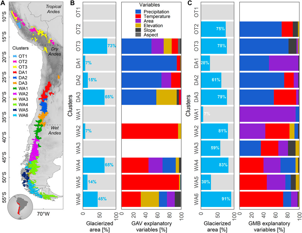
FIGURE 8. Explanatory variables of glacier changes across the Andes (8–55°S) since 1980 at watershed scale. (A) The 274 glacierized watersheds inside 12 clusters are shown on the map of South America. The glacierized area considered in estimates of the (B) GAV (1980–2019) and (C) GMB (2000–2018) explanatory variables (light blue bars) are shown with regard to the percentage of explanatory variables for the GAV and GMB spatial variances (blank spaces are due to a lack of data in that cluster).

In further detail, this explanatory power of precipitation in the Outer Tropics and the Dry Andes clusters and of temperature in the Wet Andes clusters is clear for seven clusters that concentrate 77% of the Andean glacierized area (OT2, OT3, DA2, DA3, WA9, WA10 and WA11). Other clusters show differences in the main explanatory variables for the GAV and GMB variances.

For instance, the DA1 cluster shows that climate variables (98%) predominantly explain the GAV variance, manly for precipitation (93%). On the other hand, GMB is explained in similar proportion by climate (49%) and morphometric (51%) variables, where the most important variables are precipitation and surface area with 49% each. For cluster WA1, without GAV variables identified, morphometric (94%) variables explain the GMB variance through surface area (93.9%). In WA2, temperature (95%) explain the GAV variance while the GMB variance is dominated by morphometric variables (54%) being more relevant surface area (43%) followed by temperature (40%). In WA6, 54% of the GAV variance is explained by morphometric variables (elevation alone explains 30%), and 86% of the GMB variance is explained by climate variables, where temperature explains 73%.

Finally, differences in explanatory power of morphometric and climate variables for the GAV and GMB spatial variances when considering the classic zones or the clusters can be observed in the supplementary material (Supplementary Table S4 and Supplementary Table S5).

4 Summary and Concluding Remarks

This study is the first to explore climatic and morphometric variables of the spatial variance of glacier changes through a machine learning method across the Andes (8–55°S), in terms of surface area variations since 1980 and mass balance changes since 2000. Overall, we found that the spatial variability of glacier changes is primarily controlled by spatial variability of precipitation from the Outer Tropics to the Dry Andes (8–37°S) and of temperature in the Wet Andes (40–55°S). These results, obtained at watershed scale, allowed to identify 12 new glaciological zones via a clustering analysis that depicts more details compared with the classic zones based on latitude ranges.

4.1 Overall Glacier Area and Mass Balance Variations

At the scale of the entire study region, the mean GAV and GMB were calculated at −31.2 ± 2% (1980–2019) and −0.82 ± 0.12 m w.e. yr⁻¹ (2000–2018), respectively. Our GMB estimation is close to the one obtained by Dussaillant et al. (2019) of -0.72 ± 0.22 m w.e. yr⁻¹ (2000–2018), and more negative in comparison with Braun et al. (2019) estimate (-0.61 ± 0.07 m w.e. yr⁻¹; 2000–2015), in both cases at the scale of the entire Andes. Differences between the estimates are related to the use of different glacier inventories to quantify the mass balance from glacier surface elevation differencing data and mass balance calculations. In fact, some glaciers found in the Patagonian ice-fields do not have elevation difference information in the accumulation zone, therefore our results may overestimate the negative mass balance here as we did not extrapolate the glacier change elevation data to fill the gaps, as done by Dussaillant et al. (2019). Our error estimations are lower in comparison with Dussaillant et al. (2019), possibly due to the outlines precision of glaciers identified from the national glacier inventories compared to RGI v6.0. Despite the above, and as shown in Supplementary Figure S4, considering ranges of 1° latitude between 8–55°S, we did not observe relevant differences in terms of average mass balance (< 0.3 m w.e.) in comparison with the mass balance estimated in Dussaillant et al. (2019), except between 48–49°S where we estimated a less negative mass balance.

Regarding GAV, the Desert Andes (-53 ± 0.002%) and the Lakes District (-52 ± 0.1%), which include the smallest glacierized surface areas, showed highest glacier shrinkage. The glacier shrinkage estimated here is higher than the one estimated by Rabatel et al. (2011) at -29% over the 1955–2007 period in the Desert Andes and that the one reported by Paul and Mölg (2014) at -25% over the 1985–2011 period in the Lake District, but it is worth noting that the study period are different and that we consider in the overall study period used here the decade 2010–2020 during which glacier loss in these regions has strongly increased (Dussaillant et al., 2019). Southward of 42°S, the mean GAV estimated here (-24 ± 0.4% to -32 ± 1.3%) was higher than that observed by Meier et al. (2018) (-9 ± 5%, 1986–2016): this is likely related to differences in the study periods and also because we did not consider the large calving glaciers of the Patagonian ice-fields, where we found glacier outlines inconsistences, particularly in accumulation zones; these glaciers covering an area up to 13% of the total in South Patagonia and 20% in North Patagonia. Overall, we discarded the glacier growth due to methodological limitations, but this should have a limited impact because many studies have described a general glacier shrinking across the Andes (e.g., Malmros et al., 2016; Meier et al., 2018; Paul and Mölg, 2014; Rabatel et al., 2011; Rivera and Bown, 2013; Seehaus et al., 2019, 2020), with few exceptions that have been reported (Rivera and Casassa, 1999; Wilson et al., 2016; Hata and Sugiyama, 2021).

Although our GAV estimates show r² > 0.7, we identified 11 latitudinal ranges in which there are low statistical significance in the relationship between GAV and morphometric or climatic variables (p-value > 0.05), concentrated mainly in the Lakes District (between 38 to 39°S and 40 to 41°S) and North Patagonia (between 42 to 43°S and 46 to 48°S).

We found that the statistical relationship between GAV and GMB is mostly non-significant across the Andes. This is not really surprising as the considered time scales for GAV and GMB are not the same and they are of different length. In addition, GAV is related to glacier response times which depends on glacier dynamics, and is therefore related to its morphometric characteristic and thus specific to each glacier. This response time may largely exceed the study period length, particularly for outlet glaciers of the Patagonian ice-fields where it can be on a secular time scale. One consequence of this absence of a relationship between GAV and GMB is that their explanatory variables were identified separately.

4.2 Main Controls of Glacier Changes

In relation to the relevant variables at watershed scale for GAV (r² = 0.5, n = 35) and GMB (r² = 0.4, n = 110), we found that, on average for the entire study region (8–55°S), climate variables explain an highest percentage of the GAV and GMB spatial variances with more than 65% (> 35% for temperature), whereas the surface area is the most relevant (> 16%) for morphometric variables. We observe a latitudinal limit from 37.5°S (DA3 in Argentina) to 39.9°S (WA2 in Chile) between the explanatory capacity of precipitation and temperature in GAV and GMB spatial variances across the Andes. Precipitation explains highest percentage of GAV and GMB spatial variances (ranging from 49 to 93% depending on the clusters) for the Outer Tropics and the Dry Andes (8–37°S), whereas temperature is the most relevant climate variable (between 29 and 73% of explained spatial variance depending on the cluster) for the Wet Andes (40–55°S). The importance of precipitation in the GMB variability had already been observed in several studies based on in situ glacier monitoring by Favier et al. (2004) and Wagnon et al. (2001) in the Outer Tropics. More specifically, Sicart et al. (2003, 2011) showed that during the transition season (Sep-Dec) when ice melt increases, precipitation frequency and intensity are key to modulating ablation because of the impact on glacier surface albedo. In the Dry Andes, no link was found between GAV or GMB which is in agreement with Rabatel et al. (2011). In addition, Rabatel et al. (2011), Masiokas et al. (2016) and Kinnard et al. (2020) pointed out the sensitivity of GMB to precipitation. For this region, we also found that glacier surface area has significant explanatory power for the GMB variance (49% in DA1), which is in agreement with Rabatel et al. (2011) who showed that small glaciers in the Desert Andes have a very negative GMB in comparison with a moderate mass loss for larger glaciers. With regards to the Wet Andes, in the Patagonian ice-fields, spatial variances of glacier changes are mainly controlled by the temperature (WA3 to WA6). This is in agreement with Abdel Jaber et al. (2019) who found that the mass loss in the Northern Patagonia ice-field is likely due to higher temperatures. Outside the Patagonian ice-fields in east (WA4), the glacier shrinkage could be explained by a temperature increase as no change in precipitation was observed (1979–2002) (Masiokas et al., 2015). In addition, Falaschi et al. (2019) found a high correlation between GMB and temperature in Monte San Lorenzo since 1958 to 2018 (temperature Oct to Mar, r = -0.86, p-value = 0.1).

4.3 Clusters Without a Latitudinal Distribution Across the Andes

In the present work, we used morphometric and climatic variables associated with GMB data for 20,740 glaciers and GAV data for 2,484 glaciers to propose a new classification that comprises 12 clusters encompassing a total of 274 watersheds and 31,963 glaciers between 8 and 55°S. This regional identification was based on the main explanatory variables of glacier changes (GAV and GMB). Up to now, only one type of classification of the glacier environments based on latitudinal ranges has been used, first by Troll (1941) and Lliboutry (1998), followed by recent studies (e.g., Barcaza et al., 2017; Dussaillant et al., 2019; Masiokas et al., 2009, 2020; Zalazar et al., 2020). Sagredo and Lowell (2012) proposed another glaciological classification with nine zones between 8–55°S; this was based on climate variables only, and with a small number of glaciers (n < 234). Here, the clusters provide a classification with greater detail allowing to better take the regional-scale diversity in the glacier characteristics and evolution into account. For instance, glaciers on volcanoes in northern Chile and western Bolivia are no longer linked to the Dry Andes but clustered with those of the Outer Tropics (OT3). In addition, watersheds located at the same latitude sometimes belong to different clusters. These results are in line with Ayala et al. (2020) who identified significant differences (GMB, runoff contribution and glacier elevation) between the southern (DA2) and northern (DA3) watersheds inside the Río Maipo watershed. With regards to the Outer Tropics and the Wet Andes, our results show that a latitudinal classification is not possible, which is in agreement with previous studies (e.g., Caro et al., 2020; Sagredo & Lowell, 2012). Southward of 46°S, we found different clusters, from west to east, related to the high contrast in precipitation and temperature amounts (WA3 to WA6) related to the wet western air masses originating from the Pacific Ocean (Langhamer et al., 2018). Studies on the Patagonian ice-fields have demonstrated this large difference in precipitation between the western and eastern sides of the cordillera (Warren, 1993; Barcaza et al., 2017; Bravo et al., 2019).

Despite these results, the sensitivity analysis showed that the absence of the variables Tmax and precipitation causes a rearrangement of the cluster assignment to each watershed, while the absence of the morphometric variables and Tmin does not show a major change in this assignment.

4.4 Implications in the Glacier Changes Simulations at the Andes Scale

Results obtained through linear machine learning method provide a new framework for glacier changes simulations across the Andes. The increase in temperature-driven and decrease in precipitation-driven glacier changes from the Outer Tropics to the Wet Andes highlights that:

a) A reduction in annual precipitation and changes in their monthly distribution will have a greater impact on glacier mass loss in the Outer Tropics and the Dry Andes in comparison with the Wet Andes. Conversely, changes in monthly temperature will be more relevant to simulate glacier mass loss in the Wet Andes.

b) The newly defined clusters will allow to orient the glacier change simulations, based on the main variables that control GAV and GMB across the Andes. For example, for regional studies across the Dry Andes to the Wet Andes, precipitation and temperature relevancies presented here can be efficiently used to estimate the mass balance, through the precipitation and ice melt factors that can be derived from numerous studies (e.g., Ayala et al., 2020; Bravo et al., 2017; Caro, 2014; Farías-Barahona et al., 2020; Huss and Hock, 2018; Masiokas et al., 2016). In this context, our results will be able to guide future regional hydro-glaciological simulations at watershed and cluster scales across the Andes.

Data Availability Statement

The original contributions presented in the study are included in the article/Supplementary Material, further inquiries can be directed to the corresponding author.

Author Contributions

AC: data processing, analysis, interpretation, and writing. TC and AR: supervision, interpretation and writing.

Funding

This study was conducted as part of the International Joint Laboratory GREAT-ICE, a joint initiative of the IRD and universities and institutions in Bolivia, Peru, Ecuador and Colombia. This research was funded by the National Agency for Research and Development (ANID)/Scholarship Program/DOCTORADO BECAS CHILE/2019—72200174.

Conflict of Interest

The authors declare that the research was conducted in the absence of any commercial or financial relationships that could be construed as a potential conflict of interest.

Publisher’s Note

All claims expressed in this article are solely those of the authors and do not necessarily represent those of their affiliated organizations, or those of the publisher, the editors and the reviewers. Any product that may be evaluated in this article, or claim that may be made by its manufacturer, is not guaranteed or endorsed by the publisher.

Acknowledgments

We acknowledge the LabEx OSUG@2020 (Investissement d’Avenir,—ANR10 LABX56). The first author would like to thank Francisca Bown (Tambo Austral), Edwin Loarte Cadenas (INAIGEM), Katy Medina Marcos (INAIGEM), Justiniano Alejo Cochacin Rapre (ANA), James McPhee (U. of Chile), Diego Cusicanqui, Jeppe Malmros, David Farías-Barahona and Thorsten Seehaus for providing the glacier inventories between the Outer Tropics and Tierra del Fuego (8–55°S), and Fernando Gimeno, Jean Carlos Ruiz Hernández, Inés Dussaillant and Vanesa Carreño for fruitful discussions on this article. Finally, we acknowledge the numerous and constructive comments and suggestions provided by the two reviewers and the Editor.

Supplementary Material

The Supplementary Material for this article can be found online at: https://www.frontiersin.org/articles/10.3389/feart.2021.713011/full#supplementary-material

References

Abatzoglou, J. T., Dobrowski, S. Z., Parks, S. A., and Hegewisch, K. C. (2018). TerraClimate, a High-Resolution Global Dataset of Monthly Climate and Climatic Water Balance from 1958-2015. Sci. Data 5, 1–12. doi:10.1038/sdata.2017.191

PubMed Abstract | CrossRef Full Text | Google Scholar

Abdel Jaber, W., Rott, H., Floricioiu, D., Wuite, J., and Miranda, N. (2019). Heterogeneous Spatial and Temporal Pattern of Surface Elevation Change and Mass Balance of the Patagonian Ice fields between 2000 and 2016. The Cryosphere 13 (9), 2511–2535. doi:10.5194/tc-13-2511-2019