Calculation of Average Reservoir Pore Pressure Based on Surface Displacement Using Image-To-Image Convolutional Neural Network Model

The average pore pressure during oil formation is an important parameter for measuring the energy required for the oil formation and the capacity of injection–production wells. In past studies, the average pore pressure has been derived mainly from pressure build-up test results. However, such tests are expensive and time-consuming. The surface displacement of an oilfield is the result of change in the formation pore pressure, but no method is available for calculating the formation pore pressure based on the surface displacement. Therefore, in this study, the vertical displacement of the Earth’s surface was used to calculate changes in reservoir pore pressure. We employed marker-stakes to measure ground displacement. We used an improved image-to-image convolutional neural network (CNN) that does not include pooling layers or full-connection layers and uses a new loss function. We used the forward evolution method to produce training samples with labels. The CNN completed self-training using these samples. Then, machine learning was used to invert the surface vertical displacement to change the pore pressure in the oil reservoir. The method was tested in a block of the Sazhong X development zone in the Daqing Oilfield in China. The results showed that the variation in the formation pore pressure was 83.12%, in accordance with the results of 20 groups of pressure build-up tests within the range of the marker-stake measurements. Thus, the proposed method is less expensive, and faster than existing methods.

Introduction

Oil reservoirs consist of porous media, and the formation pore pressure refers to the fluid pressure in the pores of a reservoir. The formation energy, development potential, rock type, and geological structure are reflected in the formation pore pressure and its variation law. Continental sandstone oilfield has entered the stage of ultra-high water cut development. With the long-term injection of foreign fluid and the continuous exploitation of oil and gas, the formation pressure is continuously supplemented and released, and the seepage law of formation fluid changes all the time. Formation pore pressure is the representation of reservoir energy and the direct embodiment of reservoir fluid seepage capacity. It also plays an important role in the adjustment of large-scale well pattern in the middle and late stage of oilfield development. The average formation pore pressure in a development block is an important parameter for adjusting the injection–production intensity and measuring the injection–production capacity (Gao et al., 2018). Accurate prediction of the formation pressure is an important prerequisite for stable and seamless oil field development (Xu W. et al., 2019; Sheng et al., 2020). During the development of an oil field, continuous casing damage occurs frequently at the weakest horizontal structural surface of the reservoir. The main reason for this phenomenon has been proven to be the slip of the weak horizontal structural surface caused by the inter-regional pore pressure. Casing damage severely affects oil field development, forcing many injection–production wells to shut in. For instance, at the Daqing Oilfield in China, an area where casing damage is prevalent, the damage rates are as high as 50–80% (Cui 2015).

The section slip of a standard horizontal fossil layer is caused by uneven deformation induced by the inter-regional pore pressure (Hu et al., 2018; Xie et al., 2020; Zhao et al., 2020). It is necessary to control the difference in average inter-regional formation pressure to prevent expansion of the casing damage area in the Daqing Oilfield (Ai et al., 2015). The original cause of the casing damage was the pressure change of the formation. Pressure changes can induce stress changes of rock underground (Guo et al., 2019a). Therefore, monitoring and prediction of the formation pore pressure are important to ensure daily oilfield production (Tang et al., 2018; Xu X. Q. et al., 2019; Tang et al., 2021). However, the average pore pressure during formation cannot be directly obtained (Shen et al., 2014; Li et al., 2017; Ameh 2019). Additionally, the formation-pressure gradient near water injection and oil production wells is excessively large to be used as the basic parameter for calculating the average formation pressure (Wang and Sheng, 2018; Zhang et al., 2020). The technology for predicting formation pore pressure has been successfully employed in seismic data prediction research since the 1970s (Tipper 1976). The main forecasting methods include the equivalent depth formula (Yun 1996), Eaton method (Eaton 1972), ratio method, empirical formula, Fillippone method (Fillippone 1982), and some other methods (Sun and Sun, 2007; Wei et al., 2007; Yu et al., 2014; Xiong et al., 2019; Zhang et al., 2021). However, these methods are limited in terms of their accuracy in calculating the seismic layer velocity. Therefore, some scholars have proposed a prediction method for abnormal formation pressure based on acoustic impedance inversion and multi-seismic attribute joint inversion (Banik et al., 2013), and based on pre-stack velocity inversion (Dutta 2002; Dutta and Khazanehdari, 2006). Moreover, the seismic multi-elastic parameter pore fluid pressure prediction method has been developed for low permeability reservoirs, and satisfactory results have been obtained in practical applications of this method (Hou et al., 2019). In general, the average pore pressure has been observed to depend on the results of pressure build-up tests, which are both cost- and time-intensive. Moreover, the pressure build-up test data of a single well can reflect the average pore pressure of only formations near the test well. Consequently, it is difficult to evaluate the average formation pressure in several oilfields.

Several studies have confirmed that a correlation exists between surface displacement and formation pore pressure, which is not a simple linear one-to-one correspondence. In 2009, Rutqvist et al. (2010) conducted a series of rock mechanics simulation analyses of a reservoir–geomechanical coupling reservoir and the interaction between pore pressure and geological stress is considered. They reported that the surface displacement was consistent with the expansion in the volume of the injection area and adjacent strata caused by the pressure change, which was as a result of the change in the reservoir pore pressure. The surface displacement depended on the change in the reservoir pressure, volume of the injected fluid, and elastic properties of the reservoir cap. Xue et al. (2018) studied the abrupt transition of the coupled gas-stress behavior at the dilatancy boundary using a strain-based percolation model. Based on orthogonal triaxial stress experiments with CH₄ seepage, the complete stress–strain relationship and the corresponding evolution of the volumetric strain and permeability were obtained. Zhang et al. (2018) investigated the effect of pore-fluid pressure on normal deformation through laboratory experiments. The results indicated that the pore-fluid pressure significantly affects the normal deformation of a jointed sample. Moreover, the relative normal deformation of the host rock during fluid injection has a linear relationship with the pore-fluid pressure. Guo et al. (2019b) considered the mechanisms of the mixed responses of unconventional reservoir under inter well interference, used the finite element method to describe the poroelastic behaviors of multiphase-fluid diffusivity and rock deformation, and used the displacement discontinuity method to describe the numerical simulation work flow of multi-fracture propagation.

Evidently, past research has focused primarily on changes in the formation pore pressure to calculate the surface displacement. Recently, surface displacement has been predicted based on underground parameters (Qi et al., 2017). However, the present study represents the first attempt at calculating the pore pressure of underground oil reservoirs based on the surface displacement. Although positive evolution is possible, reverse evolution is challenging. According to the relationship between the formation pore pressure and surface displacement, forward calculation involves an explicit equation, whereas backward calculation involves a set of equations that cannot be calculated directly. When the number of grids is large, a large number of equations will be formed. When the number of equations is large, the accuracy of the constant term of the coefficient matrix, or the input of the model, will be improved.

In this study, the convolution method was simplified to a convolution algorithm based on the convolution characteristics of the linear-deformation stage. Artificial intelligence can assist in determining the relationship between two parameters. Machine learning can play a good role in images, or two-dimensional matrix; in this regard, convolutional neural networks (CNNs) are the most effective tool. An improved CNN was established in this study to determine pore pressure variation from surface displacement. The accuracy of the model was verified using marker-stake monitoring data and the average formation-pressure data obtained from pressure build-up tests conducted in the Sazhong Development Zone, Daqing Oilfield, China.

Inversion of Changes in Average Pore Pressure

The relationship between the average pore pressure and surface displacement is critical for the inversion of the reservoir pore pressure. The surface deformation occurs only after the formation pore pressure changes. The calculation of formation pore pressure by surface deformation is an inverse calculation. The geological factors of oil layer are complex, and the formation pressure is influenced by many factors (Cipolla et al., 2018). If the value of a discrete cell in the forward calculation is the superposition of multiple equations, the inverse calculation is to solve these equations, but if the forward calculation is an iterative calculation, the reverse calculation needs multivariable iterative solution. Only forward calculation is simple enough, and inversion calculation can be carried out. The extent of the change in the reservoir volume caused by the change in reservoir pore pressure is within the range of linear elastic deformation of reservoirs. The deformation of the reservoir due to changes in pore pressure simultaneously causes deformation of the surrounding strata, and the resulting displacement is transferred to the surface. In this process, the deformation of the formation rock is still in the stage of linear elasticity. According to the superposition principle of stress and strain in the linear elastic stage, the final surface displacement is the linear superposition of the change in the pore pressure of each underground storage grid on the surface displacement generated by each grid. We assumed that there was no gradient in the plane and that the mechanical and seepage parameters were equal in the plane. Thus, if a single grid changes the surface deformation distribution due to a unit pressure, the surface displacement caused by any formation pressure can be linearly superposed based on the formation deformation generated by the unit pressure of a single grid. This method can be expressed by the convolution equation:

$\mathit{u}\left(\mathit{x}\text{, }\mathit{y}\right)=\mathit{k}\left(\mathit{x}\text{, }\mathit{y}\right)\text{* }\mathit{p}\left(\mathit{x}\text{, }\mathit{y}\right)\text{,}(1)$

where u (x, y) is the vertical displacement of the surface at point (x, y) (m); k (x, y) is the convolution kernel (m), i.e., a storage grid changes the distribution of the surface displacement caused by a unit pressure (m/MPa); and p (x, y) is the formation-pore-pressure distribution (MPa).

The actual measured or calculated formation pore pressure and surface deformation parameters constituted a plane composed of limited data point planes. It is necessary to perform plane discretization in advance and discretize the stratum plane into a finite mesh with a length of M and a width of N. The two-dimensional discrete convolution equation is

$u\left(x,y\right)=k\left(x,y\right)\ast p\left(x,y\right)={\displaystyle \sum _{i=0}^M{\displaystyle \sum _{j=0}^{N}k\left(i,j\right)p\left(x+i,y+j\right)}}(2)$

The convolution kernel k (x, y) represents the vertical displacement of a formation with changes in the unit pressure of a single grid, which can be obtained through numerical simulation. Correspondingly, p (x, y) is the formation pore-pressure distribution. Therefore, the determination of surface displacement based on formation pore pressure involves forward modeling and explicit calculation, that is, for a vertical displacement u (x, y) at any surface location, there is no unknown number in the solution process.

To obtain the pore pressure distribution of the p (x, y) formation based on the vertical displacement u (x, y) of the surface, it is necessary to solve a large set of equations in which the number of unknowns is equal to the square of the convolution kernel. However, the position of the convolution core far away from the center was almost zero (the value of the far end of the convolution core caused by the change of unit displacement and unit pressure is almost zero). Thus, inversion of the equations is impossible because some unknown coefficients in some of the equations are close to 0, which significantly affects the solution accuracy (Hwang et al., 2019; Mohammady et al., 2020).

In the calculation for deconvolution, machine learning can be used to address the problem of convolution. Because the surface displacement field is a group of plane data, it is similar to a blurred image. CNN is the most effective type of machine learning algorithm, and it uses images as the input layer. However, the calculation of changes in formation pressure based on surface displacement inversion is deduced from one field to another, which requires some changes to the existing CNN structure. A traditional CNN model is shown in Figure 1.

FIGURE 1

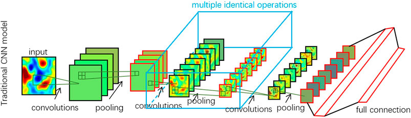
FIGURE 1. Traditional CNN model.

FIGURE 2

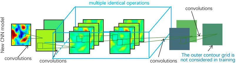
FIGURE 2. Proposed image-to-image model.

The model can be explained as equations as:

$\begin{array}{l}\text{Convolution}:h^{\left(1\right)}=I\ast k^{\left(1\right)}+b^{\left(1\right)}\\ \text{Pooling}:p^{\left(1\right)}=\text{AF}\left\{\text{POOLING}\left[h^{\left(1\right)}\right]\right\}\\ \text{Convolution}:h^{\left(2\right)}=h^{\left(1\right)}\ast k^{\left(2\right)}+b^{\left(2\right)}\\ \text{Pooling}:p^{\left(2\right)}=\text{AF}\left\{\text{POOLING}\left[h^{\left(2\right)}\right]\right\}\end{array}(3)$

where h⁽ⁱ⁾ is the i-th hidden image layer; k⁽ⁱ⁾ is the convolution kernels of i-th layer; b⁽ⁱ⁾ is the biases of i-th layer; I is the model inputs. AF is the activate function, POOLING is pooling calculation.

Pooling calculation is a computing method that divides a two-dimensional data into several regions, calculates a value from all grids in each region, and then recombines it into new two-dimensional data.

The same calculation method is used until the last convolution and pooling operation. Then each pixel of the last group of two-dimensional images is arranged into a variable h_F⁽¹⁾ in one dimension as

$\begin{array}{l}\text{Convert into one}-\text{dimensional: }{h}_{\text{F}}^{\left(1\right)}\left(m\right)=p^{\left(L\right)}\left(x,y\right)\\ \text{Full connection: }{h}_{\text{F}}^{\left(2\right)}=\text{AF}\left\{W^{\left(1\right)}{h}_{\text{F}}^{\left(1\right)}\left(m\right)+b_{\text{F}}^{\left(1\right)}\right\}\\ \text{Output: }Y\text{'}=\text{AF}\left\{W^{\left(2\right)}{h}_{\text{F}}^{\left(2\right)}\left(m\right)+b_{\text{F}}^{\left(2\right)}\right\}\end{array}(4)$

where L is the number of hidden layers; h_F⁽ⁱ⁾ is the i-th hidden layer in full connection; b_F⁽ⁱ⁾ is the biases of i-th layer in full connection; W⁽ⁱ⁾ is the weights of i-th layer; Y′ is the predicted values.

Traditional CNNs include an input layer, convolution layer, pooling layer, full-connection layer, and output layer. Through continuous convolution and pooling, the input image is abstracted into a number of low-pixel two-dimensional parameters, and the results are output through several fully connected neural networks. The output results are used for image recognition and other applications. The convolution layer is used to increase the thickness (number of images), the pooling layer is used to highlight features and reduce the number of intermediate parameters, and the full-connection layer is used to convert two-dimensional data to one-dimensional data.

For our application, the aforementioned structure must be modified. As the relationship between the fields of surface vertical displacement and formation pressure change depends on the displacement of the formation, the process is smooth and continuous. The relationship between the fields of surface vertical displacement and formation pressure change is the coupling relationship between fluid pressure and rock matrix stress in porous media. The change of rock matrix stress will cause the strain of rock, which shows macroscopic deformation and displacement on the surface. In the Seepage-solid coupling model of porous media, it can be seen from the compatibility equation derived from the geometric equation that the deformation and displacement of each point are continuous in the process of rock elastic deformation. Hence, no pooling layers are needed for image collection, and the layer thickness need not be large either. Since the output layer comprises two-dimensional data, it is an image-to-image issue, and no full-connection layer is needed to transform the dimensions of the data. Therefore, the proposed CNN does not include a pooling layer and or a full-connection layer. Pooling layer can effectively abstract and prevent overfitting in machine vision models. However, in this issue, the two functions of pooling layer are not effective. For practical physical problems, there are few features that can be abstracted as the surface deformation field does not have some contours like the image; The training data of this model comes from forward calculation, there are unlimited training samples, the training process will not encounter the same samples, so it will not overfit. At the same time, pooling computing can reduce the dimension of intermediate computing process and reduce the number of variables. However, for this problem, the number of grids becomes less after pooling, which is equivalent to a sudden doubling of the grid size, changing the corresponding relationship between the input and output layers at the same position. The proposed image-to-image model are shown in Figure 1.

The new model can be explained as:

$\begin{array}{l}{h}^{\left(1\right)}=u\ast k^{\left(1\right)}+b^{\left(1\right)}\\ h^{\left(2\right)}=h^{\left(1\right)}\ast k^{\left(2\right)}+b^{\left(2\right)}\end{array}(5)$

where u is the deformation on the ground surface, mm.

The same calculation method is used until the last convolution. The final predicted pressure change field is the final output image.

$p\text{'}(x,y)=h^{(L-1)}\ast k^{\left(L\right)}+b^{\left(L\right)}(6)$

where p' is the predicted pressure change field in reservoir, MPa.

In addition to the aforementioned modifications, the loss function of the model was adjusted. The surface vertical displacement due to changes in pore pressure at a certain underground point includes not only the point with the same plane coordinate but also the area around this point. In contrast, the vertical displacement of a certain point on the surface is the result of the joint action of pore pressure changes in a certain range of underground. The influence range of the boundary area of the underground pore pressure is larger than that of the surface vertical displacement observation area. Thus, the influence of the boundary pore pressure in the training sample cannot be fully reflected in the surface vertical displacement. In the loss function, the boundary pore pressure grid should be ignored to focus the CNN training on the relevant grid.

The CNN model requires millions of samples for training. As the surface vertical displacement can be calculated using the average formation pressure according to Eq. 2, machine learning samples can be easily obtained. The convolution kernel k (x, y) can be obtained using the finite-element method. Hence, when a certain formation pressure value is assumed, the surface vertical displacement is obtained using Eq. 2, and the corresponding average formation pore pressure and surface vertical displacement constitute a training sample. Thus, infinite training samples can be obtained by assuming different values of formation pressure and calculating the corresponding surface vertical displacements. The proposed CNN can be trained to handle practical problems using the samples thus obtained.

Oilfield Test

Forward Evolutionary Computation

In the Sazhong Development Zone of the Daqing Oilfield, the vertical displacement of the formation was measured using marker-stakes arranged on the ground and then by measuring the changes in the formation pore pressure. The marker-stakes protruded 1.5 m above the ground and extended 4.0 m into the stratum. The center of the marker-stakes was made of steel to prevent the displacement of the shallow soil. The height difference between two adjacent marker-stakes was measured using a precision level, and the vertical displacement of the stratum at each marker-stake position in the plane was calculated using four benchmark stakes in the nondevelopment area. One of the marker-stakes is shown in Figure 3.

FIGURE 3

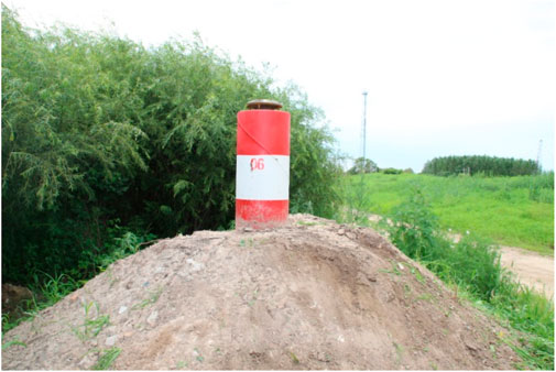
FIGURE 3. Marker-stake for surface displacement measurement.

The surface-monitoring network included 27 survey marker-stakes in the development zone and four benchmark stakes outside the development zone. The spacing between the marker-stake points was 700–1,000 m, and the stakes were more evenly arranged in the monitoring area. A Dini03 precision electronic level (Trimble, United States of America) was used to measure the height difference between two adjacent marker-stakes; the standard deviation of the round-trip measurement per kilometer was ± 0.3 mm. The marker-stakes were built in Block X of the Sazhong development zone. There are 2,499 oil and water wells in this block, covering three series of development well groups. The block area is 19.28 km², and the original formation pressure of the block is 10.13 MPa. The top depth of the oil layer is approximately 800 m, and the bottom depth is approximately 1,250 m (the total thickness of the interlayer between reservoirs is approximately 150 m). The total effective thickness of the oil layer is approximately 150 m. Figure 4 shows the locations of the marker-stakes.

FIGURE 4

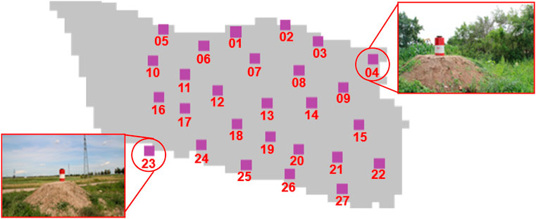
FIGURE 4. Map showing locations of the surface displacement marker-stakes.

From November 2017 to April 2018, the vertical displacement measurement of the marker-stakes and the build-up tests for the average formation pressure were conducted for Block X (Figure 4). The vertical displacement, measured twice, was the surface vertical displacement at the marker-stake locations. The surface vertical displacement field measured based on the vertical position change at two time points is shown in Figure 5.

FIGURE 5

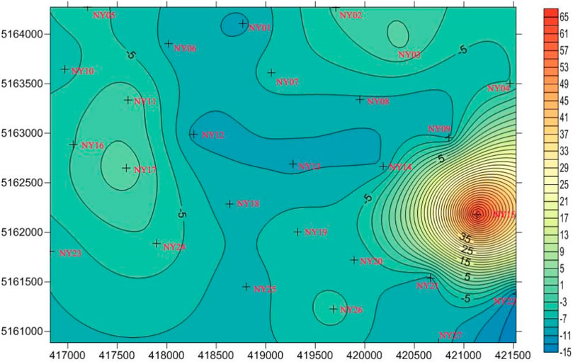
FIGURE 5. Surface vertical displacement field measured based on vertical position change from November 2017 to April 2018¹.

Because of the fewer monitoring times for formation pressure in the pressure build-up test, the grid size was expanded to 900 m × 900 m when using the formation pressure in the pressure build-up test. The change in the average pore pressure obtained from the well pressure build-up test from November 2017 to April 2018 is shown in Figure 6.

FIGURE 6

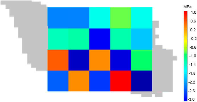
FIGURE 6. Formation pressure change from November 2017 to April 2018.

From November 2017 to April 2018, casing damage was serious in this block, and casing damage was found in most wells. At that time, it was thought that the casing damage was caused by over-high water injection amount. Therefore, hundreds of water injection wells were shut down during this period, but the oil well production was normal. Such a system leads to the decrease of injection production ratio. Because of less injection and more recovery, the average pressure of the formation decreases and the formation tends to be compacted. To measure the accuracy of the calculation results, the overall compliance degree is defined as follows:

$C=1-\frac{{\displaystyle \sum |p{\text{'}}_k-p_k|}}{{\displaystyle \sum \left|p_k\right|}}(7)$

where p'_k is the vertical displacement of the surface, as calculated based on the positive evolution at each marker-stake (mm), and p_k is the measured vertical displacement of the surface at each marker-stake (mm).

According to Eq. 7, the overall degree of compliance was 82.51%. The main reason for the error was that there were few recovered logging data, few data points to be calculated, and an excessively large grid.

The matching relationship between the change in formation pore pressure and the surface vertical displacement was investigated. Using the COMSOL finite-element software, a geomechanical model with dimensions of 10,000 m × 10,000 m × 5,000 m was established to calculate the surface displacement caused by the unit grid pressure difference, that is, the convolution kernel for the test samples. The reservoir thickness was calculated as the total thickness of the vertical sandstone of the reservoir, which was 300 m. A geometric view of the finite-element model is shown in Figure 7.

FIGURE 7

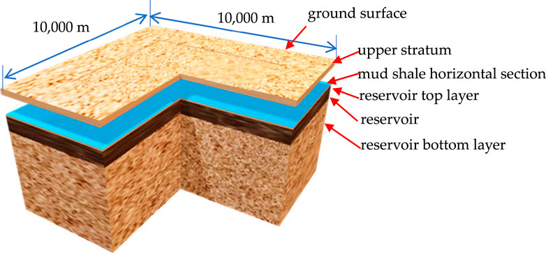
FIGURE 7. Geometric view of the finite-element model.

In the COMSOL simulation, the poroelasticity model was applied. Poroelasticity describes the interaction between fluid flow and deformation in elastic porous media like reservoir. In the poroelasticity model, the relation of stress, strain, and pore pressure is defined as:

$\mathbf{\sigma }=E\mathbf{\epsilon }-{\alpha }_{\text{B}}{p}_{\text{f}}\mathbf{I}(8)$

where σ is the Cauchy stress tensor; E is the Young’s modulus; ε is the strain tensor; α_B is the Biot coefficient, and p_f is the fluid pore pressure; I is the unit tensor.

As the change of pore pressure is not enough to make the reservoir plastic deformation, the stress-strain relationship adopts the classical linear elastic physical equation. Navier’s equations for reservoir in equilibrium under purely gravitational load is

$\nabla \cdot \mathbf{\sigma }=\left({\rho }_{\text{f}}\varphi +{\rho }_{\text{d}}\right)g(9)$

where ρ_f and ρ_d represent fluid and drained densities, respectively, and ϕ is the porosity of reservoir.

Darcy’s law is used to describe the fluid flowing in reservoir pores.

$\nabla \cdot \left({\rho }_{\text{f}}{\mathbf{u}}_{\text{f}}\right)=Q_m(10)$

${\mathbf{u}}_{\text{f}}=-\frac{K}{\mu }\left(\nabla p+{\rho }_{\text{f}}gD\right)(11)$

where u_f is the fluid velocity in reservoir; K is the permeability of the reservoir; μ is the fluid’s dynamic viscosity in reservoir; p is the fluid’s pressure; ρ_f is its density; ∇D is a unit vector in the direction over which the gravity acts.

From top to bottom, the geological model is divided into the upper stratum (700 m), mud shale horizontal section (0 m, an interface with continuous vertical displacement and discontinuous horizontal displacement), a reservoir top layer (50 m), a reservoir (300 m), and a reservoir bottom layer (3,950 m). The other parameters are listed in Table 1.

TABLE 1

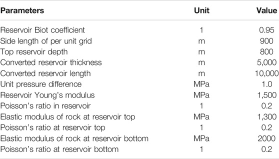
TABLE 1. Conditions and mechanical parameters of the strata in the geomechanical model.

Based on finite-element analysis, the distribution of the surface vertical displacement caused by the pressure difference in the center unit grid is shown in Figure 8.

FIGURE 8

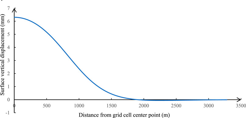
FIGURE 8. Relationship between surface displacement and pressure difference in per-unit grid.

The relationship between the surface displacement and pressure difference is represented by the convolution kernel k (x, y) for the analyzed block. For the finite element model, the surface deformation under the given pore pressure field can be calculated by changing the pore pressure of the reservoir after selecting the poroelasticity model to realize the forward calculation process. But for the inversion calculation, the software can not calculate the origin of given surface deformation, or the pore pressure field. Using the convolution neural network model in this manuscript, the inversion calculation can be realized, but a large number of forward calculation results are needed as training samples to train the convolution neural network. The forward calculation results can be got by poromechanical mechanism. The relevant part has been added in the manuscript.

Backward Evolutionary Computation Using Improved CNN Model

To compare with the average pore pressure variation from the pressure build-up test, the formation pressure dispersion of a 900 m × 900 m block was conducted. Twenty such blocks (5 in the x-direction and 4 in the y-direction) in the range of the marker-stake measurements were used for the inversion of the formation pore pressure through the vertical displacement of the surface and of the formation pore pressure obtained via the pressure build-up test. Blocks outside the range of the marker-stake measurements were not considered.

The input and output of the improved image-to-image CNN are square matrices with the same length and width. Because the boundary grid was ignored in the training of the CNN model, the input and output matrices of the model should be larger than the actual grid. In accordance with the actual conditions in Block X, a 7 × 7 input and output layer model was established.

The improved image-to-image CNN model contained 10 hidden layers. There were two channels in the first and last hidden layers and four channels in the remaining hidden layers. As the grid sizes of the input and output layers were the same, the same padding convolutional method was used to calculate the intermediate results. The convolution kernels in the CNN had a size of 3 × 3. Thus, the total number of training variables was 1,225, and the number of intermediate variables was 6,468. An activation function was not used, because a physical causal relationship exists between the formation pore pressure and surface vertical displacement. The improved image-to-image CNN model is shown in Figure 9.

FIGURE 9

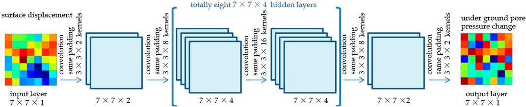
FIGURE 9. Improved image-to-image CNN model for inversion of surface vertical displacement to calculate underground pore pressure change.

The convolution kernel for forward evolution represents the surface vertical displacement field of single grid formation pore unit pressure change, and its value was obtained using the curve shown in Figure 4. In the convolution kernel, only the grids near the center possess values, and the values of the three grids outside the center are all 0. The convolution kernel size for the forward evolution was 7 × 7. The test data were obtained by assuming a pressure field and forward calculating the surface vertical displacement. Each point of the 7 × 7 formation pressure field sample randomly assumes a pressure value from −0.5 MPa to +0.5 MPa. The surface vertical displacement field was obtained via a convolution calculation using Eq. 2. We loaded eight samples at a time for training. To reduce the time cost of creating training samples, the training sample batch was changed per 20 training cycles. An adaptive moment estimation method was used to train the CNN. The same method was also used to build 64 samples for testing, and the testing samples were not used for training; they were only used to test the accuracy of the predicted pressure field. The learning efficiency was set to 0.001. The loss function only considers the error of the 5 × 5 grids in the center and not the error of the outermost grids.

We used Python 3.6 with TensorFlow 2.14 to develop an improved image-to-image CNN program. The CNN was trained 100,000 times, and the average error of the formation pressure change based on the test samples with the number of training iterations is shown in Figure 10. Figure 11 shows the formation pressure changes of the first 64 test samples compared with the prediction results of different training iterations. After 100,000 training cycles the average error of the formation pressure is 0.00495 MPa, and the formation pressure change values of each grid in the figure are not different from the real values. If the relationship between the underground pore pressure change and the surface vertical displacement measurement is completely accurate, an accurate distribution of the formation pore pressure can be obtained through the improved image-to-image CNN model.

FIGURE 10

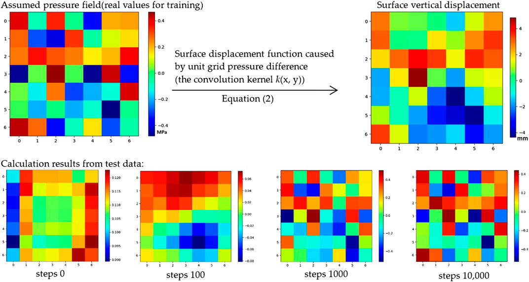
FIGURE 10. Formation pressure changes of the first sample compared with the prediction of different training iterations. In step 100,000, the formation pressure change values of each grid in the figure are not different from the real values.

FIGURE 11

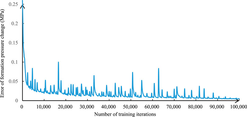
FIGURE 11. Average error of formation pressure change based on test samples with the number of training iterations.

Using the measured surface vertical displacement between November 2017 and April 2018 of Block X, we calculated the average formation pressure change of each grid within the coverage of the marker-stakes. During the period from November 2017 to April 2018, 102 wells were tested by pressure build-up test in this block, and the test was distributed in different positions in the block. The formation pressure results were averaged according to the divided in twenty 900 × 900 m blocks shown in Figure 12.

FIGURE 12

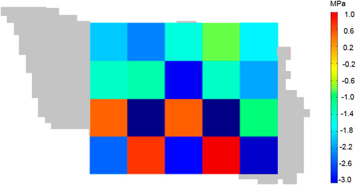
FIGURE 12. Comparison of strata pressure change from November 2017 to April 2018 from surface displacement inversion.

By comparing the average pore pressure changes shown in Figures 6, 12 in the same position, we found that the results were in good agreement; the coincidence rate of the pressure-change trend was 95%, and the overall coincidence degree was 83.12%.

The accuracy of the change in unit pressure change or convolution kernel is the most important factor affecting the final accuracy. In this method, the numerical simulation is mainly used to simulate the surface deformation field of a formation grid after changing the unit formation pressure. The surface deformation field is the convolution kernel used in forward calculation. The accuracy of the convolution kernel directly determines the prediction accuracy of the model in practical block application. There are inevitable errors in numerical simulation. One error source is the accuracy of the finite element model, which can be reduced by increasing the number of finite element meshes and optimizing the finite element model. Another error comes from the accuracy of the stratigraphic model, which can be reduced by the improvement and fine description of the block geological model. The lithology distribution and mechanical parameters of the actual strata were not the same in the plane. The discontinuous interfaces such as faults in the formation also affect the convolution kernel. These effects cause the convolution kernel to vary with the plane position. However, this effect was not considered in the present study. This is the main reason for the calculation error. Furthermore, during this period, the surface displacement increased. The basic coverage of the marker-stake measurement parameters was larger, and the measurement error was much smaller than the measurement value. In addition, the average pore pressure difference considered for the correlation was derived from the pressure build-up test. In this case, the grid area was larger, and there were only 20 grids. The amount of data used was small. Nevertheless, such data density is sufficient to meet the needs of oilfield management. The method of inversion of the average formation pore pressure via surface displacement is faster, less expensive, and more accurate.

Conclusion

(1) Surface displacement is a reflection of the formation pore pressure change. The range of formation vertical displacement due to the change in formation pore pressure is within the range of linear elastic deformation of the formation rock, and the displacement per unit grid pressure difference can be used as a convolution kernel. The distribution of the surface vertical displacement can be obtained through the convolution of the formation pore pressure and convolution kernel.

(2) Through forward evolution, the surface displacement field can be calculated using any formation pressure field. Infinite training samples can be obtained by constantly assuming the formation pressure field and calculating the corresponding surface vertical displacement.

(3) The improved CNN method adopts an image-to-image network mode instead of a pooling layer and a full connection layer. The new loss function ignores the error of the boundary grid and focuses the training of the CNN parameters on adjusting the output results. These model improvement methods effectively improved the accuracy of the model calculation.

(4) A field test in the Daqing Oilfield in China showed that the variation in the formation pore pressure obtained via inversion was 83.12%, in accordance with the results of 20 groups of pressure build-up tests within the range of marker-stake measurements. Overall, the inversion method of average formation pore pressure by surface displacement has a lower cost and is faster.

Data Availability Statement

The original contributions presented in the study are included in the article/supplementary material, further inquiries can be directed to the corresponding author.

Author Contributions

Conceptualization, CH and CA; methodology, FW and CA; validation, FW; formal analysis, CH; investigation, CH and CA; resources, CA; writing—original draft preparation, CH; writing—review and editing, FW; visualization, CH; supervision, CA.

Funding

This research was supported by National Natural Science Foundation of China (Grant No. 52074088, Grant No. 51804076). Heilongjiang Provincial Natural Science Foundation of China (Young Scientists) (Grant No. QC QC2018047).

Conflict of Interest

The authors declare that the research was conducted in the absence of any commercial or financial relationships that could be construed as a potential conflict of interest.

Publisher’s Note

All claims expressed in this article are solely those of the authors and do not necessarily represent those of their affiliated organizations, or those of the publisher, the editors and the reviewers. Any product that may be evaluated in this article, or claim that may be made by its manufacturer, is not guaranteed or endorsed by the publisher.

Footnotes

¹Measured value of Stake 15 was ignored because the stake had been damaged

References

Ai, C., Hu, C. Y., and Cui, Y. M. (2015). Casing Optimization for Delaying Casing Damage in the Datum Bed of the Daqing Oilfield. Pet. Drill. Tech. 6, 7–12. doi:10.11911/syztjs.201506002

Google Scholar

Ameh, E. G. (2019). Geochemistry and Multivariate Statistical Evaluation of Major Oxides, Trace and Rare Earth Elements in Coal Occurrences and Deposits Around Kogi East, Northern Anambra Basin, Nigeria. Int. J. Coal Sci. Technol. 6 (2), 260–273. doi:10.1007/s40789-019-0247-4

CrossRef Full Text | Google Scholar

Banik, N., Koesoemadinata, A., Wagner, C., Inyang, C., and Bui, H. T. (2013). “Predrill Pore Pressure Prediction Directly from Seismically Derived Acoustic Impedance,” in SEG Technical Program Expanded Abstracts, Houston, TX, September 2013, 2905–2909.

CrossRef Full Text | Google Scholar

Cipolla, C., Motiee, M., and Kechemir, A. (2018). “Integrating Microseismic, Geomechanics, Hydraulic Fracture Modeling, and Reservoir Simulation to Characterize Parent Well Depletion and Infill Well Performance in the Bakken,” in Paper presented at the SPE/AAPG/SEG Unconventional Resources Technology Conference, Houston, TX, July 2018. doi:10.15530/urtec-2018-2899721

CrossRef Full Text | Google Scholar

Cui, Y. M. (2015). Mechanism of Formation Slippage and Shear Casing Damage of the Marker Bed in Sazhong Development Area of Daqing Oilfield. Daqing, Heilongjiang: Northeast Petroleum University.

Dutta, N. C., and Khazanehdari, J. (2006). Estimation of Formation Fluid Pressure Using High-Resolution Velocity from Inversion of Seismic Data and a Rock Physics Model Based on Compaction and Burial Diagenesis of Shales. Lead. Edge 25 (12), 1528–1539. doi:10.1190/1.2405339

CrossRef Full Text | Google Scholar

Dutta, N. C. (2002). Deepwater Geohazard Prediction Using Prestack Inversion of Large offsetP-Wave Data and Rock Model. Lead. Edge 21 (2), 193–198. doi:10.1190/1.1452612

CrossRef Full Text | Google Scholar

Eaton, B. A. (1972). The Effect of Overburden Stress on Geopressure Prediction from Well Logs. J. Pet. Technol. 24 (8), 929–934. doi:10.2118/3719-pa

CrossRef Full Text | Google Scholar

Fillippone, W. R. (1982). “Estimation of Formation Parameters and the Prediction of Overpressures from Seismic Data,” in SEG Technical Program of Expanded Abstracts, Dallas, TX, October 1982, 482–483.

CrossRef Full Text | Google Scholar

Gao, D., Liu, Y., Guo, Z., Han, J., Lin, J., Fang, H., et al. (2018). A Study on Optimization of CBM Water Drainage by Well-Test Deconvolution in the Early Development Stage. Water 10 (7), 929. doi:10.3390/w10070929

CrossRef Full Text | Google Scholar

Guo, X., Wu, K., Killough, J., and Tang, J. (2019a). Understanding the Mechanism of Interwell Fracturing Interference with Reservoir/Geomechanics/Fracturing Modeling in Eagle Ford Shale. SPE Reservoir Eval. Eng. 22 (3), 842–860. doi:10.2118/194493-pa

CrossRef Full Text | Google Scholar

Guo, X., Wu, K., An, C., Tang, J., and Killough, J. (2019b). Numerical Investigation of Effects of Subsequent Parent-Well Injection on Interwell Fracturing Interference Using Reservoir-Geomechanics-Fracturing Modeling. SPE J. 24 (4), 1884–1902. doi:10.2118/195580-pa

CrossRef Full Text | Google Scholar

Hou, Z., Yu, H., Liu, Y., Zhang, S., and Gu, H. (2019). High-Precision Seismic Prediction of 3D Pore-Pressure in Tight Sandstone Gas Reservoirs with Low Porosity and Permeability at M Gas Field in Xihu Sag. Geol. Sci. Technol. Inf. 38 (2), 267–274. doi:10.19509/j.cnki.dzkq.2019.0232

Google Scholar

Hu, C. Y., Ai, C., and Wang, F. J. (2018). Optimization of Casing Design Parameters to Mitigate Casing Failure Caused by Formation Slippage. SDHM 2, 85–98. doi:10.3970/sdhm.2018.00115

Google Scholar

Hwang, J. K., Seo, S., Castanon, J. S., and Kim, H.-C. (2019). DFT-based Identification of Oscillation Modes from PMU Data Using an Exponential Window Function. Energies 12, 4357. doi:10.3390/en12224357

CrossRef Full Text | Google Scholar

Li, Y., Jia, D., Rui, Z., Peng, J., Fu, C., and Zhang, J. (2017). Evaluation Method of Rock Brittleness Based on Statistical Constitutive Relations for Rock Damage. J. Pet. Sci. Eng. 153, 123–132. doi:10.1016/j.petrol.2017.03.041

CrossRef Full Text | Google Scholar

Mohammady, S., Farrell, R., Malone, D., and Dooley, J. (2020). Performance Investigation of Peak Shrinking and Interpolating the PAPR Reduction Technique for LTE-Advance and 5G Signals. Information 11, 20. doi:10.3390/info11010020

CrossRef Full Text | Google Scholar

Qi, S., Zou, Y., Wu, F., Yan, C., Fan, J., Zang, M., et al. (2017). A Recognition and Geological Model of a Deep-Seated Ancient Landslide at a Reservoir under Construction. Remote Sens. 9, 383. doi:10.3390/rs9040383

CrossRef Full Text | Google Scholar

Rutqvist, J., Vasco, D. W., and Myer, L. (2010). Coupled Reservoir-Geomechanical Analysis of CO2 Injection and Ground Deformations at in Salah, Algeria. Int. J. Greenhouse Gas Control. 4, 225–230. doi:10.1016/j.ijggc.2009.10.017

CrossRef Full Text | Google Scholar

Shen, Z., Beck, F. E., and Ling, K. (2014). The Mechanism of Wellbore Weakening in Worn Casing-Cement-Formation System. J. Pet. Eng. 2014, 1–8. doi:10.1155/2014/126167

CrossRef Full Text | Google Scholar

Sheng, Y.-N., Li, W., Guan, Z.-c., Jiang, J., Lan, K., and Kong, H. (2020). Pore Pressure Prediction in Front of Drill Bit Based on Grey Prediction Theory. J. Petrol. Explor Prod. Technol. 10 (6), 2439–2446. doi:10.1007/s13202-020-00896-3

CrossRef Full Text | Google Scholar

Sun, W. L., and Sun, K. F. (2007). A Review of Seismic Formation Pressure Prediction. Prog. Explor. Geophys. 30 (6), 428–432 (In Chinese). doi:10.13809/j.cnki.cn32-1825/te.2007.06.005

Google Scholar

Tang, J., Wu, K., Li, Y., Hu, X., Liu, Q., and Ehlig-Economides, C. (2018). Numerical Investigation of the Interactions between Hydraulic Fracture and Bedding Planes with Non-Orthogonal Approach Angle. Eng. Fracture Mech. 200, 1–16. doi:10.1016/j.engfracmech.2018.07.010

CrossRef Full Text | Google Scholar

Tang, J., Fan, B., Xiao, L., Tian, S., Zhang, F., Zhang, L., Weitz, D., et al. (2021. A New Ensemble Machine Learning Framework for Searching Sweet Spots in Shale Reservoirs. SPE J. 26 (01), 482–497. doi:10.2118/204224-PA

Tipper, J. C. (1976). The Study of Geological Objects in Three Dimensions by the Computerized Reconstruction of Serial Sections. J. Geol. 84 (4), 476–484. doi:10.1086/628213

CrossRef Full Text | Google Scholar

Wang, X., and Sheng, J. J. (2018). A Self-Similar Analytical Solution of Spontaneous and Forced Imbibition in Porous media. Adv. Geo-energy Res. 2 (3), 260–268. doi:10.26804/ager.2018.03.04

CrossRef Full Text | Google Scholar

Wei, M. A., Chen, C., Wang, Y. J., and Ma, H. (2007). New Approach for Pore Pressure Prediction. Oil& Gas Geol. 28 (3), 395–400. (In Chinese). doi:10.3321/j.issn:0253-9985.2007.03.014

Google Scholar

Xie, J., Tang, J., Yong, R., Fan, Y., Zuo, L., Chen, X., et al. (2020). A 3-D Hydraulic Fracture Propagation Model Applied for Shale Gas Reservoirs with Multiple Bedding Planes. Eng. Fract. Mech. 228, 106872. doi:10.1016/j.engfracmech.2020.106872

CrossRef Full Text | Google Scholar

Xiong, X. J., Huang, J., Chen, R., Liao, Y., and Yuan, Y. (2019). Pore Pressure Prediction Method of Under-compacted Formation. Comput. Tech. Geophys. Geochem. Explor. 41 (1), 1–5. doi:10.3969/j.issn.1001-1749.2019.01.001

Google Scholar

Xu, W., Liu, R., Yang, H., Zhang, L., and Yang, Y. (2019). “Investigation of Well Testing Reservoirs with Multiphase Flow in a Mature Field,” in SIMULATION: Transactions of the Society for Modeling and Simulation International. doi:10.1155/2019/2847345

CrossRef Full Text | Google Scholar

Xu, X.-q., and Zhou, H.-b. (2019). Study on the Influence of Pulse Current Cathodic Protection Parameters of Oil Well Casing. Adv. Mater. Sci. Eng. 2019, 1–9. doi:10.1155/2019/2847345

CrossRef Full Text | Google Scholar

Xue, D., Zhou, J., Liu, Y., and Zhang, S. (2018). A Strain-Based Percolation Model and Triaxial Tests to Investigate the Evolution of Permeability and Critical Dilatancy Behavior of Coal. Processes 6, 127. doi:10.3390/pr6080127

CrossRef Full Text | Google Scholar

Yu, F., Jin, Y., Chen, M., Lu, Y. H., Niu, C. C., and Ge, W. F. (2014). Discussion on a Formation Pore Pressure Detection Method for Carbonate Rocks Based on the Thin Plate Theory. Pet. Drill. Tech. (5), 57–61. doi:10.11911/syztjs.201405010

Google Scholar

Yun, M. H. (1996). Formation Pressure Prediction Using Seismic Data. Oil Geophys. Prospect. 31 (4), 575–586. (In Chinese).

Google Scholar

Zhang, Q., Li, X., Bai, B., Hu, S., and Shi, L. (2018). Effect of Pore Fluid Pressure on the Normal Deformation of a Matched Granite Joint. Processes 6, 107. doi:10.3390/pr6080107

CrossRef Full Text | Google Scholar

Zhang, F., An, M., Zhang, L., Fang, Y., and Elsworth, D. (2020). Effect of Mineralogy on Friction-Dilation Relationships for Simulated Faults: Implications for Permeability Evolution in Caprock Faults. Geosci. Front. 11 (2), 439–450. doi:10.1016/j.gsf.2019.05.014

CrossRef Full Text | Google Scholar

Zhang, J., Li, Y., Pan, Y., Wang, X., Yan, M., Shi, X., et al. (2021). Experiments and Analysis on the Influence of Multiple Closed Cemented Natural Fractures on Hydraulic Fracture Propagation in a Tight Sandstone Reservoir. Eng. Geol. 281, 105981. doi:10.1016/j.enggeo.2020.105981

CrossRef Full Text | Google Scholar

Zhao, X., Zhou, L., Pu, X., Jin, F., Shi, Z., Han, W., et al. (2020). Formation Conditions and Enrichment Model of Retained Petroleum in Lacustrine Shale: A Case Study of the Paleogene in Huanghua Depression, Bohai Bay Basin, China. Pet. Explor. Dev. 47 (5), 916–930. doi:10.1016/s1876-3804(20)60106-9

CrossRef Full Text | Google Scholar