 Christoph Mayer*
 Carlo Licciulli
- Bavarian Academy of Sciences and Humanities, Geodesy and Glaciology, Munich, Germany
It can easily be expected that debris-covered glaciers show a different response on external forcing compared to clean-surface glaciers. The supra-glacial debris cover acts as an additional transfer layer for the energy exchange between atmosphere and ice. The related glacier reaction is the integral of local effects, which changes strongly between enhanced melt for thin debris layers and considerably reduced melt for thicker debris. Therefore, a realistic feedback study can only be performed, if both the ice flow and the debris-influenced melt is treated with a high degree of detail. We couple a full Stokes representation of ice dynamics and the most complete description of energy transfer through the debris layer, in order to describe the long-term glacier reaction in the coupled system. With this setup, we can show that steady-state conditions are highly unlikely for glaciers, in case debris is not unloaded from the surface. For continuous and complete debris removal from the lowermost glacier tongue, however, a balance of the debris budget and the glacier conditions are possible. Depending on displacement and removal processes, our results demonstrate that debris-covered glaciers have an inherent tendency to switch to an oscillating state. Then, glacier mass balance and debris balance are out of phase, such that glacier advance periods end with the separation of the heavily debris-loaded lowermost glacier tongue, at time scales of decades to centuries. As these oscillations are inherent and happen without any variations in climatic forcing, it is difficult to interpret modern observations on the fluctuation of debris-covered glaciers on the basis of a changing climate only.
1 Introduction
The knowledge about debris-covered glaciers advanced considerably during the last two decades. This development was driven by the recognition that debris-covered glaciers represent considerable parts of the cryosphere in many mountain regions, especially in High Mountain Asia (HMA), but also other mountain ranges.
Especially three features of debris-covered glaciers came into the focus of scientific investigations: the effect of debris thickness and other inherent parameters on melt rates, the distribution of debris cover across individual glaciers and glaciated mountain ranges and the different morphological expressions of debris-covered glaciers like ice cliffs, melt ponds and surface debris redistribution. The effect of debris cover on the glacier evolution, however, attracted much less attention, even though the interaction between a surface mass balance influenced debris cover and ice dynamics fundamentally determines the extent and distribution of debris-covered glaciers. Here we introduce four key papers, in order to demonstrate some important issues in the development of modelling debris-covered glaciers.
A first numerical description of a coupled ice/debris glacier system was presented by Konrad and Humphrey (2000). They used a simplified force balance approach with shear stress as the single driver for describing ice dynamics along a two-dimensional (2-D) flow line, assuming parallel ice flow and a constant surface slope of the glacier. Debris input was prescribed as constant and restricted to the ELA, while debris transport was solely through downward advection of ice. However, the additional effect of the debris load on the shear stress was accounted for. Their linear mass balance function was affected by the existence of surface debris, which reduces ice melt exponentially to the respective debris thickness. This model predicts an infinite glacier length for steady-state conditions. Higher debris input leads to a thinner mean debris layer, due to an increase in ice velocity, while a steepening of the mass balance gradient leads to lower ice thicknesses, because the higher mass transport reduces debris thickness and thus increases ice melt. However, the limitations of the model (constant surface slope, simple mass balance parameterisation, singular debris source) only allow very general conclusions.
In a more practical approach, Rowan et al. (2015) used a higher-order shallow-ice (SIA) model, including longitudinal and transverse stress gradients, as well as a simple description of basal sliding to simulate the evolution of debris-covered Khumbu Glacier in the Himalaya. The effect of debris on ice melt was described by an exponential function, which reduces ablation from the clean-ice value to 50% at 0.5 m debris thickness and prescribes diminishing ablation rates for debris thicknesses exceeding 1 m. Debris is transported from the accumulation region (with a constant input concentration) by advection along flow paths to either the surface or the bed (in case of basal melting) in the ablation zone. Simulations were initialised for Late Holocene conditions in order to reconstruct a steady-state maximum extent. This served as a base for investigating the glacier evolution towards its present state and into the future, where the elevation of the ELA was the climatic driver. Experiments for clean-ice conditions and reduced ice melt resulted in a present glacier extent much smaller than currently observed (16% of the modern volume for the clean-ice case) compared to the existence of glacial debris. The results demonstrate that only the implementation of debris-related processes enable reliable simulations of debris-covered glaciers and support the observations that mass loss at such glaciers is mainly by surface lowering compared to frontal ice melt.
A further development was made by Anderson and Anderson (2016), who also used a 2-D numerical flow line model (SIA, coupled with longitudinal stress gradients) to investigate the role of englacial and supraglacial advection of debris and its impact on the mass balance for glacier evolution. They used a hypothetical clean-ice steady state on a linear bed as initial condition and perturbing it with step functions of debris deposition. The prescribed altitudinal mass balance gradient is modified by the effect of the debris cover, which assumes a hyperbolic decline of ice melt with debris thickness, neglecting enhanced ice melt for very thin debris cover. Debris loss occurs by introducing a terminal wedge, which allows the definition of a discharge debris flux. All experiments were driven to a steady state, where the integrated glacier mass balance disappeared and a balance was reached between debris deposition and debris loss from the terminus. It appeared that the final glacier length strongly depends on the magnitude of debris deposition and the relation between melt rate and debris thickness. Also, the location of debris deposition strongly influences the glacier geometry, because a deposition near the ELA has a more sustained effect on the mass balance. The observation of a reduced AAR for debris-covered glaciers in comparison with clean-ice glaciers could be confirmed by these experiments.
Ferguson and Vieli (2021) extended these investigations with the aim of defining the role of the debris cover on the glaciers transient behaviour, but also analysed the effect of cryokarst features in such a system. The methods are strongly based on Anderson and Anderson (2016), but now include the formation of supra-glacial lakes and ice cliffs for a stagnant glacier tongue. Debris concentration is uniform in the glacier and thus ice melt produces a constant contribution of supra-glacial debris. The existence of supra-glacial debris reduces ice melt according to an inverse relationship with debris thickness (Nicholson and Benn, 2006). Debris slides off the terminus if a threshold ice thickness is reached, resulting in a permanent exposition of ice at a frontal cliff. With this configuration, the authors are capable of simulating steady states, where surface mass balance and debris balance are both zero. Based on these conditions, the effect of a changing climate on the glacier evolution is investigated by abrupt changes as well as introducing white noise on the changes. They found that debris cover influences the geometric evolution of glaciers and especially the length response to warming periods is delayed. This characteristic is mitigated by contrasting melt enhancement, if cryokarst features are included in the simulations.
These examples demonstrate that the general feedback mechanisms of glacial debris can be reproduced by using simplified ice-dynamics models, coupled with a debris model of varying complexity. We also do not aim on explaining the full dynamic response of debris-covered glaciers. In particular, we do not delve into details like cryokarst phenomena or variability of englacial debris distribution, even though this likely has relevant consequences on the general glacier evolution (e.g., Wirbel et al. (2018), Miles et al. (2021)). We rather want to point out some crucial fundamental conditions, which might help to understand the complex behaviour of such glaciers. Therefore, we first raise the well-known question about the steady state of debris-covered glaciers, which seems straightforward but turned out to be rather complex. Then, we investigate the problem of debris unloading at the glacier terminus, which turns out to be crucial when it comes to potential steady-state conditions. Finally, we investigate the possibility of recurring glacier advances due to a hysteresis in the ice flux—ice melt balance of the glacier terminus.
Our experiments are based on two sophisticated models, which apply extensive physical theories to ice melt under a debris cover (Evatt et al., 2015) and the detailed evolution of glacier geometry by solving the full Stokes equations for ice deformation using Elmer/Ice (Gagliardini et al., 2013). In doing so, we ensure that the complex relation between debris thickness and ice melt is represented across the entire thickness scale based on physical principles, including enhanced melt rates for thin debris layers in the upper part of the ablation region. Considering that we simulate small-scale glaciers, the full Stokes approach ensures that we can rely on a most realistic geometry of the glacier terminus and frontal dynamics, which is crucial for our debris discharge experiments and evolution of the whole system.
2 Model Description
2.1 Surface Mass Balance
Ice melt beneath a supra-glacial debris cover is rather complex, due to the interaction of different energy fluxes and the usually inhomogeneous composition of the debris column. The first issue can be tackled by applying a sophisticated physical model, which includes all important fluxes. The highly variable structure of the debris layer is rather location dependent and cannot be solved in detail for larger areas, because of unknown initial conditions and rather random variability in debris composition (e.g., Nicholson et al., 2018; Fyffe et al., 2020). However, for our application the assumption of homogeneous conditions is justified, because we focus on long-term and general glacier evolution, not aiming on resolving localised melt variability. Therefore, we decided to use an ablation model, which is capable of describing the melt rate for all debris thicknesses by including turbulent fluxes within the upper debris cover (Evatt et al., 2015). This formulation resolves the enhanced melt rates for a thin debris cover as well as the decreasing melt rates for thickening debris above a threshold of typically less than 10 cm (e.g., Östrem, 1959; Nicholson and Benn, 2006). As forcing, we use artificial and constant climate conditions, which are based on annual mean values of the required variables in dependence of altitudinal gradients (see the selected parameter set in Supplementary Table S1). Thus, we simulate a climate, which enables the existence of glaciers and their steady state in the model domain, comparable to alpine conditions with glaciers of several kilometers in length, extending across an elevation range between 2,800 m and 3,500 m. Figure 1 shows an example of the surface mass balance model in case of a clean-ice and a debris-covered glacier simulation.
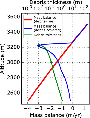
FIGURE 1. Mass balance gradient used in the basic experiments for clean-ice conditions (red) compared with an example mass balance gradient from a debris-covered glacier (blue). The green curve indicates the corresponding example debris thickness profile.
2.2 Ice Dynamics
The key goal is to investigate the effect of debris cover on glacier dynamics, which we approach by deploying a full Stokes flow-line model. The gravity-driven ice flow is solved by considering momentum balance and mass conservation. We treat ice as an incompressible fluid with constant density ρice = 910kg m−3 and assume viscous flow according to Glen’s law with exponent n = 3 to relate deviatoric stresses and strain (Greve and Blatter, 2009). Since we focus on the effect of debris cover on glacier evolution, we switch off englacial thermodynamical processes and assume constant climate forcing. The temperature dependent flow rate factor A(T) is kept constant and derived from an Arrhenius-type law (Cuffey and Paterson, 2010) with pre-exponential factor A0 = 1.916 × 10³s−1 Pa−3, activation energy Q = 139 kJ mol−1 K−1 and a constant englacial temperature, set to T = –3°C.
The coupling between the debris layer and the underlying ice is twofold. Debris coverage has an effect on the glacier flow via its strong influence on the surface mass balance. This, in turn, influences the debris distribution itself, since debris transport depends on the flow field. In our modelling approach we simplify these feedback mechanisms. In particular we did not consider 1) the change in the momentum balance due to additional debris-induced stress on the ice surface and 2) the effect of englacial debris on the rheology of the debris/ice mixture. Further, the exclusion of englacial thermodynamical processes implies that 3) we do not capture temperature changes within the glacier derived from the debris-perturbed surface thermal boundary condition. These simplifications, however, do not compromise the suitability of our model setup to investigate the fundamental dynamical behaviour of debris-covered glaciers, because we do not expect these processes to considerably alter the basic feedback mechanisms.
The modelled ice/debris glacier system is forced by changes in surface mass balance in response to the evolving debris coverage, despite the constant climatic boundary condition at the debris/ice surface and thus a constant clean-ice surface mass balance distribution (Figure 1). The resulting glacier geometry variations are governed by the free-surface equation (Greve and Blatter, 2009), which calculates surface elevation changes due to down-slope transport of ice and local mass balance. Moreover, we investigate the response of the system to different basal sliding conditions. We calculate basal flow velocities using a simple linear relation between the basal velocity component parallel to the bedrock vb∥ and the corresponding basal stress component τb∥:
where β2 is the friction coefficient. The basal velocity component perpendicular to the bedrock is set to zero (vb⊥ = 0) in order to avoid ice penetration into the bedrock. For the simulations without basal sliding, the entire basal velocity vector is set to zero (no-slip condition).
2.2.1 Debris Source and Transport
Debris is generally deposited on glaciers due to avalanches or rockfalls, but it can also be incorporated in the ice column by lateral or basal erosion (Wirbel et al., 2018). If this happens in the accumulation zone, debris submerges into the ice, is transported within the ice body and re-emerges in the ablation zone. There, debris remains on the glacier surface and is transported passively down-valley towards the terminus (neglecting any redistribution processes). Even though several studies (e.g., Miles et al., 2021; Wirbel et al., 2018) demonstrate the importance of spatial variations of englacial debris concentration, we do not include processes for debris input to the glacier, nor debris transport within the ice. Although the variability in such processes certainly influences the glacier reaction on the climatic boundary conditions, we focus on the fundamental debris-glacier-climate feedback at the glacier surface. Therefore, we only consider an englacial debris concentration ζ which is constant in time and space, as a result from debris deposition and transport. Based on the analysis of ice flux gradients in our experiments, we consider this constraint as a further but potentially minor limitation of the coupling between debris cover and glacier dynamics, since extensive or compressive flow will not alter the debris concentration before emergence. We define ζ as the ratio between the height of the debris column within the debris/ice mixture and the total height of the debris/ice mixture and use different prescribed debris concentrations to explore its influence on the glacier dynamics.
In the modelling approach, debris is only considered, if it emerges at the glacier surface. As this is only the case for melt conditions, a supra-glacial debris cover is limited to the ablation zone. Therefore, an emerging debris height dD results from ice melt
The newly emerged debris dD is added to the already existing local debris height D.
The debris layer is transported with the ice flow downstream towards the glacier terminus. This debris advection is governed by the calculated surface flow field and therefore includes compressive or extensive flow and thus dynamic thickening or thinning of the debris cover. We calculate debris advection only at the glacier surface, which reduces the problem in our 2-D glacier geometry to a 1-D advection problem. The advection of the debris column D by a known 1-D velocity (i.e., the horizontal surface velocity component vx) is:
where Ds is the debris source from melting ice, which is calculated by integrating Eq. 2.
2.2.2 Debris Displacement and Removal
A major issue in investigating long-term glacier evolution is related to the fate of supra-glacial debris, when it reaches the glacier terminus, because melt conditions at the lowermost part of the glacier are crucial for the dynamics of the whole system. At least for debris covers of several tens of centimeters (which is usually the case for well developed debris covered glaciers), debris loss by completely melting the underlying ice is very small compared to downstream debris transport rates. Thus, any substantial debris removal from the glacier requires an active process. The observational basis for developing appropriate mechanisms is weak and theoretical approaches are few (Moore, 2018). We do not aim on providing an elaborated theory about debris mobilisation and removal from the terminus. We rather established some very simple algorithms, which mimic complicated debris migration processes in a general way and thus allow us to investigate the glacier response.
One way to deal with the debris layer on the terminus is to consider only the surface velocity field and neglect any active debris migration. Because the ice velocity approaches zero at the terminus, supra-glacial debris will then accumulate to very large and finally unrealistic debris thicknesses. In reality, it is reasonable that in presence of steep slopes, as it is often the case at the glacier front, single rocks are mobilised or an entire debris layer may abruptly slide down, and thus leave the system. We implemented mechanisms in the model, which lead to displacement or removal of debris. These mechanisms can be switched on separately or in a combined form, allowing us to investigate the consequences in detail.
Purely slope-triggered removal sets in, where the slope of the ice surface exceeds a prescribed threshold
where ρd is the density of the bulk debris layer (i.e., accounting for porosity in the layer), g the gravitational acceleration, D the thickness of the debris layer and α the surface slope. If the driving stress exceeds a defined yield stress
In addition to these complete removal conditions, we also implemented algorithms to describe step-wise gravitational debris displacement along the glacier surface in the terminus area. This mechanism resembles slumping of parts of the debris layer along steep ice slopes and can involve the whole debris column or a fraction f only. This approach is motivated by observations of sediment flow on glaciers (Lawson, 1982), but is parameterised in a more general fashion as a partial failure due to a slope dependent instability. The fraction of displaced debris is linearly dependent on the surface slope α. Moreover, displacement sets in only if the surface is steeper than a threshold slope αt, while f is defined as:
where M and C are arbitrary parameters. Eq. 5 ensures that f is constrained within the interval [0, 1] and is valid in case αt < (1 − C)/M. For αt ≥ (1 − C)/M, Eq. 5 reduces to a step function of αt, where the entire debris column is removed for surface slopes above the threshold. Note that the surface slope α in Eq. 5 must be expressed in terms of surface gradient (not in percentage and not in degree).
Tumbling of rocks and thus granular movement of the debris column depends on several contingencies, like e.g., the shape of single rocks and the meter-scale topography of the debris layer. Therefore, as an alternative to the deterministic calculation of f, the model contains also a stochastic approach. In this case f is a random number, which is uniformly distributed within the slope-dependent interval (αM + C − δ, αM + C + δ), where δ is an arbitrary parameter. We also ensure for the stochastic approach that f is within the interval [0, 1] deploying a formulation that is analogous to Eq. 5.
2.3 Numerical Implementation
The numerical model is implemented using the finite-element software package Elmer/Ice (Gagliardini et al., 2013). The ice-flow component of the model is based on established tools and is briefly described in section 2.3.1. On the other side, all debris-related components are completely new and are described in more detail in section 2.3.2. The basic modelling approach is illustrated in Figure 2, whereas a more detailed schematic overview is provided in Figure 3.
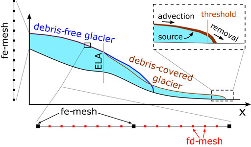
FIGURE 2. Ice/debris glacier system as implemented in our modelling approach. The bedrock geometry is pre-defined, while glacier evolution is determined by external forcing. Debris emerges below the ELA in consequence of ice melt and is advected down-valley. Different mechanisms determine the fate of terminal debris. Ice dynamics is calculated on an fe-mesh (black squares), whereas debris advection requires a finer fd-mesh (red squares).
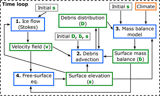
FIGURE 3. Schematic representation of our modelling approach. Blue boxes indicate essential equations (with order of execution). Important state variables are in green. Grey boxes indicate variables requiring an initialisation. Climate forcing is kept constant (orange box).
2.3.1 Stokes Flow
We solve the Stokes equations on a 2-D flow line geometry and use a synthetic bedrock topography, which is inclined at higher altitudes and rather flat in the lower part (see Figure 4). This is the only geometrical input of the model, representing a mountain slope with a horizontal length of 4.5 km. The finite-element mesh was generated using gmsh (Geuzaine and Remacle, 2009). We opted for a structured mesh with quadrilateral elements. The mesh has a horizontal resolution of 10 m and it counts eleven evenly-distributed layers in the vertical direction. All simulations run with a time step of one year, which implies that all involved physical quantities (e.g., mass balance) are yearly-averaged quantities.
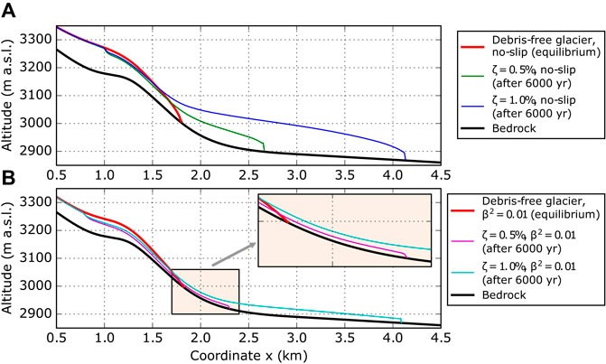
FIGURE 4. Modelled evolution of glacier geometry for clean and debris-covered glaciers in case of (A) no-slip and (B) sliding conditions at the glacier base. Clean-ice equilibrium states (red) are compared with debris-covered states after 6,000 years (not in equilibrium). Glaciers with higher debris concentration (ζ = 1.0%) are longer (blue and cyan). On the other side, basal sliding reduces the mean glacier thickness (magenta and cyan).
Using the finite-element method reduces the solution of the Stokes system to a linear system. We tackle this, deploying the direct Unsymmetric-pattern MultiFrontal method for sparse systems (UMFPACK; Davis, 2004), which ensures robustness to the solving procedure. For solving the free-surface equation we use the BiConjugate GradientStabilised method (BiCGStab; Kelley, 1995) and apply transient stabilisation (Akin and Tezduyar, 2004), which is necessary to smooth the glacier front and avoid that the ice piles up instead of advancing. Stability of the simulations is improved by adding an artificial ice layer of thickness Hmin to ice-free bedrock areas (Wirbel and Jarosch, 2020).
2.3.2 Debris Advection
Obtaining stable solutions of the advection equation requires, in general, higher grid resolution and shorter time steps (Courant et al., 1928), compared to the Stokes system. On the other hand, the single solution of the Stokes system is computationally much more expensive compared to the advection equation. We calculate debris advection within the finite-element frame of Elmer/Ice. In contrast to the main simulation, advection is solved on a 1-D finite-differences scheme with an ad-hoc finer mesh (fd-mesh) and shorter time step. This approach proved to be very convenient, as it combines stability and computational efficiency. We refine the finite-element mesh (fe-mesh) by inserting equi-distributed sub-nodes (see Figure 2). If the fe-mesh has N nodes and grid size ΔX, the fd-mesh has n = (N − 1) × (r + 1) + 1 sub-nodes and sub-grid size Δx = ΔX/(r + 1), where r is the refinement factor, i.e., the number of sub-nodes between two nodes of the fe-mesh. Similarly, the reduced time step size Δt is a fraction of the original time step size ΔT, such that Δt = ΔT/s (both r and s are integers).
We discretise the advection equation using an upwind scheme, where derivatives are calculated considering sub-nodal values in the direction of the flow origin. This approach avoids oscillations in the advected debris distribution:
where i is the sub-node index and j the time sub-step index. Debris source Ds is added to the existing debris coverage before the advection step (i.e., not after each time sub-step). Fe- and fd-mesh communicate via shared nodes. Each (r + 1)th sub-node coincides with an fe-mesh node and all fe-nodes are shared nodes. Sub-grid variables required to solve Eq. 6 (e.g., ice velocity) are linearly interpolated between nodal values of the fe-mesh. After completing all time sub-steps within a main time step, the advected debris distribution is communicated to the fe-mesh. This happens by copying shared sub-nodal values to the fe-mesh. All sub-nodal debris values (shared and non-shared) are not modified by the Stokes solver and are used as initial condition for the next advection step (after adding again Ds from the mass balance equation).
Solving the advection equation according to Eq. 6 is not volume-conserving. Therefore, we calculate the volume integral over the whole debris layer before and after the advection step. The ratio ψa between the two integrals quantifies the artificial debris volume change due to the applied solution scheme. We multiply the whole debris distribution by ψa, in order to compensate for this artifact.
In addition, Eq. 6 produces small artificial changes in the spatial distribution of the advected scalar quantity, which are superimposed to real changes due to gradients in the advection velocity. In particular, it tends to flatten edges and adds long and thin tails at the downstream end of the advected distribution. These artifacts have, in general, only a small influence on the model evolution. However, in our study, these thin tails impact the simulation results, since thin debris layers create the highest ice ablation (see section 2.1 and Figure 1). We tackle this issue by cutting off those tails (i.e., setting them to zero debris thickness) at the node (fe-mesh), where debris thickness is less than 0.1 m and less than 50% of the previous (uphill) node. Sub-nodal values uphill from the first adjusted node are not modified, in order not to alter the successive advection step. This procedure works, since the thickness of the debris coverage steadily increases down-valley and rapidly drops only at the glacier terminus, where the tails occur. We compensate the debris losses due to this correction by applying a scaling factor ψt to the remaining advection distribution, which is analogous to the previously introduced factor ψa.
Our model does not include periglacial moraine mechanics for debris migration and generation of terminal moraines, as this is far out of scope of this paper. Therefore, debris deposited on bedrock after a frontal retreat is completely removed. If the glacier retreats and ice thickness drops below
2.3.3 Model Structure
We simulate the ice/debris glacier system combining the governing equations described above as shown in Figure 3. First we deploy the Stokes solver to calculate the ice velocity field according to the current glacier geometry (i.e., provided as initial condition or from the previous time step). The velocity field together with information about the current debris distribution, surface mass balance (required to determine the debris source term) and surface topography (needed for debris displacement and removal mechanisms, if active) is used to solve the advection equation on the fd-mesh and determine the new debris distribution. After returning to the fe-mesh, the new debris distribution is used to calculate the new mass balance profile. This, together with the velocity field, is used by the free-surface equation to calculate surface evolution, which is the starting point for the next time iteration.
3 Description of Experiments
Even though the effect of debris cover on ice melt is investigated in high detail on a large number of glaciers, it is difficult to relate this local information to the general glacier evolution. Also, exploiting satellite imagery gives only a rather limited insight into the ongoing changes, because the evolution of debris-covered glaciers covers a much larger time scale then the satellite era. Therefore, the application of suitable models is required to shed light on the fundamental and long term glacier behaviour.
In order to investigate the general feedback mechanisms, we run a suite of experiments with different, but temporally constant englacial debris concentrations and various debris unloading schemes, as well as for different basal conditions. The bandwidth of parameter variations should provide a broad coverage of potential glacier configurations and thus allow insight into the general evolution characteristics of debris-covered glaciers. An overview of all performed simulation runs is given in Table 1.
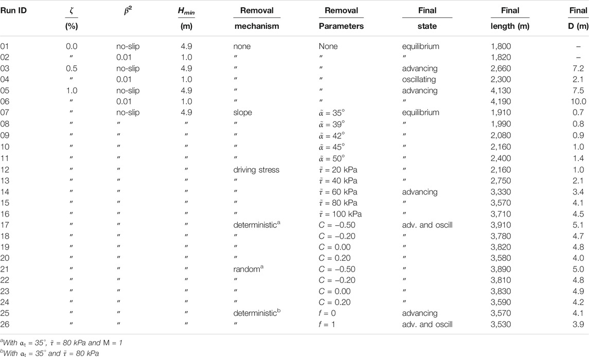
TABLE 1. Overview of performed simulations. Runs with debris-free glaciers (ID 01 and 02) end when the glaciers reach steady state. All other simulations run for 6,000 years. The last three columns report glacier states after those simulation times. Non-equilibrium states may change running the model over longer time periods.
We decided to run the experiments for a maximum of 6,000 years, because our results show that this time is sufficient for the glaciers to show their characteristic dynamical behaviour. It turned out that changes over the final 1,000 years of the 6,000 years simulation period are small and do not alter characteristic variables significantly (if we consider e.g., advancing rates or oscillation periods).
3.1 Experiments Without Gravitational Removal of Debris
One of the principal questions about debris-covered glaciers is concerning the potential existence of steady state, despite a continuous supply of debris to the glacier surface by melt out (Anderson and Anderson, 2016; Ferguson and Vieli, 2021). For the sake of simplicity, we assume an englacial debris concentration, which is constant in space and time, because we are interested in the basic glacier feedback, not in specific scenarios. Ice flux in the ablation zone generally decreases towards low values along the flow of a glacier, equalling surface ablation at the snout in the case of steady state. If debris piles up on the glacier terminus over time (due to compressive flow and melt out), melt rates approach zero and so does also ice flux. This results in negligible horizontal transport of supra-glacial debris, which prohibits debris transport across the terminus (if no gravitational removal is allowed) and leads to debris accumulation in the terminus region and thus a further reduction in melt. As a consequence, the mass balance turns positive and ice flux leads to a glacier advance and thus increases the ablation region. As long as debris is not removed from the glacier surface, this feedback will lead to a continuous length growth in the model, while on a real glacier differential melt and dirty-ice areas at the margin of the debris cover might change its geometry and thus also mobilisation of debris (Fyffe et al., 2020). To investigate this hypothesis of indefinite glacier growth for accumulating debris, we run a sequence of experiments with different, but temporally constant englacial debris concentrations. We expect the results to provide insight into the temporal evolution, characteristic time scales and a potential approximation of steady conditions of a debris-covered glacier in the case of no debris loss from the glacier front. These experiments are partly motivated by the observation of debris-covered and more or less stagnant glacier termini, which lack any evidence of widespread debris removal (e.g., Baltoro Glacier in the Karakoram, Inylcheck Glacier in the Tian Shan).
3.1.1 The Effect of Different Debris Concentrations
Englacial debris concentration probably has a strong influence on the time scales of glacier evolution, because the melt out of englacial debris directly influences the surface mass balance conditions. Therefore, we test this influence by running otherwise identical setups with englacial debris concentrations of ζ = 0.5% and 1.0%. These values represent a reasonable range compared to recent in-situ observations at a heavily debris-covered glacier (Miles et al., 2021). All simulations start from the same steady-state debris-free geometry, which is reached by applying the surface mass balance conditions described in the model setup (see section 2.1 and Supplementary Table S1) to our standard bedrock geometry until a constant clean-glacier volume is reached. Debris advection is calculated on an fd-grid setting r = 7 and s = 10 (see section 2.3.2). The amount of emerging debris for each grid cell results directly from the ice melt. The artificial debris mass loss, connected to the advection algorithm, is quantified and compensated. Also, the thin debris tail at the downstream end of the advected debris distribution is removed and the mass loss compensated. The minimum ice thickness is set to Hmin = 4.9 m. In case of a retreating glacier front, all debris located downstream of the terminus (first sub-node with ice thickness below Hmin down-glacier from the equilibrium line) is removed from the system. This is a considerable simplification compared to real conditions, because periglacial moraine deposits probably influence the dynamics of a recurrent glacier advance. However, taking into account such deposits (and developing a suitable deformation model) would have complicated the numerical setup too much, without providing essential insight due to the poor knowledge of the required physics.
3.1.2 The Effect of Basal Sliding
The above described experiments are performed under conditions of a frozen bed. Basal sliding has an important impact on the glacier evolution and very likely many of the debris-covered glaciers show temperate conditions at least below the equilibrium line. The investigation of glacier reaction for different basal conditions aims mainly on the time scales involved and the differences in glacier geometry in the context of debris cover and debris accumulation. Therefore, the same experiments as above are conducted with the sliding parameter β2 set to 0.01 (see Eq. 1). The initial state of the simulations is a debris-free equilibrium state calculated setting β2 = 0.01 as well. Compared to the no-slip case, switching on sliding results in higher flow velocities, lower ice thickness, but similar glacier lengths. Because of the reduced glacier thickness, we reduce the minimum ice thickness to Hmin = 1 m.
3.2 Experiments With Gravitational Removal of Debris
The above condition of indefinite debris accumulation only serves as an idealised fundamental feedback system of debris-covered glaciers. The more realistic case is a removal of debris from the glacier terminus in one or another way. Here, we investigate the consequences of several basic mechanisms of debris removal on glacier response. The experiments are conducted on glaciers with englacial debris concentration ζ = 1.0% and no-slip basal conditions.
3.2.1 Abrupt Removal
First we implement the abrupt removal of debris after reaching a defined threshold at a specific location (see section 2.2.2). Debris downstream of this location is entirely removed. The threshold can be a critical surface slope
3.2.2 Continuous Debris Displacement and Abrupt Removal
Instead of an instantaneous complete removal of debris from the terminus, it often can be observed that supra-glacial debris slides down steep slopes in a more continuous way, if the slope is not too steep. We maintain an abrupt removal mechanism (for a yield stress of
4 Results
4.1 Equilibrium State of the Clean-Ice Case
First, we present model runs for clean-ice conditions, which we further use as initial state for all subsequent experiments with englacial debris concentrations. Due to the constant climate forcing, the model reached steady-state conditions for both no-slip and basal sliding conditions. With the chosen bedrock topography and the prescribed surface mass balance (indeed the calculated surface mass balance changes according to variations in surface elevation), the glacier developed from ice-free conditions and equilibrium was reached after 600 years for the no-slip case. Based on this state, and switching on basal sliding results in additional ca. 200 years to reach a new equilibrium state for β2 = 0.1 and another 200 years to reach equilibrium with β2 = 0.01. The model results show almost the same final glacier length of about 1.8 km (see Figure 4). However, the ice thickness distribution is rather different. The no-slip glacier shows a maximum ice thickness of about 95 m almost exactly half-way downstream, while for the sliding case the maximum results to about 63 m at the same distance (see Supplementary Figure S1). As a consequence, the surface elevation is more than 30 m lower in the region of the equilibrium line for sliding conditions, while the 2-D “volume” is about 30% smaller. Also the glacier velocities are considerably different, with a vertically-averaged horizontal velocity maximum of 10 m/yr for the sliding case and 5.5 m/yr for the no-slip case, respectively (Supplementary Figure S2). Due to the bedrock geometry, the maximum ice velocities are observed a few hundred meters downstream of the equilibrium line.
4.2 Equilibrium-State Experiments Without Debris Removal
The initial motivation for these experiments was to test the hypothesis that debris-covered glaciers cannot reach or approximate a steady state if the emerging debris remains on the glacier. In the case of close-to-balanced conditions, the unloading of debris might be difficult, because of vanishing ice velocities at the front.
Figure 4 shows glacier geometries for debris concentrations of ζ = 0.5% and 1.0% and different basal conditions spanning 6,000 years of evolution. Starting from a debris-free glacier, the increasing debris cover protects the underlying ice and the glaciers start to advance. The growth of the glacier depends on the debris concentration and results in a more than doubled glacier length and an increase of the glacier volume by over 150% for a debris concentration of 1.0%. In case of smaller englacial debris concentrations, glacier length and volume changes are more moderate, indicating convergence to conditions of clean-ice glaciers.
Basal conditions do not significantly influence the glacier length, but have a strong impact on the glacier thickness. Compared to the initial debris-free geometry, ice thicknesses just downstream of the equilibrium line reduce in the case of basal sliding by about 15–20 m (Supplementary Figure S1) and this thinning extends further upstream across the equilibrium line. The lower parts of the glaciers beyond the clean-ice terminus are also thinner in case of sliding, with thicknesses reduced by 60–75% compared to the no-sliding case (about 25 m compared to about 90 m for ζ = 1.0%). This also leads to a migration of the equilibrium line of about 200 m further upstream and a reduction of the accumulation area by about 20%.
Maximum ablation rates are observed just downstream of the equilibrium line with values exceeding −3 m/yr, while ablation approaches zero towards the terminus, in accordance with the expected effect of the varying debris thicknesses. Higher flow velocities due to sliding enlarge the size of the thin-debris and high-melt area (see Supplementary Figures S3, S4). This effect leads to a stronger reduction of ice volume for sliding conditions, but also increases the melt-out rate of englacial debris. After 6,000 years of model evolution we observe a mean debris thickness of 10 m in case of basal sliding and 7.5 m for the corresponding no-slip experiment for ζ = 1.0%, while unrealistic values of almost 40 m of debris are reached close to the terminus. The change to ζ = 0.5% reduces the mean debris thickness to 7.2 m (see Table 1).
All simulations without debris removal show an ongoing glacier advance even after 6,000 years evolution, except for the ζ = 0.5% sliding case (Figure 5). The glacier advance in case of ζ = 1.0% and basal sliding conditions is faster compared to the no-slip case for the first few millennia. However, after 5,500 years, the non-sliding glacier surpasses the sliding glacier in length, indicating a stronger imbalance compared to the sliding case. However, none of the experiments seem to approach steady-state conditions.
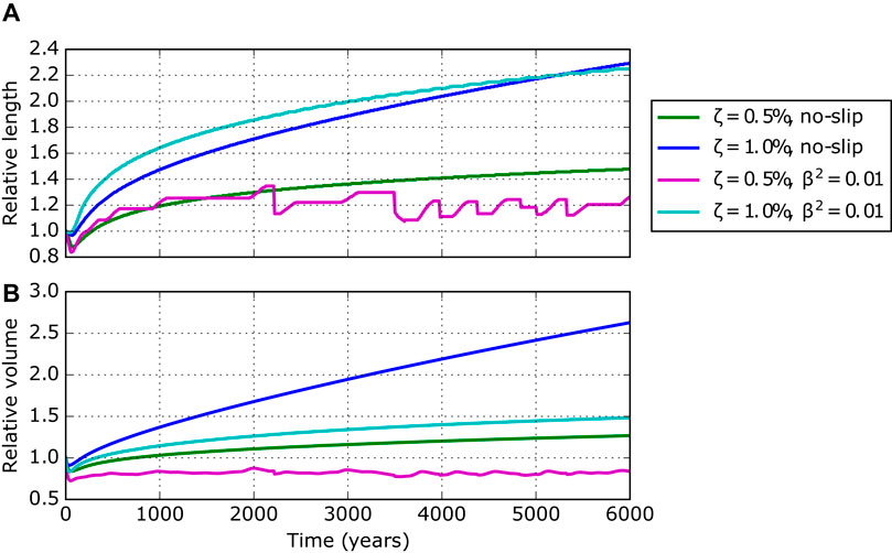
FIGURE 5. (A) Glacier length and (B) volume evolution of simulated debris-covered glaciers for different englacial debris concentrations (ζ = 0.5% and 1.0%) and different basal conditions (no-slip or sliding with β2 = 0.01). Lengths and volumes are relative to the corresponding clean-ice equilibrium state. After 6,000 years evolution none of the systems is in equilibrium. The system with ζ = 0.5% and β2 = 0.01 (magenta) is in an erratically oscillating state. The other three systems are in an advancing state.
The experiment with ζ = 0.5% and sliding conditions is characterised by erratic length oscillations with amplitudes of a few hundred meters. The model approaches repeatedly a close-to-balance state, but collapses afterwards. Figures 6 and 7 illustrates details of such a cycle (for further details on the debris budget see Supplementary Figure S5A). First, the glacier advances as in the other experiments (green profile in Figure 7). However, due to a continuous slow down across the glacier tongue, ice loss by ablation surpasses mass gain from ice flux (see red areas in Figure 6, e.g., at t ≈ 2,100 years). This imbalance results in a slow reduction of ice thickness (blue profile in Figure 7), which intensifies towards the equilibrium line with its thinner debris cover. The surface slope of the glacier tongue flattens even more and ice flux decreases further (cyan profile). Finally, the lower tongue separates from the main glacier within about a century (magenta profile) and the mass balance of the remaining glacier (15% shorter) turns positive, leading to an advance of the new terminus. The cyclicity in our experiments ranges from a few centuries up to about 1,000 years. During such periods the remaining dead-ice body with about 10 m depth will disappear even for rather small ablations rates before the re-advancing glacier will cover it. Periods of close-to-balance conditions last up to 1,000 years. However, the red stripes in Figure 6 (e.g., between t = 1,000 and 2,000 years) indicate that the glacier undergoes dynamical changes, despite the constant length and apparent quiescence. Regions with net mass loss are evident, but the imbalance is not strong enough to trigger a separation and the ice column above the low-flux area thickens and adjusts the flux budget.
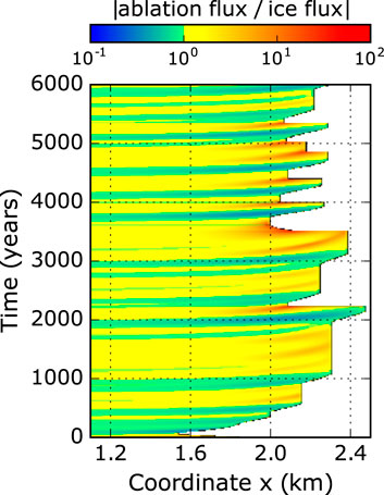
FIGURE 6. Evolution of the ratio between ablation flux and ice flux for the oscillating experiment (magenta curve in Figure 5) with ζ = 0.5% and β2 =0.01, calculated at each node. The ablation flux results from integrating from the current node to the downstream end of the glacier. The ice flux is calculated by integrating the ice flow through a vertical line at the current node. The ratio increases when the glacier advances, due to an increase of the ablation area. A clear divergence is evident at locations where the glacier collapses. The collapse reduces the length of the ablation area, which results in values of the flux ratio below one (green to blue), which initiates a new advance phase.
FIGURE 7. Illustration of glacier conditions for the erratic oscillation state of the glacier system with ζ = 0.5% and β2 = 0.01. Four typical phases are captured: frontal advance (green), further frontal advance and thinning in the low-flux area (blue), glacier state just before the collapse (cyan), new geometry just after the collapse (magenta).
These results indicate that glaciers will not reach a final steady state for the chosen boundary conditions. The glaciers rather continue to advance or turn into an oscillating state with a periodicity of several centuries and up to millennia. By extending the simulation time to more than 6,000 years, it is an open question whether the glaciers would approach steady state, keep growing or advance until detaching the frontal part and enter an oscillating state. However, such time scales of at least several millennia exceed most evolution scales of mountain glaciers anyway.
4.3 Equilibrium-State Experiments With Debris Removal
The experiments with a continuous accumulation of supra-glacial debris already demonstrate that this condition is not realistic for large time scales. Even though, some glaciers like e. g. Baltoro Glacier show very stable frontal conditions with no obvious debris transport into the flood plain, for more than a century. But also here some debris is removed at the basal water outlet through slumping from the steep cliff above. In the case of a steep glacier front and/or a thick frontal debris layer, the loss of debris from the glacier system is very likely. Our experiments for slope-only and driving stress induced debris mobilisation (see section 2.2.2) will investigate possible glacier reactions to such processes. In these experiments, debris at the glacier front is removed from the system as soon as the threshold conditions are met, resulting in a clean-ice glacier front which adapts its geometry to the prevalent melting conditions. Supra-glacial debris, which is advected across the upstream boundary of this region, is again removed, if the glacier geometry still meets the threshold conditions. The same is valid for emerging debris, which reaches the surface of the glacier front in consequence of ice melt.
Glacier length in these experiments with complete debris removal depends strongly on either of the parameters
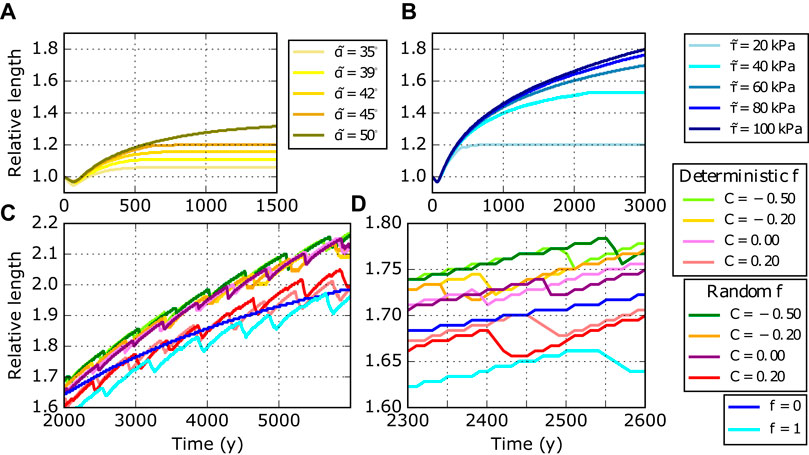
FIGURE 8. Glacier length evolution for different debris removal and displacement mechanisms. (A) Slope-triggered debris removal; (B) driving-stress triggered debris removal; (C) deterministic and random slope-induced debris displacement combined with abrupt driving-stress triggered debris removal. Panel (D) is a zoom of (C). Whereas in (A) and (B) the glaciers can reach steady state if
A more episodic debris transport across the glacier front, where only a certain proportion of the debris is completely removed is probably the more realistic case. The supra-glacial debris column at the unstable node is distributed across the neighboring downstream nodes in dependence of the frontal slope, before it finally leaves the system. This condition resembles a glacier front with different slope angles, where parts of the glacier front are ice-free, while neighboring regions still are debris-covered and changing surface angles will continuously modify the debris cover. The corresponding experiments reveal that a steady state is not established under such conditions.
The amount of transient supra-glacial debris on the glacier front depends on the parameter C in Eq.5. Figure 8C shows the effect of C on the temporal evolution of debris-covered glaciers (see Figure 8D for a zoomed view of Figure 8C). We test C in the range −0.50 to 0.20. The resulting differences are small between using the deterministic and the random mechanism. For lower (negative) C, the fraction f of displaced debris (we always set M = 1) becomes smaller and vice versa. If f = 0, debris displacement is zero and the simulation reduces to the example with
Within the simulation period of 6,000 years the glaciers advance and are far from steady state, although the rate of growth decreases with time. The growth is periodically interrupted by short retreat periods (ca. every 500 years). These phases last a few decades and result in glacier length reduction of some tens of meters. Figure 9 reveals details of those oscillations in case C = 0.20 (further details in Supplementary Figure S5B). Since f is close to one, the fraction of displaced debris is large and nodes become almost debris-free, as soon as surface slope exceeds αt. The high melt rates influence the slope of the glacier front, which is lowered below αt. Because of the less inclined front, a thicker frontal debris layer is required to exceed
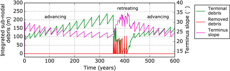
FIGURE 9. Evolution of debris coverage and slope of the terminus in case of deterministic debris displacement and removal for C = 0.20. Terminal debris is the sum of sub-nodal debris loads across the last five nodes (green). Removed debris is calculated from sub-nodal values as well (red). Terminus slope is calculated considering the last five nodes (magenta). Note that the last five nodes migrate in flow direction in case of an advancing glacier. Just after advancing to the next node, the last glacier node has very low debris cover and surface elevation. This bias is responsible for the observed saw tooth behavior.
The main difference between experiments with debris displacement and experiments with debris removal without displacement is the steeper slope of the terminus in the latter case. Unloading events are therefore more frequent, but the amount of removed debris is small. It follows that the induced imbalance is moderate. It can be promptly compensated by the ice flux from above and by the formation of a new debris layer. The imbalance is too gentle to generate visible length oscillations. It remains an open question whether the combination of debris displacement and removal could stop glacier growth after 6,000 years simulation time and whether the glaciers would enter an oscillating state.
5 Discussion
We tried to design simple experiments, which nevertheless represent characteristic settings of debris-covered glaciers and thus form the basis for investigating fundamental glacier reactions. We did not intend to simulate all complex feedback mechanisms, which would just distract from the principal relationships between mass balance, debris cover and ice dynamics. However, we used a full Stokes model and small grid dimensions in order to obtain a realistic glacier geometry as far as possible. Another difference to earlier studies is the implementation of enhanced met rates for thin debris covers combined with a more physically based melt function.
Based on simple mass conservation considerations it seems obvious, that debris-covered glaciers cannot reach a steady state, unless the accumulated volume of supra-glacial debris on the glacier tongue also is in equilibrium with the melt-out conditions. Konrad and Humphrey (2000) argued that a debris-covered glacier in steady state must be infinitely long. This is in principle true: if debris is not allowed to leave the system, it accumulates and reduces ablation at the terminus almost to zero. Still, continuous glacier volume growth is expected in case of ongoing accumulation of supra-glacial debris on the glacier tongue, even though the growth rates monotonically approach zero. However, our experiments indicate that the time scales under such conditions are in the order of centuries to millennia even for moderate glacier sizes (see e.g., the example with ζ = 0.5% and without sliding in Figure 5). A comparable glacier evolution in the real world will be strongly superposed by climatic fluctuations, which are not included in our experiments. But even by including glacier response to moderate climate variations, it might be impossible to discriminate between close-to-steady conditions under the dominating climate and minimal growth rates due to long-term debris accumulation. A glacier with a moderate mean englacial debris concentration (ζ ≈ 0.5%) can therefore evolve over many centuries in a rather continuous way with only small debris accumulation rates on the lower tongue, adding up to several meters in total debris thickness. During the usual observation intervals of a few years up to some decades, no significant change in glacier geometry will be observed for such glaciers, while climate sensitivity will be greatly reduced over the centuries, due to the build-up of a thick debris cover on the lower terminus.
However, it is clear that an indefinite growth of debris thickness is impossible and certain removal mechanisms gain importance over time. Our results show that, without unloading mechanisms, the debris coverage of the lowermost glacier tongue may reach unrealistic values of up to 40 m (see Supplementary Figure S3, S4). Recent studies introduced debris down-wasting mechanisms to overcome this apparent unrealistic behavior of indefinite glacier growth. Anderson and Anderson (2016) implemented a triangular terminal wedge parameterisation, which enables debris flux into the foreland and provides conditions for the glacier to reach steady state. Ferguson and Vieli (2021) followed a more pragmatic approach, removing debris if the ice thickness falls below a critical value. This condition permits the glacier to reach steady state as well. Those simplified approaches reflect a different focus of those studies with respect to ours, aiming on more general conclusions.
One possibility of overcoming the problem of continuous glacier growth results from the inversion of the vertical mass balance gradient in the case of debris-covered glaciers (see Figure 1), which shows decidedly higher melt rates towards the equilibrium line compared to the lower glacier tongue. This strong gradient leads to a reduction in surface slope across the glacier tongue over time (see Figure 4), because of the higher melt rates upstream. In consequence, the mass flux through the tongue will be reduced.
The simulation run with englacial debris concentration ζ = 0.5% and basal sliding conditions shows that the feedback between reduced flux and high melt rates can potentially lead to a separation of the lower tongue from the main glacier. If this happens, the loss of a considerable part of the ablation zone (ca. 25%) and a subsequent accumulation of supra-glacial debris on the new terminus leads to a new advance of the remaining glacier. The dead ice body very likely melts down, before being covered by the advancing ice. This cyclic behaviour is only evident in the experiment with basal sliding and low debris concentration, because glaciers with basal sliding conditions are thinner and more likely to collapse. Moreover, they have shorter reaction times, such that temporary flux imbalances turn into rapid geometry changes, which can enforce the imbalance and induce a collapse.
We are aware that very thick debris columns might compromise our assumption about the additional debris-induced stress on the ice surface, which we neglect in the momentum balance. Including the weight of the debris layer in the momentum balance will have an impact on the dynamics of the system similar to enhanced sliding and thus enforce the oscillation mechanism to a small degree.
The glacier separations of our idealised setup are difficult to observe in nature, because natural climate fluctuations, the non-continuous englacial debris concentration and additional processes of debris redistribution and melt hot spots on the glacier tongue likely modify the evolution of the modelled cycles. On the other hand, observed elevated glacier beds with clearly expressed lateral and terminal moraines, where frontal debris cannot easily be transported off the glacier (e.g., Khumbu Glacier, Ngozumpa Glacier, Nepal) might be the result of subsequent terminus collapses in the past.
Our simulations show that glacier oscillations are suppressed, if we increase the englacial debris concentration ζ to 1.0% or impose no-slip basal conditions (both changes modify the glacier states towards less ablation and larger ice volumes). In these cases the generated glacier systems advance over the whole simulation period of 6,000 years. We do not know how the glaciers would behave, if we would further extend the simulation in time: they could keep growing, reach a steady state (at least asymptotically) or enter an oscillating state. The glacier system with ζ = 0.5% and no-slip conditions and the system with ζ = 1.0% and β2 = 0.01 show very small growth rates at the end of the simulation time. This indicates close-to-balance conditions, but on time scales in the order of millennia.
In the view of a dynamic debris budget, Anderson and Anderson (2016) broadly investigated consequences of varying the location of debris input in the accumulation area and considered englacial debris transport. Ferguson and Vieli (2021) explored the effect of debris coverage on glacier response time in reaction to climatic variation. Our investigation of different debris discharge mechanisms in relation to the question about the steady state of debris-covered glaciers is connected to the conceptual examination given in Konrad and Humphrey (2000) relative to debris-induced terminus dynamics. In particular, the authors considered an advancing terminus with debris resting on top of the ice, which is exposed to high ablation rates on the clean down-glacier side. The enhanced melt lowers the terminus surface, which becomes steeper. Debris starts ravelling down the face of the glacier and accumulates at the base. Piled debris protects the advancing ice face, which overrides the fallen debris. Debris removal mechanisms that we implemented shed light on Konrad and Humphrey (2000)’s conceptual model. However, two major issues still hamper its full numerical realisation: 1) the realistic representation of terminus geometry evolution; 2) modelling debris pile-up at the base of the ice front and the overriding of the debris pile. The first issue requires careful treatment of the surface evolution. In case of an advancing glacier front, we observe that the calculated free surface is characterised by small irregularities in the terminus region (see the little spikes just above the steep glacier fronts in Figure 4, e.g., green profile). Wirbel and Jarosch (2020) pointed out similar instability issues in case of inequality-constrained free-surface evolution and showed that full Stokes representations of glacier dynamics are able to reproduce realistic geometries, when treating the free-surface problem with appropriate stabilisation techniques. In our case, instabilities are minor and appear in experiments without debris removal, where front advance is fast and the terminus geometry is not decisive for the glacier evolution, because it doesn’t govern the debris mass balance. We are therefore convinced that the observed minor numerical instabilities at the glacier front do not impact our results. On the other hand, off-glacier debris dynamics and the overriding of periglacial deposits could be tackled with additional physics. However, the coupling with the frontal glacier dynamics is not yet solved.
Episodic or continuous removal of frontal debris depositions is a pre-requisite for a long-lasting debris balance. Otherwise the accumulation of debris in front of the glacier will prevent further debris migration from the glacier. Therefore, either melt water events, erosion by river flow or other processes need to remove the unloaded debris from the region in front of the glacier terminus. An equilibrium between debris melt out and its removal can likely be established, if such external conditions exist. This might then lead to a steady-state glacier geometry in case of constant climate conditions. We only focused on the on-glacier processes and glacier length under such conditions depends on the critical surface angle for debris migration or the related critical stress conditions. The glaciers then reach equilibrium states with lengths of up to 1.5 times the clean-ice glacier equilibrium length, which is 1.8 km in our model setup. For critical driving stresses between 60 and 100 kPa the observed length increase is up to 105% after 6,000 years simulation. Those are non-equilibrium states, but it is likely that a balanced state would be reached, running the simulation over longer time periods.
Because such an ongoing complete debris removal across the entire frontal zone is not realistic, we also investigated continuous debris displacement mechanisms combined with removal events. Under such conditions, the glacier shows a cyclic behaviour, which is superimposed to a general advancing trend (see Figure 8C). The retreating phases are short (few decades), of small amplitude (less than 50 m) and occur every ca. 500 years. Small fluctuations of debris-covered glaciers, which are observed today (e.g., Scherler et al. (2011), Banerjee and Shankar (2013)), therefore, could result from the complicated interaction between ice and debris dynamics, decoupled from the climatic superposition.
Excluding the question about steady state, fundamental results of our investigation are consistent with previous modelling studies, where comparable. We observe that debris input increases the glacier length and reduces the AAR. Moreover, as pointed out in Anderson and Anderson (2016), when approaching the terminus, the presence of debris coverage reduces gradients of thickness, surface velocity and ice flux (see Supplementary Figures S1, S2). As in Ferguson and Vieli (2021), we could validate that the debris layer delays the glacier length response with respect to the volume response, especially in the retreating case. We observe this e. g. in the experiment without debris removal with oscillations (ζ = 1.0% and β2 = 0.01) where, after reaching the maximum extension, volume loss sets in, before the glacier length starts decreasing (see Figures 5, 6). The retreat is massive, only after the collapse of the stagnant terminus. Our results show that debris-covered glaciers quickly converge to steady state, if debris is allowed to leave the system. In particular (as Anderson and Anderson (2016) also show), a faster unloading mechanism and thus lower thresholds
6 Conclusions
The existence of supra-glacial debris considerably complicates the energy exchange between glaciers and the atmosphere. Several additional physical processes play a role and, together with the wide range of debris properties, makes it unlikely, that ice ablation can be calculated on a local scale across extended glacier regions. Furthermore, the feedback mechanisms between ice dynamics, debris dynamics and surface energy balance influence and might obscure the glacier reaction to climatic variations. Therefore, we focused this study on the relation between the glacier response on debris thickness variations only and used an appropriate numerical setup to ensure the most realistic dynamic glacier response. Our results show that the glacier-debris interaction leads to long periods of adaptation, which can reach even millennia also for medium-sized glaciers. Therefore, the glaciers’ climate response can be superposed by the ongoing adaptation to the changing debris cover on any time scale.
Moreover, we demonstrated that debris-covered glaciers have an inherent ability to shed supra-glacial debris by separating the highly debris-covered tongue region from the main glacier in case of continuous accumulation of debris. As a consequence, the glacier loses a part of its volume and the changed mass balance conditions initiate a subsequent glacier advance. If debris on the lowermost tongue is directly removed, the glacier develops a steady state, depending on the continuity and conditions of the debris removal. Given that all arriving debris is continuously and fully expelled from the glacier, it is possible to reach a balance between debris melt-out and removal. In consequence, such a system also develops a steady state with regard to the ice mass balance. However, such a continuous and complete debris removal, without any modifying effect on the exposed ice areas at the terminus, is not realistic. A more transient debris evacuation, where debris displacement on the glacier surface (without leaving the glacier system) is allowed, leads again to an oscillating reaction of the glacier, where debris balance and ice balance are slightly shifted in time. For our chosen model setup, these oscillations are superimposed to a predominant advancing phase: periods of few hundred years with ca. 100 m length increase (for our setup) and short retreating phases of few decades, where the glaciers lose tens of meters of length.
Our parameterisations of the physical processes of debris evacuation are rather simple, but demonstrate that debris-covered glaciers will show inherent fluctuations on a broad time scale even without changes in the forcing. In a next step it is necessary to work on a more accurate treatment of the dominating processes, including a more advanced representation of glacier fronts and a proper description of periglacial debris dynamics. This also includes the implementation of debris load in glacier dynamics, which might affect regions with very thick debris cover and small ice thicknesses. Such experiments will provide important details about the periodicity and the magnitude of the glacier response. In addition, the interaction between climate variations and the inherent glacier-debris response needs to be investigated, in order to reveal potential feed-back reactions, which determine the ongoing and future glacier evolution. However, even our basic experiments demonstrate, that the evolution of debris-covered glaciers under a changing climate very likely are underlain by long-periodic responses to the glacial debris mass budget, which complicate the interpretation of the climatic impact.
Data Availability Statement
The original contributions presented in the study are publicly available. This data can be found here: https://github.com/carlolic/DebrisExp. Further inquiries can be directed to the corresponding author.
Author Contributions
CM designed the study. CL conducted the numerical experiments. Both authors wrote the manuscript.
Funding
This research was funded by institutional funding of the Bavarian Academy of Sciences and Humanities.
Conflict of Interest
The authors declare that the research was conducted in the absence of any commercial or financial relationships that could be construed as a potential conflict of interest.
Publisher’s Note
All claims expressed in this article are solely those of the authors and do not necessarily represent those of their affiliated organizations, or those of the publisher, the editors and the reviewers. Any product that may be evaluated in this article, or claim that may be made by its manufacturer, is not guaranteed or endorsed by the publisher.
Acknowledgments
We highly appreciate the thorough reviews by LA and PM, which helped to improve the manuscript.
Supplementary Material
The Supplementary Material for this article can be found online at: https://www.frontiersin.org/articles/10.3389/feart.2021.710276/full#supplementary-material
References
Akin, J. E., and Tezduyar, T. E. (2004). Calculation of the Advective Limit of the SUPG Stabilization Parameter for Linear and Higher-Order Elements. Comput. Methods Appl. Mech. Eng. 193, 1909–1922. doi:10.1016/j.cma.2003.12.050
Anderson, L. S., and Anderson, R. S. (2016). Modeling Debris-Covered Glaciers: Response to Steady Debris Deposition. Cryosphere 10, 1105–1124. doi:10.5194/tc-10-1105-2016
Banerjee, A., and Shankar, R. (2013). On the Response of Himalayan Glaciers to Climate Change. J. Glaciol. 59, 480–490. doi:10.3189/2013jog12j130
Courant, R., Friedrichs, K., and Lewy, H. (1928). Uber die partiellen Differenzengleichungen der mathematischen Physik. Math. Ann. 100, 32–74. doi:10.1007/bf01448839
Cuffey, K. M., and Paterson, W. S. B. (2010). The Physics of Glaciers. 4th Edition. Cambridge, Massachussetts, US: Academic Press.
Davis, T. A. (2004). A Column Pre-ordering Strategy for the Unsymmetric-Pattern Multifrontal Method. ACM Trans. Math. Softw. 30, 165–195. doi:10.1145/992200.992205
Evatt, G. W., Abrahams, I. D., Heil, M., Mayer, C., Kingslake, J., Mitchell, S. L., et al. (2015). Glacial Melt under a Porous Debris Layer. J. Glaciol. 61, 825–836. doi:10.3189/2015jog14j235
Ferguson, J. C., and Vieli, A. (2021). Modelling Steady States and the Transient Response of Debris-Covered Glaciers. Cryosphere 15, 3377–3399. doi:10.5194/tc-15-3377-2021
Fyffe, C. L., Woodget, A. S., Kirkbride, M. P., Deline, P., Westoby, M. J., and Brock, B. W. (2020). Processes at the Margins of Supraglacial Debris Cover: Quantifying Dirty Ice Ablation and Debris Redistribution. Earth Surf. Process. Landforms 45, 2272–2290. doi:10.1002/esp.4879
Gagliardini, O., Zwinger, T., Gillet-Chaulet, F., Durand, G., Favier, L., de Fleurian, B., et al. (2013). Capabilities and Performance of Elmer/Ice, a New-Generation Ice Sheet Model. Geosci. Model. Dev. 6, 1299–1318. doi:10.5194/gmd-6-1299-2013
Geuzaine, C., and Remacle, J.-F. (2009). Gmsh: A 3-D Finite Element Mesh Generator with Built-In Pre- and post-processing Facilities. Int. J. Numer. Meth. Engng. 79, 1309–1331. doi:10.1002/nme.2579
Greve, R., and Blatter, H. (2009). Dynamics of Ice Sheets and Glaciers. Springer, Dordrecht, Heidelberg, London. New York. Science & Business Media. doi:10.1007/978-3-642-03415-2
Konrad, S. K., and Humphrey, N. F. (2000). Steady-state Flow Model of Debris-Covered Glaciers (Rock Glaciers). Wallingford:Iahs Publication, 255–266.
Lawson, D. E. (1982). Mobilization, Movement and Deposition of Active Subaerial Sediment Flows, Matanuska Glacier, alaska. J. Geol. 90, 279–300. doi:10.1086/628680
Mamot, P., Weber, S., Schröder, T., and Krautblatter, M. (2018). A Temperature- and Stress-Controlled Failure Criterion for Ice-Filled Permafrost Rock Joints. Cryosphere 12, 3333–3353. doi:10.5194/tc-12-3333-2018
Miles, K. E., Hubbard, B., Miles, E. S., Quincey, D. J., Rowan, A. V., Kirkbride, M., et al. (2021). Continuous Borehole Optical Televiewing Reveals Variable Englacial Debris Concentrations at Khumbu Glacier, nepal. Commun. Earth Environ. 2, 1–9. doi:10.1038/s43247-020-00070-x
Moore, P. L. (2018). Stability of Supraglacial Debris. Earth Surf. Process. Landforms 43, 285–297. doi:10.1002/esp.4244
Nicholson, L., and Benn, D. I. (2006). Calculating Ice Melt beneath a Debris Layer Using Meteorological Data. J. Glaciol. 52, 463–470. doi:10.3189/172756506781828584
Nicholson, L. I., McCarthy, M., Pritchard, H. D., and Willis, I. (2018). Supraglacial Debris Thickness Variability: Impact on Ablation and Relation to Terrain Properties. Cryosphere 12, 3719–3734. doi:10.5194/tc-12-3719-2018
östrem, G. (1959). Ice Melting under a Thin Layer of Moraine, and the Existence of Ice Cores in Moraine Ridges. Geografiska Annaler 41, 228–230. doi:10.1080/20014422.1959.11907953
Rowan, A. V., Egholm, D. L., Quincey, D. J., and Glasser, N. F. (2015). Modelling the Feedbacks between Mass Balance, Ice Flow and Debris Transport to Predict the Response to Climate Change of Debris-Covered Glaciers in the Himalaya. Earth Planet. Sci. Lett. 430, 427–438. doi:10.1016/j.epsl.2015.09.004
Scherler, D., Bookhagen, B., and Strecker, M. R. (2011). Spatially Variable Response of Himalayan Glaciers to Climate Change Affected by Debris Cover. Nat. Geosci. 4, 156–159. doi:10.1038/ngeo1068
Wirbel, A., and Jarosch, A. H. (2020). Inequality-constrained Free-Surface Evolution in a Full Stokes Ice Flow Model (Evolve_glacier v1.1). Geosci. Model. Dev. 13, 6425–6445. doi:10.5194/gmd-13-6425-2020
Keywords: glacier dynamics, debris cover, steady state, glacier-debris feedback, long-term glacier evolution
Citation: Mayer C and Licciulli C (2021) The Concept of Steady State, Cyclicity and Debris Unloading of Debris-Covered Glaciers. Front. Earth Sci. 9:710276. doi: 10.3389/feart.2021.710276
Received: 15 May 2021; Accepted: 16 September 2021;
Published: 14 October 2021.
Edited by:
Koji Fujita, Nagoya University, JapanReviewed by:
Leif S. Anderson, The University of Utah, United StatesPeter Moore, Iowa State University, United States
Copyright © 2021 Mayer and Licciulli. This is an open-access article distributed under the terms of the Creative Commons Attribution License (CC BY). The use, distribution or reproduction in other forums is permitted, provided the original author(s) and the copyright owner(s) are credited and that the original publication in this journal is cited, in accordance with accepted academic practice. No use, distribution or reproduction is permitted which does not comply with these terms.
*Correspondence: Christoph Mayer, Y2hyaXN0b3BoLm1heWVyQGtlZy5iYWR3LmRl