Submarine Groundwater Discharge From Sediments and Sand Boils Quantified by the Mean Residence Time of a Tracer Injection

To quantify submarine groundwater discharge, we developed an inexpensive automated seepage meter that applies a tracer injection and the computation of the mean residence time. The SGD-MRT is designed to measure a wide range of discharge rates from about 30 to 800 cm³/min and allows minimizing backpressures caused by pipe friction or flow sensors. By modifying the inner volume of the flow-through unit, the range of measurement is adjustable to lower or higher discharge rates. For process control and data acquisition, an Arduino controller board is used. In addition, components like temperature, conductivity, and pressure sensors or pumps extend the scope of the seepage meter. During field tests in the Wadden Sea, covering tidal cycles, discharge rates of more than 700 cm³/min were released from sand boils. Based on the measured discharge rates and numerical integration of the time series data, a water volume of about 400 dm³ with a seawater content of less than 12% was released from the sand boil within 7 h.

Introduction

The release of fresh or brackish waters from sediments, karst channels, or pockmarks into bottom waters has been reported for numerous coastal regions, river beds, or lakes (Zektzer et al., 1973; Lee, 1977; Bokuniewicz, 1980; Cherkauer and McBride, 1988; Moore, 1996; Burnett et al., 2003; Rosenberry, 2008; Judd and Hovland 2009; Povinec et al., 2012). Submarine groundwater discharge (SGD) flows through the pore space of sediments or along fluid conduits such as karst structures. The relevance of SGD for the transport and release of nutrients, trace elements or gases such as methane or radon from sediments into the groundwater of coastal regions or lakes has already been emphasized by Johannes (1980), Zimmermann et al. (1985), Shaw and Prepas (1990), Simmons (1992) and Bugna et al. (1996).

In order to quantify fluid discharge from the seafloor, the calculation of radon or radium budgets in the water column, pore water studies, different types of flow sensors, or seepage meters are applied (Taniguchi and Fukuo, 1993; Vanek 1993; Moore, 1999; Burnett et al., 2006; Rocha et al., 2009; Santos et al., 2009).

According to the broad range of flow rates, different sediment types, or modes of fluid transport like the dispersed flow-through permeable sediments or the focused flow along conduits, various methods and flow sensors are used to quantify fluid discharge (Sholkovitz et al., 2003; Martin et al., 2004; Schlüter et al., 2004; Seeberg-Elverfeldt et al., 2005; Koopmans and Berg, 2011; Solomon et al., 2020). Overviews of different types of flow meters for quantifying fluid discharge from sediments are provided by Taniguchi et al. (2019), Rosenberry et al. (2020), and Duque et al. (2020).

Most of these flow sensors primarily develop to quantify volume flows of fluids in technical or industrial applications such as domestic water treatment, food industry, process engineering, or the chemical industry. For such applications, mechanical or electronic feedback loops are used to regulate pressure changes and flow rates caused by narrow cross-sections or bottlenecks within flow meters, pipes, or valves.

In contrast to confined flow, under free surface flow conditions such as SGD, the flow patterns and flow lines in porous sediments or karst structures can change when the backpressure exceeds certain thresholds. This might cause shifts in flow lines and changes in discharge rates. Such effects have been demonstrated – for example – by Murdoch and Kelly (2003) and Cable et al. (2006).

We observed the effect of backpressure on measured discharge rates while using a Lee-type chamber (L 30 × W 30 × H 12 cm) equipped with an impeller flow sensor on the Sahlenburg mudflat (Figure 1A). About 2 h after the deployment of the seepage meter, the fluid discharge at the sampling site significantly decreased, and a new discharge site with intensive fluid release built up about 40 cm aside from the primary discharge site (Figure 1B). The relocation of the subsurface water transport from B1 to B2 and the formation of a new active sand boil mainly result from the backpressure created by the impeller flow sensor deployed at site B1. This observation underlines the need to minimize flow resistance when measuring fluid discharges from sediments.

FIGURE 1

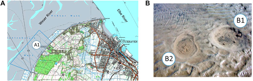
FIGURE 1. Study area (A) in the Elbe-Wester estuary in the southeastern North Sea, where groundwater discharge is observed in numerous places in the Sahlenburg mudflat (A1). (https://nibis.lbeg.de/cardomap3/?TH=534). (B). The effect of backpressure created during the deployment of a seepage meter at a discharge site with an intense release of fluids. A Lee-type chamber equipped with an impeller flow sensor was installed at location B1. About 2 hours after the seepage meter was installed at B1, the backpressure caused by the Lee-type chamber (not shown) caused the fluid discharge to gradually decrease. At the same time, a new active discharge site (B2) formed about 40 cm from site B1.

A method for quantifying discharge rates that minimizes the drawbacks of flow resistances caused by technical restrictions like narrowing cross-sections inside of tube connectors or orifices inside of flow sensors is the computation of the mean residence time (MRT). The MRT computation was developed in the 1950s by Danckwerts (1953), Levenspiel (1999), and others. The MRT computation is widely used in chemical transport and reaction engineering to optimize the contact time of chemical components to produce substances (Fogler, 2006). In hydrogeology or environmental technology, MRT calculations are used to quantify groundwater flow rates or renewal rates or quantify the amount of undesirable substances entering rivers or lakes (Clark, 1996).

To quantify the MRT, an inert tracer is injected into a chemical reactor or flow-through unit (FTU), and the concentration-time function of the tracer is recorded at the outflow of the FTU. Based on this data, the integral of the amount of tracer injected into the FTU is calculated, and the cumulative residence time distribution and the volume flow of the fluid are quantified. Detailed information and examples for calculating the MRT and the volume flow are provided by Fogler (2006) and Clark (1996).

Materials and Methods

The SGD-MRT seepage meter is of modular design and applies components like conductivity probes, pressure or temperature sensors, or inexpensive positive displacement pumps applied for model making. Arduino controller boards and sensors are used for process control, data acquisition, or data storage. The list of the electronic components applied for the SGD-MRT is part of the Supplementary Material.

Materials

Figure 2 shows the front view of the SGD-MRT seepage meter designed for deployments on mudflats or shallow water regions (< 10 m water depth). The components of the SGD-MRT are mounted inside a rack built from standard strut profiles, which allows a flexible and extensible design of the seepage meter.

FIGURE 2

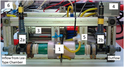
FIGURE 2. Front view of the SGD-MRT: 1. Flow-through unit (FTU), 2 a, b. Conductivity probe at the inflow and outflow of the FTU, 3. Circulation pump to stir fluids inside the FTU, 4. Tracer injection unit (TIU), 5. Three-way tube connector for injection of the saline solution into the FTU, 6. Flexible bag (300 ml) filled with saline water applied for the tracer injection into the FTU. The carrier frame size is L 45 × W 45 × H 18 cm with a weight of about 8 kg.

The main components of the SGD-MRT are the flow-through unit (FTU), conductivity probes (CP), a circulation pump, tracer injection unit (TIU), Arduino controller board, battery pack, and a flexible water bag holding a volume of about 300 ml saline water applied for the tracer injection. A Lee-type chamber collects the fluid discharge from the seabed and connects to the inlet of the FTU via a flexible hose.

One of the central components of the SGD-MRT meter is the FTU (Figures 2, 3), which comprises elastic PVC tubing (ID 50 mm, length 110 mm) and endcaps made from a standard size Delrin rod, which forms the inlet and outlet of the FTU. We installed three-way tube connectors inside each end cap to mound the conductivity probes. The end caps fit into the PVC tubing and can be fixed by pipe clamps. For mixing the fluid inside the FTU, holes (ID 6 mm) were drilled into the PVC pipe and connected by hose to a circulation pump (Figure 3). By shifting the Delrin end caps inside or outside, the inner volume of the FTU for measurements of lower and higher fluid discharge rates can be adjusted.

FIGURE 3

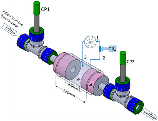
FIGURE 3. Flow-through unit equipped with conductivity probes CP1 and CP2 at the inflow and outflow of the FTU. The water volume inside the FTU is continuously mixed by the circulation pump (1). The TIU (2) injects the saline tracer into the mixing unit (3) to determine the MRT and quantify the fluid discharge rate. The measuring range of the SGD-MRT is adjustable by sliding the Delrin end caps (A) inwards or outwards of the elastic PVC tube (B).

To quantify the conductivity within the inflow and the outflow of the FTU, conductivity probes are used. We decided on a cell constant of K 1.0 and an electronic unit (Atlas Scientific), combining the conductivity probe with the Arduino controller board. The list of components is part of the Supplementary Material.

The TIU – triggered by the Arduino controller – injects a small volume (6 ml) of the sodium chloride solution stored in an elastic storage bag into the FTU (Figure 4). For injection of the tracer, an inexpensive positive displacement gear pump applies (e.g., ModelCraft™). The volumetric flow rate of the gear pump was calibrated in the lab using a laboratory balance and weighing of the water volume pumped for time intervals of 5, 10, or 20 s. For additional quality control, an impeller flow sensor is installed inside the TIU to quantify the saline tracer volume injected into the FTU. We used this procedure as an additional quality control, as the amount of tracer injected is determined during the calculation of the mean residence time.

FIGURE 4

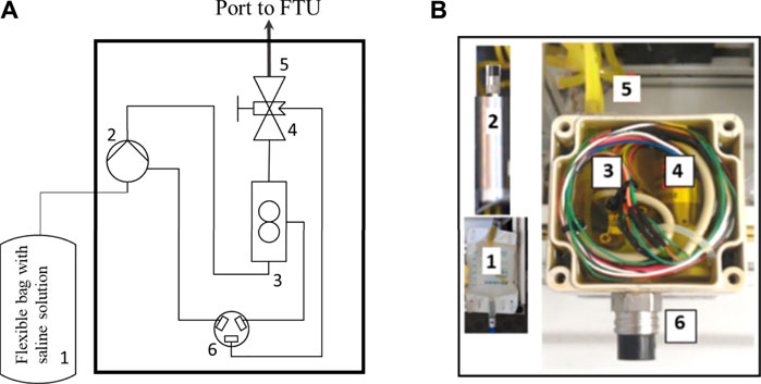
FIGURE 4. Diagram (A) and image (B) of the tracer injection unit (TIU, L 10 × W 10 × H 6 cm). The components of the TIU are 1. a flexible bag filled with the saline solution, 2. gear pump, 3. flow sensor, 4. pinch valve, 5. tracer injection port to the FTU, and 6. cable connector to the Arduino controller.

The components of the TIU reside inside an electric junction box (L 10 × W 10 × H 6 cm), used in households for outdoor electricity cables, for example (Figure 4). We applied such housings for deployments down to 10 m water depths.

Figure 5 shows the schematic wiring diagram and electronic components of the SGD-MRT. The Arduino mega board applies for process control of the SGD-MRT, data acquisition, or data storage. Additional sensors or actuators can extend the controller board. Specific information about the deployment schedule – i.e., the start and end time, the delay time between measurement cycles, and acquired data – are stored on the SD card part of the Arduino controller board.

FIGURE 5

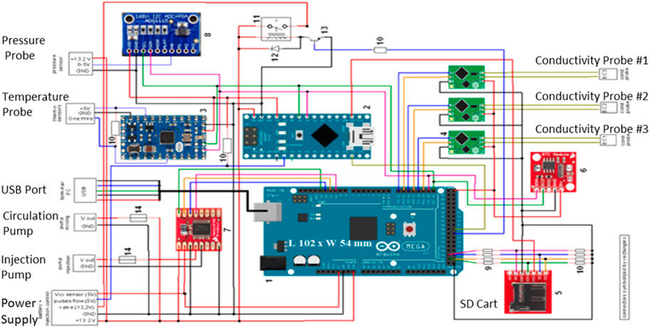
FIGURE 5. Wiring diagram and electronic components of the SGD-MRT. The list of electronic components and the Arduino shields is part of the Supplementary Material.

Process Flow

Beginning with the deployment of the SGD-MRT at the discharge site, the data acquisition starts according to the schedule stored on the Arduino controller board. During the deployment, the conductivity of the fluid at the inlet and outlet of the FTU, the conductivity of the seawater, the hydraulic pressure, or the temperature in the benthic chamber are measured and stored on the SD card. Furthermore, three self-recording Schlumberger CTD divers and temperature probes are installed inside and outside the Lee-type chamber for data acquisition and additional quality control.

In addition to sensors and electronic circuits required to quantify discharge rates, components such as differential pressure gauges (range from 0 to 5 m), temperature sensors, or conductivity probes connect to the Arduino controller board of the SGD-MRT (Figure 5). For example, a conductivity probe is mounted at the bottom of the carrier frame to detect the beginning and end of the inundation of the mudflat.

Triggered by the Arduino controller, a measurement cycle begins with the injection of the saline solution (6 cm³) into the FTU, continuously mixed by a centrifugal pump (Figure 6). The TIU is used for this purpose. The conductivity at the inlet and outlet of the FTU, the time stamp, and additional data are measured every second and stored on the SD card.

FIGURE 6

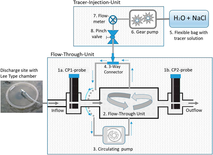
FIGURE 6. Schematic diagram of the process flow: 1a, b. Conductivity probe at inflow (CP1) and outflow (CP2) of the FTU, 2. Flow-through unit (FTU), 3. Circulating pump, 4. Three-way tube connector for tracer injection by the TIU, 5. Flexible bag holding the tracer solution, 6. Gear pump, 7. Impeller flowmeter, and 8. Pinch valve.

Results

Laboratory Tests

The suitability of the SGD-MRT for quantifying the volumetric flow of submarine groundwater discharge was tested first in the laboratory. For this purpose, we applied a simplified constant head tank (Graebel, 2001) to assess the relationship between the volume flow-through the FTU and the computed MRT.

The constant head tank is built from a water drain pipe (L 150 cm, OD 11 cm), available in hardware stores. The pipe is mounted vertically on the laboratory bench and sealed at the lower end of the pipe with an end cap. About 5 cm above the lower end cap of the drainpipe, we installed a pipe connector to couple the drainpipe with the inlet of the FTU and the SGD-MRT by a hose. Above the hose connector, at a vertical distance of 5 cm, we drilled a set of holes (ID 6 mm) with a vertical distance of 5 cm into the drainpipe, which rubber plugs can seal.

To achieve a constant hydraulic pressure and volume flow, we installed the drainpipe vertically on the laboratory bench, closed the boreholes with rubber stoppers up to the desired water level, and filled the pipe continuously from above with water from the tap. The water volume flowing into the drainpipe is slightly higher than the water volume leaving the drainpipe at the bottom. The excess water flows out of the open borehole located above those closed by rubber plugs into the laboratory sink. In this way, we created constant volume flows unaffected by pressure fluctuations caused by other faucets in the laboratory. Furthermore, this procedure mimics the free flow mode of fluid discharge.

For quality control of measurements, the lower outlet of the drain pipe connects to the inlet of the FTU by a hose, and the volume flow leaving the FTU is quantified by the SGD-MRT and by application of a volumetric flask and stopwatch. Through this practice, the volume flow of water is measured simultaneously by two independent methods.

Figure 7 shows an example of the relation between the volumetric flow (υ [cm³/s]) measured by the volumetric cylinder and by the MRT (tm [s]) computed by the SGD-MRT. For example, volume flows of about 80 cm³/min to 780 cm³/min are created by the drainpipe and related to the MRTs of the injected tracer of about 18–90 s (Figure 7). The correlation coefficient and the repeatability of the measurement – indicated by error bars – confirm the suitability of the SGD-MRT to quantify fluid discharge from sediments. We applied these tests as independent validation for the MRT suitability for quantification of volume flows. It should be mentioned that regression analysis is not obligatory for calculating volume flows by the SGD-MRT.

FIGURE 7

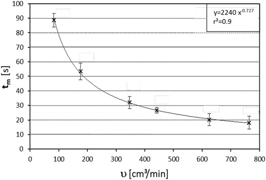
FIGURE 7. Relationship between the volume flow (υ [cm³/min]) and the mean residence time (tm [s]) quantified by the SGD-MRT. The comparison is considered an independent validation of the mean residence time suitability to quantify volume flows.

On-Site Measurements of Fluid Discharge

For the on-site assessment of the SGD-MRT, we deployed the device on the Sahlenburg mudflat on the Elbe-Weser estuary in the southeastern North Sea (Figure 1). This study region is characterized by SGD, extending over an area of at least 1.3 × 4.2 km. Discharge rates of more than 400 cm³/min were measured by Lee-type chambers equipped with flexible sampling bags or impeller flowmeters (Kurtz, 2004; Scharf, 2008; Bartsch, 2009).

For on-site measurements, we selected a discharge site located at the GPS position 53°51′10 ''/8°34′56, and flagged it with a pole for later revisiting this site. At this site, the SGD-MRT was deployed on March 23, 2016 (Sahl#1), for about 6:40 h and June 4, 2016 (Sahl#2), for about 8:20 h. During the deployments, the fluid discharge rates were recorded based on a sampling rate of 6 min.

At the beginning of the time series measurement Sahl#l (Figure 8), the seepage meter measured discharge rates of about 460–500 cm³/min for a period of 96 min during low tide (9:18–10:54). In the following period (10:54–11:24), before inundation reaches the sampling site, a considerable increase of volume flow from about 500 cm³/min to 690 cm³/min within 35 min is observed.

FIGURE 8

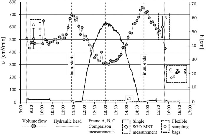
FIGURE 8. Time series data at Sahl#1 of fluid discharge rates (cm³/min) and hydraulic head (cm) measured by the SGD-MRT and the salinity inside the benthic chamber (c1, 2.3 mS/cm) recorded by a CDT diver. The data frames A and B compare discharge rates measured by the SGD-MRT and the flexible sampling bags. Frame C compares discharge rates located aside from the main location. Conventional Lee-type seepage meter measurements are indicated by a grey circle with an error bar. The period of the inundation of the discharge site is indicated by inun.starts and inun.ends.

During the inundation (11:24–13:06), detected by the conductivity probe mounted at the bottom of the carrier frame, discharge rates decrease from about 690 cm³/min to 310 cm³/min within 95 min. With the beginning of the ebb tide (13:06–14:48), a considerable increase in discharge rates from 310 cm³/min to more than 760 cm³/min in about 100 min is recorded. Subsequently, with the end of the inundation (14:48–15:54), discharge rates lowered to about 420 cm³/min, a value comparable to the discharge rate measured at the beginning of the time series measurement (Figure 8).

For comparison purposes, we measured discharge rates at Sahl#1 at the beginning and end of the time series applying the SGD-MRT and flexible sampling bags (Figure 8, frame A and B). This reveals the close comparability of measured volume flows. Additionally, we relocated the Lee-type chamber to a different discharge site in the vicinity, about 5 m aside, of position Sahl#1 to measure discharge rates by the SGD-MRT and flexible sampling bags (Figure 8, frame C). The error bars in frames A, B, and C shows the spread of discharge rates measured by flexible sampling bags. This spread is partially caused by the manual unmounting of the SGD-MRT and mounting of flexible bags. Besides pressure fluctuations, the manual handling close to the discharge sites could cause short-term fluctuations of fluid release, which might cause scatter.

We revisited the discharge site for an additional time series study (Figure 9) on June 4, 2016 (Sahl#2). At low tide, at the beginning of the measurement (9:30–10:36), the SGD-MRT recorded flow rates of about 350 cm³/min. Subsequently, during the transition from low tide to flood tide and inundation of the SGD-MRT, a significant increase of fluid discharges from about 350 cm³/min to 660 cm³/min was observed (10:36–11:12). During the flood tide (11:12–13:42), the water level rose from about 10 to 74 cm, and discharge rates decreased from about 610 cm³/min to less than 70 cm³/min. With the beginning ebb tide, the discharge rate increased to more than 700 cm³/min within 70 min (13:42–15:54). At the end of the inundation, the fluid discharge lowered and reached a value of approximately 400 cm³/min (15:54–17:12). In the following period (17:12–18:00), discharge rates were close to those recorded at the beginning of the deployment.

FIGURE 9

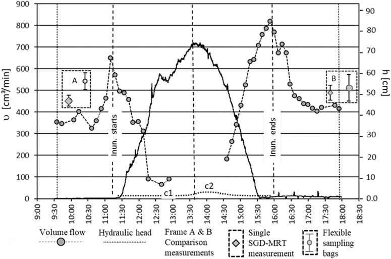
FIGURE 9. Time series data (Sahl#2) of fluid discharge rates (cm³/min), and the hydraulic head (cm) measured by the SGD-MRT and the salinity inside the benthic chamber (c1: 2.9 mS/cm, c2: 5.2 mS/cm) recorded by a CDT diver. In data frames A and B, discharge rates measured with the SGD-MRT and flexible sampling bags compare conventional Lee-type seepage meter measurements indicated by a grey circle with an error bar. The period of the inundation of the discharge site is marked by inun.starts and inun.ends.

For comparison purposes, the outflow rates were quantified with the SGD-MRT and flexible sampling bags at the beginning and at the end of the time series measurement (Figures 8, 9). Due to the uncoupling and coupling of the flexible bags to the Lee-Type chamber, counter pressures influence the discharge of fluid from the sand boil. Despite these effects, the measurements with flexible bags are close to the discharge rates that were quantified by the time-series measurements of the SGD-MRT.

During the period of 15:45–16:15, the tidal height at the discharge site rose to 74 cm, and the salinity measured by the CTD diver mounted in the benthic chamber increased from approximately 2.9 mS/cm to 5.2 mS/cm and back to 2.9 mS as at the beginning of the ebb (Figure 9). The slight increase in salinity in the Lee-Type chamber indicates a small volume of bottom water entering the benthic chamber along with the FTU.

Discussion

The main driving forces for the release of groundwater from sediments are hydraulic pressure gradients between the landward aquifer and the intertidal zone or pressure fluctuations caused by tidal cycles. The pressure-driven transport of fluids occurs as a dispersed flow through the pore space of unconsolidated sediment or as conduit flow along pipe-like transport pathways. The latter could cause the formation of boils, discharge sites with intensive release of fluids, or sand boils (Figure 1B), areas with an intensive discharge of fluids and washing out of fine-grained particles into bottom waters (Kolb, 1976; Bardet and Kapuskar, 1991; Holzer and Clark, 1993; Li et al., 1996; de Louw et al., 2010; Sassa and Takagawa, 2018). Despite the number of sand boils observed on land or in shallow waters of coastal regions, lakes, or rivers, it appears that discharge rates are rarely quantified to the best of our knowledge.

Sand boils (Figure 1B), sites with an intensive fluid discharge are observed in coastal waters, lakes, dams, or polders (de Louw et al., 2010). For example, for landward saline sand boils on a Polder region in the Netherlands, discharge rates of 500–1,000 dm³/day were quantified by hydrogeological techniques (de Louw et al., 2010; Pauw et al., 2012). In contrast to the onshore sand boils, almost fresh water released from sand boils on the Sahlenburg Mudflat with discharge rates of more.

To account for the broad range of fluid discharges with volume flows of less than 5 cm³/min to more than 20 cm³/min and different transport modes like the dispersed or the conduit transport of fluids, numerous techniques have been developed. For the quantification of fluid releases of less than 5 cm³/min, for example, techniques such as pore water analysis of chloride profiles and calculation of advection rates or methods such as heat pulse injection or dye displacement methods are in use (Vanek, 1993; Schlüter et al., 2004; Seeberg-Elverfeldt et al., 2005; Taniguchi et al., 2007; Koopmans and Berg, 2011; Taniguchi et al., 2019). Quantifying discharge rates of more than 20 cm³/min, mainly seepage meters are used, comprising a Lee-type chamber and a flexible sampling bag or an automated, self-recording flow sensor. This includes impeller-based flow meters or techniques such as the heat pulse injection, or dye dilution method.

Both the automated dye-dilution based seepage meter and the SGD-MRT apply a tracer injection method, suitable for quantification of discharge rates of more than 60 cm³/min. For the dye dilution method, an exponential curve fitting routine is required to determine the flow rates based on the absorption measurements recorded by the underwater photometer. Furthermore, concentration of the dye solution needs to be adjusted according to the volume of the dye-mixing chamber to provide a strong initial absorbance signal for the dyed solution without exceeding the linear response (Beer’s Law) range of the photometer.

In contrast to most other tracer injection methods, we apply the computation of the Mean Residence Time for quantifying flow rates. A specific flow sensor is not required for this purpose, instead, the concentration-time distribution of the electric conductivity measured at the outflow of the FTU is recorded and analyzed. By this means, the total amount of tracer injected is quantified by numerical integration. This allows analyzing the concentration-time distribution over the entire sampling period in order to quantify the mean residence time and volume flow of fluids.

For the data derived from deployments Sahl#1 and Sahl#2, we calculated the total amount of water released from the discharge by numerical integration of the measured flow rates. Considering the time-series record of Sahl#1, about 400 dm³ of water was released from the discharge site within 6:30 h. At Sahl#2 a water volume of about 360 dm³ was released over a period of 8:30 h. On a daily basis, this suggests an SGD volume of more than 700 dm³/day released from a discharge site. For groundwater management in coastal regions, boils and sand boils seem to be efficient transport routes between land and sea, which can change the direction of flow depending on the hydraulic pressure conditions.

Process Control and Data Acquisition

Applying the MRT, a designated flow sensor is not required for quantifying discharge rates. Instead, the combination of FTU, tracer injection, conductivity probes, Arduino controller, and the software builds the measuring unit. In addition to these components, differential pressure sensors, temperature probes, or conductivity probes are installed inside the benthic chamber or on the carrier frame and connected to the controller unit (Figure 5). These components are used for additional quality control or to extend the scope of the SGD-MRT. Due to this design, the measuring range, the sampling rate, or other settings could be adjusted.

The Arduino controller runs the source code – which is part of the Supplementary Material – and manages the process control, data acquisition, or data storage. The sampling rate and other settings could be modified by editing the ini-file stored on the SD card. Furthermore, actuators like an injection pump, differential pressure sensors, temperature probes, or conductivity probes are installed inside the benthic chamber or on the carrier frame and connected to the controller board. By this means, the tidal height, conductivity of fluids, or temperature inside the Lee-type chamber, bottom water, or sediment are recorded. For the time series recording of the tracer concentration at the outflow of the FTU and calculation of the discharge rates, the conductivity in the inlet and outlet of the FTU is measured every second.

Due to the modular concept and the comparatively inexpensive electronic components, Arduino microcontrollers are applied in numerous applications and fields spanning the arts to science or industry. In contrast to terrestrial environmental studies, Arduino or similar microcontrollers seem to have only been used for a few studies on marine or limnology research. An example is the development-inexpensive Arduino-based CDT probe for studies in coastal waters (Lockridge, 2016). Due to the large community of users applying Arduino boards, the modular concept, and the comparatively inexpensive electronic components, these microcontrollers can be easily expanded with SD memory cards, motor controllers, peristaltic pumps for water sampling, or sensors for numerous applications.

The estimated system costs for the SGD-MRT – excluding the CDT diver, pressure housings, and underwater cables – might be about 1,500 €. A re-design concerning the number of pressure housings or cables is feasible (Figure 5).

Seawater Fresh Water Ratio

On sampling date Sahl#1, applying a CDT diver, a conductivity of about 2.1 mS/cm was recorded for fluids inside the benthic chamber, and a conductivity of 28.5 mS/cm was recorded for the bottom water aside from the benthic chamber. According to the conductivity ratio calculated, the released fluids comprise more than 93% fresh water.

During the field trials on Sahl#2, the CDT diver mounted at the bottom of the carrier frame recorded a conductivity of 27 mS/cm. Inside the benthic chamber, a conductivity of 2.5 mS/cm was measured for the periods from 9:30 to 12:50 and from 14:30 to 18:00 (Figure 9). In the time interval from 12:50 to 14:30, when the hydraulic head exceeded 74 cm, conductivity inside the benthic chamber increased from 2.5 mS/cm to 5.2 mS/cm, indicating a low input of seawater into the benthic chamber. Based on the internal volume of the benthic chamber of around 9 dm³, a seawater conductivity of 27 mS/cm, and the increase in conductivity inside the benthic chamber from 2.5 to 5.0 mS/cm, the estimated input of seawater into the benthic chamber results in approximately 1.2 dm³.

The time series data of fluid discharge was interrupted at Sahl#2 on 12:50 at a discharge rate of 97 cm³/min and continued from 14:40 at a flow rate of about 195 cm³/min. During this period, the conductivity inside the benthic chamber – measured by the CTD diver – increased from 2.7 mS/cm to 5.1 mS/cm at 14:00 and levels back to the initial conductivity at 14:40 (Figure 9). In the following, the measurement of discharge rates steadily continued. As indicated by the slight increase of conductivity of 2.4 mS/cm, related to the bottom water conductivity of 25 mS/cm, only a small volume of seawater might intrude into the benthic chamber.

For more detailed considerations about the data gap, the conductivities measured every second at the inlet and outlet of the FTU were investigated. During the time interval of the data gap, the fluid conductivity inside the FTU varies in a bell-shape mode, from 2.7 mS/cm at 12:50 to 12.2 mS/cm at 13:45 and back to 2.7 mS/cm at 14:45. The increase of conductivity is caused by the TIU, injecting the saline tracer into the FTU every 6 min. Due to the nearly stagnant flow conditions inside the FTU, the conductivity increases and masks the saline tracer and conductivity inside the FTU. With the restart of the fluid discharge from the discharge site, the FTU flushed, and the measurement of discharge rates continue. By modifying the Arduino source code, for example, by adding a feedback loop, this situation can be avoided.

Fluid Discharge From Sand Boils

Sand boils are observed offshore and landward in rivers, lakes, water reservoirs, harbor areas, or low-lying coastal regions. For example, at landward, at polders along the Dutch coastline, numerous sand boils with intense fluid discharge are observed (de Louw et al., 2010). In this region, saline waters with an average chloride concentration of 1,100 mg/L are released from the landward sand boil, and discharge rates of 500–1,000 dm³/day are reported.

For the Sahlenburg mudflat, we computed the total volume of water released from the discharge site by numerical integration of the measured flow rates. At the date Sahl#1, a water volume of 400 dm³ was released from the discharge site within 6:30 h, and during a period of 8:30 h a water volume of 360 dm³ was released from Sahl#2. On a daily basis, this suggests a SGD of more than 700 dm³/day. Regarding groundwater management in coastal regions, sand boils seem to be efficient transport routes between land and sea, which can change the direction of flow according to the hydraulic pressure conditions.

Conclusion

The motivation for developing SGD-MRT was our demand for an inexpensive and extensible seepage meter suitable for recording time series data of fluid discharge from sand boils. Previous attempts to quantify discharge rates of more than 200 cm³ were only partially successful. Systems like the scalable SGD-MRT, with a measuring range of up to 700 cm³/min, might support such objectives.

The modular structure of the SGD-MRT and the use of microcontrollers such as the Arduino offers numerous possibilities for additional applications. In particular, the studies on fluid transport along sand boils connecting the land and coastal waters could support local studies on groundwater management in coastal areas.

Data Availability Statement

The raw data supporting the conclusion of this article will be made available by the authors, without undue reservation.

Author Contributions

MS developed the tracer inject method concept and built the first versions of the seepage meter, including the electronics and Arduino software. PM compiled the final version of the SGD-MRT, improved and updated the existing software, and operated the field trials.

Conflict of Interest

The authors declare that the research was conducted in the absence of any commercial or financial relationships that could be construed as a potential conflict of interest.

Publisher’s Note

All claims expressed in this article are solely those of the authors and do not necessarily represent those of their affiliated organizations, or those of the publisher, the editors and the reviewers. Any product that may be evaluated in this article, or claim that may be made by its manufacturer, is not guaranteed or endorsed by the publisher.

Acknowledgments

We acknowledge the support by the “Wadden Sea World Heritage Center” (Sahlenburg, Germany; https://www.waddensea-worldheritage.org/), the two reviewers, and Henry Bokuniewicz (Stony Brook University) for their very constructive advice.

Supplementary Material

The Supplementary Material for this article can be found online at: https://www.frontiersin.org/articles/10.3389/feart.2021.710000/full#supplementary-material

References

Bardet, J. P., and Kapuskar, M. (1991). The Liquefaction Sand Boils in the San Francisco Marina District during the 1989 Loma Prieta Earthquake. Los Angeles, California: Second International Conference on Recent Advances in Geotechnical Earthquake Engineering University of Southern California. Available at: https://scholarsmine.mst.edu/cgi/viewcontent.cgi?article=3629&context=icrageesd.

Bartsch, S. (2009). Erfassung von Porenwasservariationen in Wattsedimenten und der Einfluss von Grundwasseraustritt im Sahlenburger Watt. Bremen: Geoscience, FB5, 178.

Bokuniewicz, H. (1980). Groundwater Seepage into Great South Bay, New York. Estuar. Coast. Mar. Sci. 10, 437–444. doi:10.1016/S0302-3524(80)80122-8

CrossRef Full Text | Google Scholar

Bugna, G. C., Chanton, J. P., Cable, J. E., Burnett, W. C., and Cable, P. H. (1996). The Importance of Groundwater Discharge to the Methane Budgets of Nearshore and continental Shelf Waters of the Northeastern Gulf of Mexico. Geochim. Cosmochim. Acta 60, 4735–4746. doi:10.1016/s0016-7037(96)00290-6

CrossRef Full Text | Google Scholar

Burnett, W. C., Aggarwal, P. K., Aureli, A., Bokuniewicz, H., Cable, J. E., Charette, M. A., et al. (2006). Quantifying Submarine Groundwater Discharge in the Coastal Zone via Multiple Methods. Sci. Total Environ. 367, 498–543. doi:10.1016/j.scitotenv.2006.05.009

PubMed Abstract | CrossRef Full Text | Google Scholar

Burnett, W. C., Bokuniewicz, H., Huetel, M., Moore, W. S., and Taniguchi, M. (2003). Groundwater and Pore Water Inputs to the Coastal Zone. Biogeochemistry 66, 3–33. doi:10.1023/B:BIOG.0000006066.21240.53

CrossRef Full Text | Google Scholar

Cable, J. E., Martin, J. B., and Jaeger, J. (2006). Exonerating Bernoulli? on Evaluating the Physical and Biological Processes Affecting marine Seepage Meter Measurements. Limnol Ocean Methods 172–183, 4–6. doi:10.4319/lom.2006.4.172

PubMed Abstract | CrossRef Full Text | Google Scholar

Cherkauer, D. A., and McBride, J. M. (1988). A Remotely Operated Seepage Meter for Use in Large Lakes and Rivers. Westerville, Ohio, USA: Ground Water, 165–171. doi:10.1111/j.1745-6584.1988.tb00379.x

CrossRef Full Text

Clark, M. M. (1996). Transport Modelling for Environmental Engineers and Scientists. Wiley-Interscience, 559.

Danckwerts, P. V. (1953). Continuous Flow Systems: Distribution of Residence Times. Chem. Eng. Sci. 2, 1–13. doi:10.1016/0009-2509(53)80001-1

CrossRef Full Text | Google Scholar

de Louw, P. G. B., Essink, O. G. H. P., Stuyfzand, P. J., and van der Zee, S. E. A. T. M. (2010). Upward Groundwater Flow in Boils as the Dominant Mechanism of Salinization in Deep Polders, The Netherlands. J. Hydrol. 394, 494–506. doi:10.1016/j.jhydrol.2010.10.009

CrossRef Full Text | Google Scholar

Duque, C., Russoniello, C. J., and Rosenberry, D. O. (2020). History and Evolution of Seepage Meters for Quantifying Flow between Groundwater and Surface Water: Part 2 – Marine Settings and Submarine Groundwater Discharge. Earth-Science Rev. 204, 1. doi:10.1016/j.earscirev.2020.103168

CrossRef Full Text | Google Scholar

Fogler, S. (2006). Elements of Chemical Reaction Engineering. 3. ed. Hoboken, New Jersey, USA: Prentice-Hall.

Graebel, W. P. (2001). Engineering Fluid Mechanics. Taylor & Francis, 675.

Holzer, T. L., and Clark, M. M. (1993). Sand Boils without Earthquakes. Geology 21 (10), 873–876. doi:10.1130/0091-7613(1993)021<0873:sbwe>2.3.co;2

CrossRef Full Text | Google Scholar

Johannes, R. E. (1980). The Ecological Significance of Submarine Discharge of Groundwater. Mar. Ecol. 3, 365–373. doi:10.3354/meps003365

CrossRef Full Text | Google Scholar

Judd, A., and Hovland, M. (2009). Seabed Fluid Flow. Cambridge University Press. doi:10.1017/CBO9780511535918

CrossRef Full Text

Kolb, C. R. (1976). “Geologic Control of Sand Boils along Mississippi River Levees,” in Geomorphology and Engineering: Stroudsburg. Editor D. R. Coates (Pennsylvania: Halstead Press), 99–114. Available at: https://erdc-library.erdc.dren.mil/jspui/bitstream/11681/20960/1/MP-S-75-22.pdf.

Google Scholar

Koopmans, D., and Berg, P. (2011). An Alternative to Traditional Seepage Meters: Dye Displacement. Water Resour. Res. 47, W01506. doi:10.1029/2010WR009113

CrossRef Full Text | Google Scholar

Kurtz, S. (2004). Grundwasseraustrittsstellen im Sahlenburger Watt: Methoden zur Beprobung von Fluiden und Bilanzierung des Grundwasserausstroms. Bremen: Univ. Bremen, FB5.

Lee, D. R. (1977). A Device for Measuring Seepage Flux in Lakes and Estuaries. Limnol.Oceanogr. 22, 140–147. doi:10.4319/lo.1977.22.1.0140

CrossRef Full Text | Google Scholar

Levenspiel, O. (1999). Chemical Reaction Engineering. Wiley, 668p. 0-471-25424-X.

Li, Y., Craven, J., Schweig, E. S., and Obermeier, S. F. (1996). Sand Boils Induced by the 1993 Mississippi River Flood: Could They One Day Be Misinterpreted as Earthquake-Induced Liquefaction? Geology 24, 171–174. doi:10.1130/0091-7613(1996)024<0171:sbibtm>2.3.co;2

CrossRef Full Text | Google Scholar

Lockridge (2016). Development of a Low-Cost Arduino-Based Sonde for Coastal Applications. Sensors 16, 528. doi:10.3390/s16040528

PubMed Abstract | CrossRef Full Text | Google Scholar

Martin, J. B., Thomas, R. G., and Hartl, M. K. (2004). An Inexpensive, Automatic, Submersible Water Sampler. Limnol. Oceanogr. Methods 2, 398–405. doi:10.4319/lom.2004.2.398

CrossRef Full Text | Google Scholar

Moore, W. S. (1996). Large Groundwater Inputs to Coastal Waters Revealed by 226Ra Enrichments. Nature 380, 612–614. doi:10.1038/380612a0

CrossRef Full Text | Google Scholar

Moore, W. S. (1999). The Subterranean Estuary: a Reaction Zone of Ground Water and Seawater. Mar. Chem. 65, 111–125. doi:10.1016/S0304-4203(99)00014-6

CrossRef Full Text | Google Scholar

Murdoch, L. C., and Kelly, S. E. (2003). Factors Affecting the Performance of Conventional Seepage Meters. Water Resour. Res. 39, 1. doi:10.1029/2002WR001347

CrossRef Full Text | Google Scholar

Pauw, P., de Louw, P. G. B., and Oude Essink, G. H. P. (2012). Groundwater Salinisation in the Wadden Sea Area of the Netherlands: Quantifying the Effects of Climate Change, Sea-Level Rise and Anthropogenic Interferences. Neth. J. Geosciences 91, 373–383. doi:10.1017/s0016774600000500

CrossRef Full Text | Google Scholar

Povinec, P. P., Burnett, W. C., Beck, A., Bokuniewiczc, H., Charette, M., Gonneead, M. E., et al. (2012). Isotopic, Geophysical and Biogeochemical Investigation of Submarine Groundwater Discharge: IAEA-UNESCO Intercomparison Exercise at Mauritius Island. J. Environ. Radioactivity 104, 24–45. doi:10.1016/j.jenvrad.2011.09.009

PubMed Abstract | CrossRef Full Text | Google Scholar

Rocha, C., Ibanhez, J. B., and Leote, C. (2009). Benthic Nitrate Biogeochemistry Affected by Tidal Modulation of Submarine Groundwater Discharge (SGD) through a sandy beach Face, Ria Formosa, Southwestern Iberia. Mar. Chem. 115, 43–58. doi:10.1016/j.marchem.2009.06.003

CrossRef Full Text | Google Scholar

Rosenberry, D. O. (2008). A Seepage Meter Designed for Use in Flowing Water. J. Hydrol. 359 (1–2), 118–130. doi:10.1016/j.jhydrol.2008.06.029

CrossRef Full Text | Google Scholar

Rosenberry, D. O., Duque, C., and Lee, D. R. (2020). History and Evolution of Seepage Meters for Quantifying Flow between Groundwater and Surface Water: Part 1 – Freshwater Settings. Earth-Science Rev. 204, 1. doi:10.1016/j.earscirev.2020.103167

CrossRef Full Text | Google Scholar

Santos, I. R., Burnett, W. C., Chanton, J., Dimova, N., and Peterson, R. N. (2009). Land or Ocean?: Assessing the Driving Forces of Submarine Groundwater Discharge at a Coastal Site in the Gulf of Mexico. J. Geophys. Res. 114, 2156–2202. doi:10.1029/2008JC005038

CrossRef Full Text | Google Scholar

Sassa, S., and Takagawa, T. (2018). “Liquefied Gravity Flow-Induced Tsunami: First Evidence and Comparison from the 2018 Lndonesia Sulawesi Earthquake and Tsunami Disasters,” in News/Kyoto Commitment. Ministry of Land, Infrastructure, Transport and Tourism (MLIT) (Japan: MLIT). doi:10.1007/s10346-018-1114-x

CrossRef Full Text | Google Scholar

Scharf, F. (2008). Der Grundwasseraustritt im Sahlenburger Watt bei Cuxhaven: Datenerhebung und GIS-basierte Untersuchung der Ursachen und Charakteristiken. Bremen: Uni. Bremen, Geoscience, FB5, 137 p.

Schlüter, M., SauterAndersen, E. J. C. E., Dahlgaard, H., and Dando, P. R. (2004). Spatial Distribution and Budget for Submarine Groundwater Discharge in Eckernfoerde Bay (Western Baltic Sea). Limnol. Oceanogr. 49 (1), 157–167. doi:10.4319/lo.2004.49.1.0157

CrossRef Full Text | Google Scholar

Seeberg-Elverfeldt, J., Schlüter, M., Feseker, T., and Kölling, M. (2005). Rhizon Sampling of Porewaters Near the Sediment-Water Interface of Aquatic Systems. Limnol. Oceanogr Methods 3, 361–371. doi:10.4319/lom.2005.3.361

CrossRef Full Text | Google Scholar

Shaw, R. D., and Prepas, E. E. (1990). Groundwater‐lake Interactions: I. Accuracy of Seepage Meter Estimates of lake Seepage. J. Hydrol. 119 (1–4), 105–120. doi:10.1016/0022-1694(90)90037-X

CrossRef Full Text | Google Scholar

Sholkovitz, E. R., Herbold, C. W., and Charette, M. A. (2003). An Automated Dye-Dilution Based Seepage Meter for the Time-Series Measurement of Submarine Groundwater Discharge. Limnol. Oceanogr. Methods 1, 16–28. doi:10.4319/lom.2011.1.16

CrossRef Full Text | Google Scholar

Simmons, G. M. (1992). Importance of Submarine Groundwater Discharge (SGWD) and Seawater Cycling to Material Flux across Sediment/water Interfaces in marine Environments. Mar. Ecol. Prog. Ser. 84, 173–184. doi:10.3354/meps084173

CrossRef Full Text | Google Scholar

Solomon, D. K., Humphrey, E., Gilmore, T. E., Genereux, D. P., and Zlotnik, V. (2020). An Automated Seepage Meter for Streams and Lakes. Water Resour. Res. 1, 1–11. doi:10.1029/2019WR026983

CrossRef Full Text | Google Scholar

Taniguchi, M., Dulai, H., Burnett, K. M., Santos, I. R., Sugimoto, R., Stieglitz, T., et al. (2019). Submarine Groundwater Discharge: Updates on its Measurement Techniques, Geophysical Drivers, Magnitudes, and Effects. Westerville, Ohio, USA: Frontiers in Environmental Science. doi:10.3389/fenvs.2019.00141

CrossRef Full Text

Taniguchi, M., and Fukuo, Y. (1993). Continuous Measurements of Groundwater Seepage Using an Automatic Seepage Meter. Groundwater 31, 675–679. doi:10.1111/j.1745-6584.1993.tb00601.x

CrossRef Full Text | Google Scholar

Taniguchi, M., Ishitobi, T., Burnett, W. C., and Wattayakorn, G. (2007). Evaluating Ground Water-Sea Water Interactions via Resistivity and Seepage Meters. Ground Water 45 (6), 729–735. doi:10.1111/j.1745-6584.2007.00343.x

PubMed Abstract | CrossRef Full Text | Google Scholar

Vanek, V. (1993). Groundwater Regime of a Tidally Influenced Coastal Pond. J. Hydrol. 151 (2-4), 317–342. doi:10.1016/0022-1694(93)90241-z

CrossRef Full Text | Google Scholar

Zektzer, I. S., Ivanov, V. A., and Meskheteli, A. V. (1973). The Problem of Direct Groundwater Discharge to the Seas. J. Hydrol. 20, 1–36. doi:10.1016/0022-1694(73)90042-5

CrossRef Full Text | Google Scholar

Zimmermann, C. F., Montgomery, J. R., and Carlson, P. R. (1985). Variability of Dissolved Reactive Phosphate Flux Rates in Nearshore Estuarine Sediments: Effects of Groundwater Flow. Estuaries 8, 228–236. doi:10.2307/1352203

CrossRef Full Text | Google Scholar