
94% of researchers rate our articles as excellent or good
Learn more about the work of our research integrity team to safeguard the quality of each article we publish.
Find out more
ORIGINAL RESEARCH article
Front. Earth Sci., 24 November 2021
Sec. Interdisciplinary Climate Studies
Volume 9 - 2021 | https://doi.org/10.3389/feart.2021.702285
This article is part of the Research TopicPast Reconstruction of the Physical and Biogeochemical Ocean StateView all 13 articles
 Romain Escudier1*†
 Emanuela Clementi1
 Andrea Cipollone1
 Jenny Pistoia1
 Massimiliano Drudi2
 Alessandro Grandi2
 Vladislav Lyubartsev2
 Rita Lecci2
 Ali Aydogdu1
 Damiano Delrosso3
 Mohamed Omar1‡
 Simona Masina1
 Giovanni Coppini1
 Nadia Pinardi4
In order to be able to forecast the weather and estimate future climate changes in the ocean, it is crucial to understand the past and the mechanisms responsible for the ocean variability. This is particularly true in a complex area such as the Mediterranean Sea with diverse dynamics like deep convection and overturning circulation. To this end, effective tools are ocean reanalyses or reconstructions of the past ocean state. Here we present a new physical reanalysis of the Mediterranean Sea at high resolution, developed in the Copernicus Marine Environment Monitoring Service (CMEMS) framework. The hydrodynamic model is based on the Nucleus for European Modelling of the Ocean (NEMO) combined with a variational data assimilation scheme (OceanVar). The model has a horizontal resolution of 1/24° and 141 unevenly distributed vertical z* levels. It provides daily and monthly temperature, salinity, current, sea level and mixed layer depth as well as hourly fields for surface velocities and sea level. ECMWF ERA-5 atmospheric fields force the model and daily boundary conditions in the Atlantic are taken from a global reanalysis. The reanalysis covers the 33 years from 1987 to 2019. Initialized from SeaDataNet climatology in January 1985, it reaches a nominal state after a 2-years spin-up. In-situ data from CTD, ARGO floats and XBT are assimilated into the model in combination with satellite altimetry observations. This reanalysis has been validated and assessed through comparison to in-situ and satellite observations as well as literature climatologies. The results show an overall improvement of the comparison with observations and a better representation of the main dynamics of the region compared to a previous, lower resolution (1/16°), reanalysis. Temperature and salinity RMSD are decreased by respectively 14 and 18%. The salinity biases at depth of the previous version are corrected. Climate signals show continuous increase of the temperature and salinity, confirming estimates from observations and other reanalysis. The new reanalysis will allow the study of physical processes at multi-scales, from the large scale to the transient small mesoscale structures and the selection of climate indicators for the basin.
Reanalysis is a crucial tool to understand the events of the past and help us find the underlying processes that should be represented by the numerical models. Reanalysis products are computed by constraining a numerical model with available observations using data assimilation. They have been used extensively in ocean sciences (Storto et al., 2019) as they provide 4D fields that correspond to the best estimate of the ocean state. Atmospheric models and observations are introduced into the system through the surface forcings, ocean physics through the ocean global circulation model (OGCM) and finally the data assimilation scheme adds the ocean observations.
Ocean reanalyses were initially computed to monitor and understand climate change (e.g., Carton and Santorelli 2008). They also allow to study important signals and processes that cannot be observed completely such as deep water formation (e.g., Somot et al., 2016), subsurface and bottom circulation (Pinardi et al., 2015) or the overturning circulation (Pinardi et al., 2019). In addition, subregional models need the reanalyses as initial conditions and boundary conditions. In the Mediterranean Sea, there are different models that uses the Mediterranean reanalysis for their setup such as the Adriatic Forecasting System (Oddo et al., 2005), the Sicily Channel Regional Model (Olita et al., 2012), the Tyrrhenian Sea Forecasting (Vetrano et al., 2010) or the Western Mediterranean OPerational forecasting system (WMOP, Juza et al., 2016).
The Mediterranean Sea is a challenging area with a strong anthropogenic pressure due to the density of human population living along its coasts (Hulme et al., 1999). It is therefore crucial to study and understand the climate in this region and it has been flagged as a hotspot for climate change (Giorgi, 2006). In this semi-enclosed sea, many fundamental processes that occur in the global ocean happen at a smaller scale, often called a miniature ocean (Bethoux et al., 1999; Tsimplis et al., 2006). Examples of these processes are mesoscale dynamics (Robinson et al., 2001; Mkhinini et al., 2014; Escudier et al., 2016), deep convection (MEDOC Group et al., 1970; Houpert et al., 2016), cascading (Dufau-Julliand et al., 2004) or the overturning circulation in the basin (Pinardi et al., 2019). The increased understanding and upgrade of ocean forecasting products depends on the ability to maintain the observing system and the progressive inclusion of relevant processes in numerical models, especially in view of the climate challenges facing the Mediterranean Sea (Tintoré et al., 2019).
The first effort to compute a reanalysis for the Mediterranean Sea was made by Adani et al. (2011). This reanalysis used the OPA numerical model (Océan PArallélisé, Madec et al., 1997) on a 1/16° regular horizontal grid (Tonani et al., 2008). Evolutions of this reanalysis became a product in Copernicus Marine Environment Monitoring Service (CMEMS), which represents the previous version of the reanalysis presented here (Simoncelli et al., 2016; Simoncelli et al., 2019). It will be hereafter referred as MEDREA16. Another reanalysis (MEDRYS) was created to address mainly the issue of inconsistency in the atmospheric forcing (Hamon et al., 2016). For this product, special attention was given to the atmospheric forcing using consistent and higher resolution data. It showed the importance of the atmospheric forcing to fully resolve the dynamics.
In this paper, we present a new reanalysis of the Mediterranean Sea physical state performed in the framework of CMEMS for the period 1987–2019 (Escudier et al., 2020). CMEMS objective is to provide regular information on the ocean state for the global ocean and European regional seas such as the Mediterranean (Le Traon et al., 2019). In order to fulfill this mission, they offer freely available descriptions of the current ocean state (analysis), predictions of the situation 10 days ahead (forecast), and the provision of consistent retrospective data records (reprocessing and reanalysis). The new reanalysis is part of the latter for the Mediterranean region and is the current available product on the CMEMS website: https://marine.copernicus.eu/. It is a significant upgrade from the previously available product in CMEMS (MEDREA16) and it will address some issues that were encountered such as biases in the deeper layers (Juza et al., 2015). The new reanalysis, computed on a 1/24° horizontal grid, will be hereafter called MEDREA24.
After describing all the elements of the system, we will assess its performance by comparing it to observations, evaluate the climate signals from the reanalyses and finish with a discussion on the results.
The oceanic equations of motion of the Mediterranean physical system are solved by an Ocean General Circulation Model (OGCM) based on NEMO (Nucleus for European Modelling of the Ocean) version 3.6 (Madec et al., 2017). The code is developed and maintained by the NEMO-consortium.
NEMO has been implemented in the Mediterranean at 1/24° x 1/24° horizontal resolution and 141 unevenly spaced vertical levels (thickness is 2 m in the upper layers and does not exceed 100 m in the deepest layers) with a baroclinic time step of 240 s (the barotropic time step is 2.4 s). This reanalysis benefits from several modeling upgrades that were included during the last years in the CMEMS Mediterranean operational analysis and forecast system described in Clementi et al. (2017). The model covers the whole Mediterranean Sea and also extends into the Atlantic in order to better resolve the exchanges with the Atlantic Ocean at the Strait of Gibraltar (see Figure 1). On the other side, the Dardanelles inflow is parameterized as a river and the climatological net inflow rates as well as the salinity values are taken from Kourafalou and Barbopoulos (2003). The topography is created starting from the GEBCO 30arc-second grid (Weatherall et al., 2015), filtered (using a Shapiro filter) and manually modified in critical areas such as: islands along the Eastern Adriatic coasts, Gibraltar and Messina straits, Atlantic box edge.
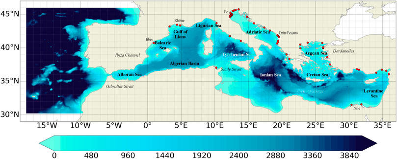
FIGURE 1. Domain and bathymetry of MEDREA24 (in meters). Position of the river input are in red.
The NEMO code solves the primitive equations using the time-splitting technique which allows the external gravity waves to be explicitly resolved with non-linear free surface formulation and time-varying vertical z* coordinates. The advection scheme for active tracers, temperature and salinity, is a mixed up-stream/MUSCL (Mono-tonic Upwind Scheme for Conservation Laws; Van Leer 1979), originally implemented by Estubier and Lévy (2000) and modified by Oddo et al. (2009). The vertical diffusion and viscosity terms are a function of the Richardson number as parameterized by Pacanowski and Philander (1981). The model interactively computes air-surface fluxes of momentum, mass, and heat. The bulk formulae implemented are described in Pettenuzzo et al. (2010) and are currently used in the Mediterranean operational system Tonani et al. (2015). A detailed description of other specific features of the model implementation can be found in Oddo et al. (2009, 2014).
The vertical background viscosity and diffusivity values are set to 1.2e−6 m2/s and 1.0e−7 m2/s respectively, while the horizontal bilaplacian eddy diffusivity and viscosity are set respectively equal to −1.2e8m4/s and − 2e8m4/s. A quadratic bottom drag coefficient with a logarithmic formulation has been used according to Maraldi et al. (2013) and the model uses vertical partial cells to fit the bottom depth shape.
The hydrodynamic model is nested in the Atlantic within the global reanalysis C-GLORSv5 (Storto and Masina, 2016). C-GLORSv5 runs at eddy-permitting resolution (1/4° horizontal resolution and 50 vertical levels) and is corrected by a variational data assimilation system (OceanVar) that assimilates in-situ observation from United Kingdom Met Office Hadley Centre EN3/EN4 dataset (Good et al., 2013) together with along-track altimetric satellite observations processed by the DUACS multimission altimeter data processing system and also available as CMEMS product (SEALEVEL_GLO_PHY_L3_REP_OBSERVATIONS_008_062). Heat and freshwater fluxes are constrained through nudging schemes towards sea-surface temperature observations supplied by NOAA (Reynolds et al., 2007) and sea surface salinity from OI EN4 dataset (Good et al., 2013). A large-scale bias correction (LSBC) scheme is also included to correct the model tendencies.
The initial conditions for MEDREA24 are taken from a temperature and salinity monthly climatology computed from monthly averages (named SDN_V2aa, Simoncelli et al., 2015) produced within It has been calculated utilizing the extensive historical in situ data set from 1900 to 1987. We considered only observations before 1987 to compute the initial condition because we did not want the climatology to be affected by the Eastern Mediterranean Transient (EMT, see Malanotte-Rizzoli et al., 1999).
The model is forced by momentum, water and heat fluxes interactively computed by bulk formulae using the ERA5 reanalysis dataset (30 km horizontal resolution and hourly time frequency, Hersbach et al., 2020) and the model surface temperatures (details of the air-sea physics are in Tonani et al., 2008). The water balance is computed as Evaporation minus Precipitation and Runoff. The evaporation is derived from the latent heat flux, the precipitations are provided by ERA5, while the runoff of the 39 rivers implemented is provided by monthly mean climatological datasets. We use the Global Runoff Data Centre dataset (Fekete et al., 1999) for the Po, Ebro, Nile and Rhône rivers; the dataset from Raicich (1996) for: Vjosë and Seman rivers; the UNEP-MAP dataset (Demiraj et al., 1996) for the Buna/Bojana river; and finally the PERSEUS dataset (Report, 2015) for the remaining 32 rivers: Piave, Tagliamento, Soca/Isonzo, Livenza, Brenta-Bacchiglione, Adige, Lika, Reno, Krka, Arno, Nerveta, Aude, Trebisjnica, Tevere/Tiber, Mati, Volturno, Shkumbini, Struma/Strymonas, Meric/Evros/Maritsa, Axi-os/Vadar, Arachtos, Pinios, Acheloos, Gediz, Buyuk Menderes, Kopru, Manavgat, Seyhan, Ceyhan, Gosku, Medjerda, Asi/Orontes. The river runoff has a non-zero salinity to avoid a salinity drift. This value is set at 15 PSU for most rivers except for the Po (18 PSU), the Rhône (25 PSU), the Ebro (30 PSU) and the Nile (8 PSU). More details about the runoff can be found in Delrosso (2020).
Sea Surface Temperature (SST) fields, described in the next section, are used for the correction of surface heat fluxes with a Gaussian relaxation coefficient dQ/dSST applied around midnight since the observed dataset corresponds to the foundation SST (which is equivalent to the SST at midnight). The maximum of this coefficient is 110 W m−2K−1. Table 1 summarizes the MEDREA24 configuration and the corresponding setup for MEDREA16.
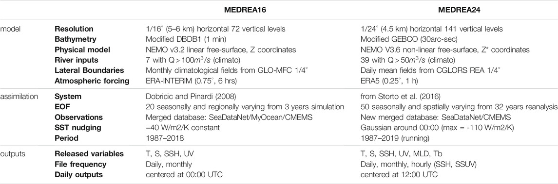
TABLE 1. Comparison with Previous reanalysis.
The SST data used to correct the heat fluxes in the numerical model are L4 interpolated fields from CMEMS (CMEMS product name is SST_MED_SST_L4_REP_OBSERVATIONS_010_021). This is an optimally interpolated satellite-based estimate of the foundation SST in the Mediterranean Sea and adjacent North Atlantic box over a 1/24° resolution grid. This product is built from a consistent reprocessing of the level-3 (merged multi-sensor, L3) climate data record provided by the ESA Climate Change Initiative (CCI) and Copernicus Climate Change Service (C3S) initiatives, but also includes an adjusted version of the AVHRR Pathfinder dataset version 5.3 to increase the input observation coverage (Buongiorno Nardelli et al., 2013; Pisano et al., 2016). This product is the result of a merge of several sensors documented extensively in its documentation (see on CMEMS website).
The 3DVar system described below assimilates the along-track sea level anomalies (SLA) from satellite altimetry. This reprocessed data over the European region, using all available satellites, is also provided through CMEMS project by the DUACS multimission altimeter data processing system (CMEMS product name is SEALEVEL_EUR_PHY_L3_REP_OBSERVATIONS_008_061). The product provides the different corrections applied to the data as separate variables which allows us to choose not to apply the Dynamic Atmospheric Correction (DAC) since the NEMO configuration uses a free surface equation that accounts for the atmospheric pressure effect (Dobricic et al., 2012; Oddo et al., 2014). It was also chosen to use unfiltered SLA to avoid the filtering of physical signal and let the assimilation system handle the resulting noise. For each track and each pass of the satellite the mean bias over the whole uninterrupted track between the observation and the model value is removed from the innovation. This enables to avoid lingering large scale atmospheric effects and other uncorrected signal.
The system also assimilates in-situ temperature and salinity profiles for the whole period. These profiles come from CTD (“Conductivity Temperature and Depth”, ship measurements), XBT (Expendable bathythermograph) and ARGO floats (profiling floats). They are obtained by merging the data from CMEMS historical NRT in-situ observations (CMEMS product name is INSITU_GLO_NRT_OBSERVATIONS_013_030) into the database of in-situ observations from SeaDataNet (https://www.seadatanet.org/). We found out that both datasets were missing some good observations and by merging the two we obtain a larger database (around 30% more data after preprocessing). The merging procedure removes profiles from CMEMS that were already in SeaDataNet. The resulting database is then pre-processed before the observations are introduced into the system. First, only the physical profiles for ARGO (first profile of the day in the CMEMS database) are kept. From this sensor, profiles with gap in thermocline (more than 40 m in the first 300 m) are removed. Only data with quality check value of 1 (good data) are retained and temperature values must be within (0–35)°C and salinity within (0–45) PSU. If the data has no recognized type, it is considered a CTD if there are salinity values in the profile, XBT otherwise. For CTD data, only ascending profiles are selected. All measurements above 2 m are discarded (for ARGO and XBT). 17% of data is rejected with the above pre-processing. Finally, a vertical subsampling is performed to keep no more than 3 observations per model level.
For the evaluation of the performance of the reanalysis, assimilated observations were compared to the model outputs as quasi-independent observations. Fully independent observations take the form of fixed mooring time series of temperature and salinity as well as tide gauges measurements. This data comes from the European Marine Observation and Data Network (EMODnet, https://emodnet.ec.europa.eu/). Interpolated 2D daily maps of satellite altimetry are also used in the validation to generate the Eddy Kinetic Energy (EKE) maps and compare them to the reanalysis outputs. These maps are obtained from the CMEMS database (CMEMS product name is SEALEVEL_MED_PHY_L4_REP_OBSERVATIONS_008_051) and are estimated by an optimal interpolation method, merging the measurements from the different available altimeter missions.
The OceanVar data assimilation scheme (Dobricic and Pinardi, 2008) is a variational scheme in which the slowly evolving vertical part of temperature and salinity background error covariances is represented by monthly climatological spatially varying empirical orthogonal functions (EOFs), whilst their horizontal part is assumed to be Gaussian isotropic depending only on distance. In the horizontal direction, we apply the isotropic covariances, because we assume that, due to the large variability of parameters at the high horizontal resolution of the model, it could become very difficult to correctly estimate the complex structures of the horizontal background error covariances by a set of climatological EOFs.
In the 3DVar formulation of the data assimilation, we need to minimize a cost function J that represents the distance between the analysis and both the background state (the physical model outputs) and the observations. The incremental formulation of J is:
where B and R are the background- and observation-error covariance matrices. δx = x − xb with x the ocean state, i.e., the analysis at the minimum of J, and xb the background state. In our formulation, we want to correct temperature, salinity and sea surface height so the ocean state is x = (T, S, η). H is the observation operator and d is the innovation vector (background minus observations in the observation space).
We assume that B can be written in the form B = VVT. Then using the change of variable δx = Vv, the cost function can be written (Control Variable Transformation or CVT):
The CVT provides a way to represent error covariances without explicitly constructing the background-error covariance matrix B. The gradient of the cost function becomes:
The matrix V is decomposed into a series of linear operators as follows:
In Equation 4 the linear operator VV transforms coefficients which multiply vertical EOFs into vertical profiles of temperature and salinity defined at the model vertical levels, VH applies horizontal covariances on fields of temperature and salinity, Vη covaries the SSH increments with three-dimensional salinity and temperature increments using dynamic height formulation (Cooper and Haines, 1996; Storto et al., 2011).
In the formulation of Equation 1, the fully nonlinear observation operator is used only once for computing the initial departures employing the background fields closer to the observation time (FGAT). The tangent-linear model is used for updating the cost function at each iteration according to the new model state, while the adjoint model is used for mapping the new observation departures back onto the control space for the gradient computation. Their linearization is performed around the background fields closer to the observation time. A hybrid-parallel version of OceanVar (similarly to Cipollone et al., 2020) with a standard formulation of the cost function (Eq. 1 and Eq. 2) without other penalty terms is used.
The vertical covariance operator VV is composed of 50 monthly climatological trivariate EOFs that were computed from the daily anomalies of a previous 32 years run with data assimilation. These EOF are computed at each model grid point and we apply a vertical localization (Gaussian with length scale of 800 m) to avoid spurious covariances between upper and lower layers. In order to have more independent profiles, we selected only profiles every 5 days. This means that, for example, we use 192 profiles at each location to compute the EOF of the month of January (6 days in each of the 32 years). 50 EOF are enough to reproduce the variability at more than 99.9% (not shown). As an illustration, Figure 2 presents the correlation between different levels of the model and different variables that come from the 50 EOF computed for two different months at two different points of the Mediterranean Sea. The effect of the vertical localization is visible as the correlations tend towards zero between two levels that are far apart. In the first location and month, temperature and salinity have negative correlation in the first 40 model levels while the second location has a positive correlation for the first 20 model levels. The same procedure adopted for covarying T and S can be extended to include SSH. The correlation obtained in this case is also here plotted (right panels) as information. It is worth stressing that this correlation is purely empirical and can therefore potentially destroy the hydrostatic equilibrium of the water column. In the current version of the reanalysis, we covaried SSH with T and S through a balance operator that will be discussed later. Developments are in place to include also the unbalanced part (from the EOF) in the next version of the system.
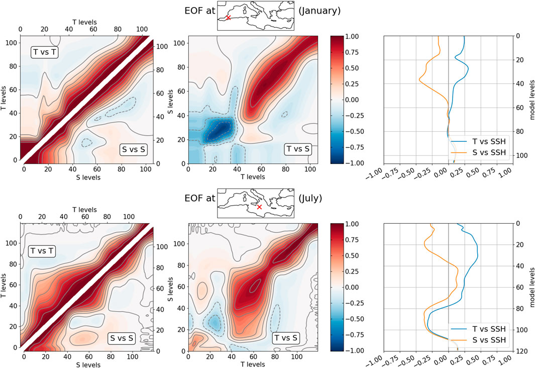
FIGURE 2. Examples of correlations computed from the EOF on two model grid points for two different months: January on the upper row and July on the lower row. On each row, the left is the correlation obtained between temperatures (and salinities) at different model levels, the center is the correlation between temperature and salinity at different levels and the right is the correlation between SSH and temperature (or salinity).
The second component of the V operator is the recursive filter (VH). This filter follows the design of Dobricic and Pinardi (2008) to propagate the information of the increment in the horizontal direction. We use a correlation length scale of 15 km which represents the typical Rossby radius of the basin and perform 4 iterations of the first-order filter that are sufficient to reproduce the Gaussian shape with a good degree of accuracy (Dobricic and Pinardi, 2008; Farina et al., 2015).
Finally, the last operator is the dynamic height operator Vη. This operator is used to get the SLA anomaly from the temperature and salinity profiles and vice-versa. The method, described in Storto et al. (2011), uses the local hydrostatic adjustment that relies on the vertical integration of density from a “no motion” level where it is assumed that the horizontal pressure gradient is almost zero. This level is fixed at 1,000 m in our configuration and consequently SLA observations in regions where the maximum depth is less than 1,000 m are discarded.
For the covariance error matrix of observations, we assume that the observations are uncorrelated and thus the matrix is diagonal. The information needed is then the variance of the observation error. This error eo is the sum of the measurement or instrument error eμ and the representativity error er that is made when we put the continuous ocean into a gridded field: eo = eμ + er. While the former is relatively easy to get from sensor manufacturers, the second is more difficult as it depends on the model grid and local dynamics. To estimate the full observation error, we then used the method prescribed in Desroziers et al. (2005). This iterative method estimates the observation errors by using the innovations and residuals from repeated runs of the system. We first prescribed the errors used in the previous system and then iterated using errors estimated from the formulae in Desroziers et al. (2005). When the errors are no longer changing (3 iterations in our case), we have obtained an estimation of eo.
Figure 3 presents the final vertical profile of the observation error standard deviation that we obtained for the different platforms that we assimilate (XBT, CTD, and ARGO floats). We apply these profiles of error in the whole domain, meaning that there is no space dependency and only seasonal and vertical dependency. For the temperature, the error profiles are similar with a strong seasonal variability in the thermocline region. We can note that the salinity error for the CTD is much higher in the surface than ARGO error. This is because CTD observations are much more coastal and model salinity in these locations can diverge strongly from observations due to rivers outflow. The observations error then reflects this discrepancy.
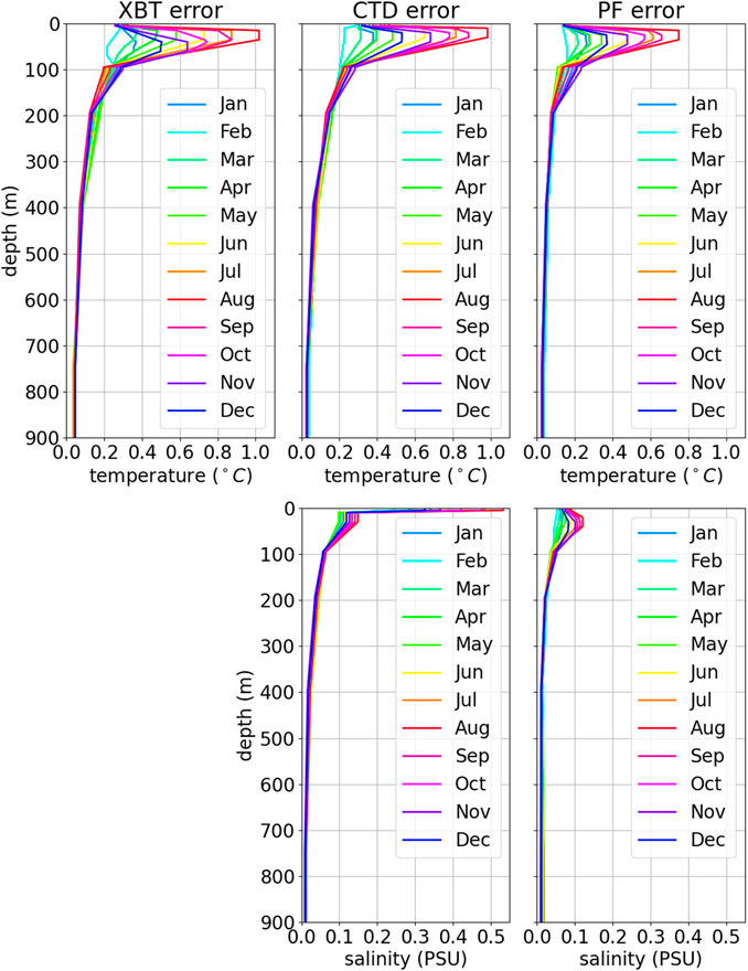
FIGURE 3. Insitu error profiles used in the data assimilation. Top panels are temperature errors while bottom panels are salinity. Errors for XBT, CTD and ARGO floats are respectively plotted on the left, center and right columns.
For the SLA assimilation, the observation error is fixed to be constant in time and space. The satellites have different instrument error but the differences are assumed to be small and therefore we can use the same error as a first approximation. The value of this observation error is set to 3 cm and was estimated using sensitivity experiments. These experiments were performed for 2 years (2004–2005) and the analysis global statistics as well as the study of well documented mesoscale events resulted in the value of 3 cm and the use of unfiltered SLA variable in the dataset proving to better represent the regional features with lower error. The estimation from the formula in Desroziers et al. (2005) confirms that 3 cm is a good guess for the total error.
The system implements a background quality check procedure that rejects observations whose square departure exceeds a certain number of times the sum of the observational and background-error variances. For the ith observation, the observation retention criterion reads
with
To evaluate the quality of the reanalyses, the daily model outputs have been bi-linearly horizontally interpolated at each observational position considering the four closest model grid points and then linearly vertically interpolated. These interpolated outputs (Ymodel) are then compared to the observations measurements (Yobs) and we compute the Root Mean Square Difference (RMSD) and bias as:
The observations used in the validation assessment are mostly from the same datasets used for the data assimilation. However, since the assimilation is performed at the end of the day, the evaluation is done before each observation is assimilated (the increment is applied on the following day) and thus it can be considered as quasi-independent.
To provide another reference, a hindcast, run of the numerical model without data assimilation or SST relaxation, is also presented (hereafter called MEDHIND24).
The time evolution of the RMSD and bias of the comparison with SST observations from satellites is shown in Figure 4. For the SST diagnostics, the observations are not fully independent as the SST observations are used to correct the heat fluxes in NEMO (see Numerical Model).
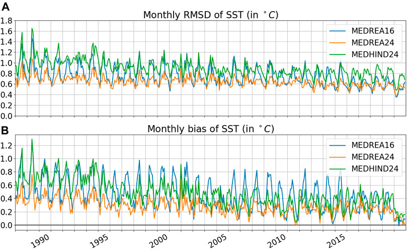
FIGURE 4. Monthly RMSD (A) and bias (B) of SST (in °C) for the two reanalyses and the hindcast when compared to satellite SST. The first model layer is used for the model SST.
Both MEDREA16 and MEDREA24 present a positive bias, meaning that the first layer of the model is warmer than the SST observations. This bias is positive in the whole basin (not shown). However, it is decreasing with time as the model gets closer to the observed SST values. The RMSD also decreases with time as a consequence of the diminishing bias. The new reanalysis has consistently a smaller bias and RMSD than MEDREA16 in summer when the difference is the largest. The RMSD value over the whole period is 0.78°C for the previous reanalysis and 0.65°C for the new one. This improvement is attributed to the atmospheric forcing fields (ERA5) that perform better in the region compared to the previous version (ERA-INTERIM). The hindcast SST RMSD and bias is higher than the reanalysis showing that the relaxation to the SST observations is having the intended effect.
In this section, we compare the model outputs with temperature profile measurements from CTD, XBT, and ARGO floats. These observations are assimilated but, as mentioned before, their values are compared to the model daily outputs before the observation is assimilated.
The time evolution of the monthly RMSD for different layers of the whole Mediterranean domain is reported in the of Figure 5A. The RMSD is highest in the 10–100 m depth layer with highly seasonal variability and largest values in summer. The shallow layer (0–10 m) also presents a seasonal signal with high values in summer. This is clearer in the most recent years (after 2010) when there is a more constant time coverage of the observations due to the ARGO floats. Deeper layers have very little seasonality and also present a very low variability after 2010. MEDREA24 performs consistently better than MEDREA16, especially at depth and in the most recent years. A possible reason for this improvement is that, in MEDREA16, there were less assimilated profiles and virtually no assimilated observation below 1,000 m.
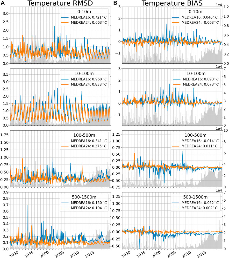
FIGURE 5. Monthly temperature RMSD (A) and bias (B) (in °C) for the two reanalyses and the hindcast when compared to observed profiles for different layers. The values of RMSD/bias for the whole period are indicated in the legend. The shaded area represents the number of observations for each month (axis is on the right). Note the different y-axis in the different layers.
Looking at the bias in Figure 5B , this improvement at depth is associated to a reduction of a negative bias. This figure also shows less temporal variability of the bias in MEDREA24 in all the layers confirming the better skill of this version. In this reanalysis there is no persistent bias that we can detect at any layer. We note that in January 2000, there is a spike in the RMSD with a corresponding negative bias. This comes from “bad observations” where a whole campaign of observations in the Western Mediterranean is present in the observation dataset but the values of temperature (around 28°C at the surface) suggest that these observations were made in summer.
A more detailed view of the vertical comparison and the comparison with the hindcast outputs is offered in the top panels of Figure 7. It clearly shows the improvement of the new reanalysis compared to MEDREA16 in temperature at all depths, especially in the deep ocean. Below 200 m, the remaining bias is largely reduced in MEDREA24. The hindcast results show that the reduction of the bias can be largely attributed to data assimilation. The maximum error is found in the thermocline, at around 30 m, in both reanalyses and corresponds to the peak in summer in the time evolution. It is hypothesized that this error is due to an imperfect vertical mixing scheme that results in errors in the position of the thermocline during this season. The bias maximum is slightly below the depth of the maximum error, at around 50 m, and positive, indicating a possible overestimation of the mixed layer thickness as the temperature is stratified during summer period and the water column is well mixed during winter season. As seen in Figure 5, this bias is however greatly reduced in the more recent years. Between 20 and 200 m, both reanalyses present a resulting positive bias due to the summer overestimation of the temperature shown in the previous picture. In the upper layers, the error is very similar between the two experiments but the bias has an opposite sign. This discrepancy should come from data assimilation or more likely the heat flux correction by the observed SST since the hindcast shows a similar bias as MEDREA16. Indeed, in the previous section, the SST from satellite was consistently lower than the model SST resulting in relaxation toward cooler SST. The atmospheric forcing could have also an impact as the atmospheric fields are different with MEDREA24 using the more recent hourly fields from ERA5 whereas MEDREA16 uses 6-hourly fields from ERA-INTERIM. An internal evaluation of the ERA5 fields showed lower values of 2 m temperature in summer and an increase of the averaged cloud cover all year over the Mediterranean in comparison with ERA-Interim. This can explain part of the reduction of the positive bias in the surface layers as, which is highest in summer (see Figure 5).
The daily model estimates are here compared to the salinity profiles from CTD surveys and ARGO floats. The monthly time evolution of the RMSD for different layers is shown in Figure 6A. The highest error is found in the upper layers as 0.47 PSU and 0.58 PSU for the new and the old reanalysis, respectively. At all the layers, there is a strong variability in the early years that is reduced significantly in the ARGO era when there is a much better coverage of the region. The error is consistently decreased with the new reanalysis with the largest improvement in the deep layers.
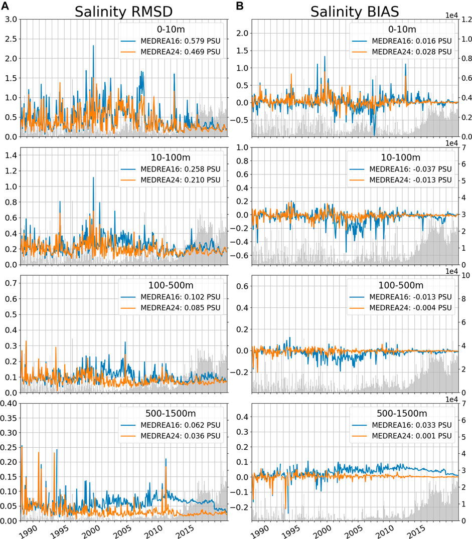
FIGURE 6. Monthly salinity RMSD (A) and bias (B) (in PSU) for the two reanalyses and the hindcast when compared to observed profiles for different layers. The values of RMSD/bias for the whole period are indicated in the legend. The shaded area represents the number of observations for each month (axis is on the right). Note the different y-axis in the different layers.
Bias evolution (Figure 6B) confirms the decrease of variability in the later years. Below 50 m, the increase of the error of the MEDREA16 is shown to be related to a positive salinity bias. On average, the bias is improved in MEDREA24 except in the near surface where the average value is higher. However, at the surface, the bias of the new reanalysis does not appear to be consistent and fluctuates in time pointing that this average value may not be significant.
The vertical distribution of these diagnostics is specified in the bottom panels of Figure 7, with the hindcast values added for comparison. They confirm that the error is consistently reduced at all depth. The bias is largely reduced at depth too, especially below 1,000 m where the previous reanalysis had a bias. Increased vertical resolution and a more realistic representation of the freshwater inputs, achieved thanks to the increased number of rivers (from 7 to 39, Delrosso 2020) implemented in the new reanalysis, the use of higher spatial and temporal precipitation data, and the improved nesting in the Atlantic Ocean by means of daily open boundary conditions from a global model (instead of monthly climatological fields), could have concurred in the improved representation of the salt budget of the basin. The hindcast salt content (Figure 7) still presents some bias at depth and these are corrected by the assimilation of profiles. In the case of MEDREA16, very few observations were assimilated below 1,000 m. We notice that in the first 10 m, the previously mentioned (see Figure 6) larger positive bias in the new reanalysis. Horizontal maps of the bias (not shown) seem to indicate that it is related to an underestimation of the low salinity near the rivers and may be related to the non-zero salinity imposed for the river inflow.
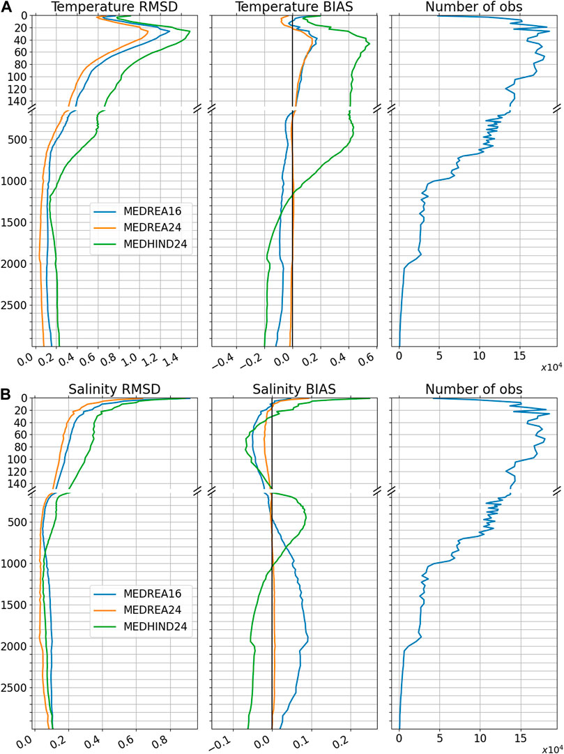
FIGURE 7. Vertical temperature [(A), in °C] and salinity [(B), in PSU] diagnostics for the two reanalyses and the hindcast when compared to observed profiles for the whole period (1987–2019). The diagnostics were computed on the model layers and the right panel present the number of observations used. The vertical scale is increased on the plot for the first 150 m to better see the upper layers values.
The monthly RMSD with SLA observations is reported in Figure 8. Again, this is a quasi-independent evaluation as these observations are ingested by the system to correct itself after the evaluation is done.
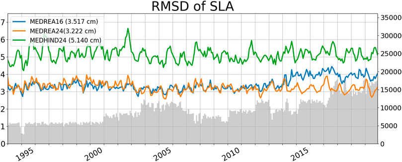
FIGURE 8. Time evolution of the monthly RMSD of SLA (in cm) for the two reanalyses and the hindcast. The SLA is taken where the ocean is deeper than 1,000 m as it is done for the assimilation. In grey is the number of observations used for this diagnostic.
Both reanalyses boast similar skill with respect to this observational dataset with an error value of 3.2 cm until 2013. Then they start to diverge and the new reanalysis MEDREA24 continues with this behavior whereas MEDREA16 shows a decrease of skill. This is due to the fact that the older reanalysis did not assimilate all the satellites present in this period. Over the whole period, the new reanalysis presents a 8% decrease of the error (from 3.5 to 3.2 cm).
Table 2 presents a summary of the RMSD of the new reanalysis with respect to observations along with the percentage difference compared to the previous reanalysis skill. It highlights the improvement brought by the new reanalysis at least on this particular skill assessment. On the table the RMSD evaluated comparing with fixed moorings surface temperature and salinity and with tide gauges SSH. Considering the moorings temperature and salinity, the new reanalysis does not show significant skill improvements when compared with the previous one. It is to be noted that this comparison is very coastal and near the surface and thus quite limited. Considering the comparison with tide gauges, the reanalysis sea level shows an error of 6.7 cm which is larger than the sea level anomaly error (3.8 cm) computed using altimeter data since tide gauges are located close to the coast but there is an improvement relative to the previous reanalysis (21% decrease of RMSD). In general, the improved skill of the new reanalysis when comparing to fixed and not assimilated data, is mostly due to improvement of the numerical model as the hindcast skill (not shown) is quite similar.
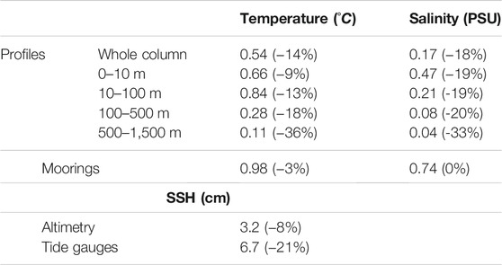
TABLE 2. Summary of estimated RMSD compared to observations for the whole Mediterranean Sea. The value is for MEDREA24 and the percentage in parenthesis is the change from MEDREA16.
The ability of the system to represent climate signals is evaluated looking at the heat content in different layers of the ocean. This heat content, computed as the volume-averaged temperature in different layers from both reanalyses and the hindcast, is presented in Figure 9A showing an overall increase of temperature during the considered period in the whole water column.
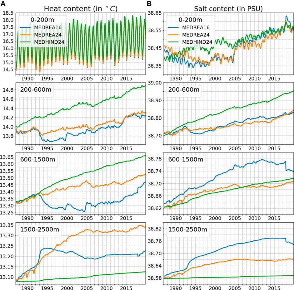
FIGURE 9. Time evolution of heat content [(A), in °C] and salt content [(B), in PSU] in different layers for both reanalyses and the hindcast. These are averaged over the whole Mediterranean Sea.
In the upper 20 m, this signal is mostly dominated by a strong seasonal cycle. The new reanalysis presents a marginally stronger seasonal amplitude (1.30°C vs 1.25°C) with warmer summers. The hindcast has an intermediate seasonal amplitude (1.28°C) with warmer winters, meaning that the assimilation contributes to the cooling of winters. This signal is also modulated by large interannual variability and a positive trend. The interannual variability is similar for all experiments and not negligible and for example, between 1990 and 1992 there is a decrease of 2°C. The standard deviation for the interannual signal is 0.16°C for all the curves. Concerning the trend, we get 0.026°C/year (0.023°C/year) increase of temperature for MEDREA24 (MEDREA16). The hindcast trend at the surface is slightly weaker (0.022°C/year).
In the layer below (200–600 m), the seasonal signal drops completely with an amplitude below 0.01°C for both reanalyses. The new reanalysis presents a steady increase of temperature modulated by some interannual variability. The other reanalysis however saw a larger drop of temperature from 1992 to 1994 followed by a stronger positive trend later. The drop around 1993 is not reproduced in the hindcast. In the end, the computed trend for both is equal to 0.013°C/year over the period while the hindcast presents a trend twice as large.
The decreased temperature in the early 90s is also noticeable in the deeper layer (600–1,500 m) for MEDREA16 although it occurs at a later date (after 1993) and more gradually. In MEDREA24, there is no drop of temperature but the trend is reduced after this period while the hindcast heat content keeps increasing at the same pace. Around the end of the simulation, MEDREA16 catches up with the estimation from the new reanalysis, probably thanks to the assimilated observations. As shown in Figure 5, the new reanalysis estimate is closer to the observations and the previous one had a cold bias. The trends are respectively 0.002°C/year and 0.005°C/year for MEDREA16 and MEDREA24 (the hindcast trend is 0.01°C/year).
In the bottom layer, both reanalyses have first a phase of warming followed by a period of relative stability. However, the new reanalysis warming phase is longer, lasting until around 2005 and there is still some lighter warming afterwards. The hindcast presents a weaker and constant warming in the deep ocean.
The accuracy of the heat content variations in the new reanalysis can be assessed by comparing it to other products. This is done in the CMEMS OMI (ocean monitoring inticators https://marine.copernicus.eu/access-data/ocean-monitoring-indicators) where the heat content deviation from a reference period (1993–2014) integrated over the 0–700 m depth layer is computed for global reanalyses and observation-only based products. This is reproduced in Figure 10 where the estimates from global reanalyses (GLORYS, C-GLORS, ORAS5 and FOAM, from the CMEMS product GLOBAL_REANALYSIS_PHY_001_031) and MEDREA24 are plotted alongside estimates from observation based products (CORA and ARMOR3D). The ensemble mean ocean heat content anomaly time series over the Mediterranean Sea shows a continuous increase in the period 1993–2018 at rate of 1.5 ± 0.2W/m2 in the upper 700 m. After 2005 the rate has clearly increased with respect to the previous decade, in agreement with Iona et al. (2018). The picture confirms that MEDREA24 is well within the ensemble of estimates and is actually the one that is closest to the mean of all products (lowest RMSD).
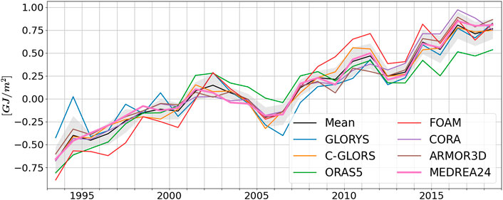
FIGURE 10. Time series of area averaged ocean heat content anomaly in the Mediterranean Sea, and integrated over the 0–700 m depth layer. Time series are based on different data products. The mean profile is in black and the grey shaded area corresponds to the ensemble spread.
The salt content time evolution in different layers for both reanalyses and the hindcast is reported on Figure 9B.
On the first layer, from the surface to 200 m, as with temperature, we observe a seasonal cycle with saltier waters in winter and fresher in summer. However, it accounts for less of the total variability in salt content (58%) than in heat content (97%) in both reanalyses. The salt content is slowly decreasing from 1987 to 2005 when there is a sharp increase followed by a slow increase of salt in the basin. Despite some small differences, the interannual variations are similar in both reanalyses. The hindcast, however, shows a quite different behavior before 2005. This hints that the assimilation of in-situ observations has a large effect in the salt content interannual variability for the upper layers. The trend is respectively 0.007 PSU and 0.005 PSU for MEDREA16 and MEDREA24 reflecting that the older reanalysis had a more pronounced decrease at the start and then increase at the end of the period.
On the layer below, there is no more perceivable seasonal cycle and the signal is dominated by interannual variability. Both timeseries present similar characteristics with a trend of 0.0038 PSU/year (MEDREA16) and 0.0032 PSU/year (MEDREA24). As in the heat content, there is a drop of salinity in 1992 in MEDREA16. This dip is no longer present in the new dataset. It is unclear what was the source of this behavior and therefore why it is not seen in the new reanalysis. As seen in the heat content, the trend for the hindcast is twice as large and the assimilation helps avoiding the non-realistic drifts.
In the deeper layer, the drift in the old reanalysis that we already discussed is evidenced with a trend twice higher (0.004 PSU/year) than in the new reanalysis. This trend was not realistic and is here corrected as shown in the previous section (Figure 7 for example). In 2018, a new initial condition for the extension of the timeseries corrected this bias partially but was not sufficient. For this layer, the hindcast trend is similar to the assimilated run, meaning that the correction of the trend is related to the change in the physical model.
At the bottom of the basin, a similar analysis can be made with the new reanalysis correcting the bottom drift in salinity and the new trend is now 0.0026 instead of 0.0057 PSU/year. Now, the trend of the hindcast is too low compared to the other experiments and this explains the negative bias in the deeper layers found in Figure 7.
The changes in temperature and salinity content also have an impact on the mixed layer depth (MLD) in the basin. MEDREA24 MLD climatology is quite consistent with estimations from observations (see the QUID documentation on the CMEMS website for more details, Escudier et al., 2016). Looking at the mean mixed layer depth in convection areas reveals that the new reanalysis has stronger deep convection than MEDREA16 but also the hindcast (not shown), showing that the corrections of temperature and salinity have a strong impact on this variable. This will be analyzed and described more in depth in a further study.
The average circulation of MEDREA24 is presented in Figure 11 on the surface and on the sub-surface (200–300 m). It shows that the new reanalysis is able to correctly reproduce the main currents and circulation. A full description of the circulation can be found in Pinardi et al. (2015) but here we will point out the main features.
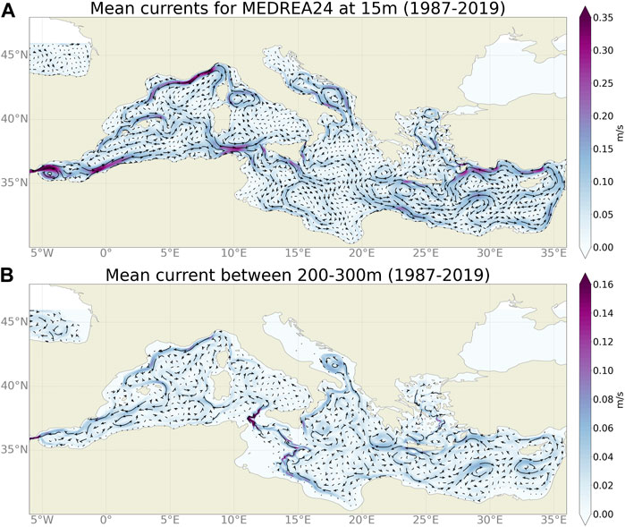
FIGURE 11. Average currents from MEDREA24 at 15 m (A) and between 200–300 m depth (B) for the period 1987–2019.
At the surface, the water coming from the Atlantic flows through the Gibraltar Strait and forms the two Alboran gyres in the Alboran Sea. The Eastern gyre is smaller in amplitude as it is only semi-permanent. Then the Algerian current that transports this water along the African coast is strong and narrow in the western part and less intense and defined in the eastern part due to the high mesoscale activity and the large anticyclonic eddies that modulate the mean current. South of Sardinia, the current is joined by a current coming from the North along the Sardinia western coast and flows eastward along the Tunisia coast toward the Tyrrhenian Sea. A part of this current then continues eastward along the Northern Sicilian coast, another loops around the South-Western Tyrrhenian Gyre and the rest crosses the Sicily Strait. From the first part, a relatively strong current flows on the surface through the Messina Strait between Sicilia and Italy’s mainland while there is a weak circulation northeastward along the Italian coast. In this Tyrrhennian Sea, the other known gyre is the Northern Tyrrhenian Gyre (Artale et al., 1994) which is strongly reproduced in the model. From this gyre, the waters passing through the Corsica channel join the Gulf of Lion gyre and more specifically the northern part of it, the Northern current. This is a relatively strong current that follows the Southern coast of France and even extends along the Spanish Catalan coast, which is better reproduced in this version of the reanalysis. The Balearic current forms the beginning of the return part of the gyre flowing along the Northern coast of the Balearic Islands. In the Ibiza channel, there should be two current, one northward and the other southward (Heslop et al., 2012) and the reanalysis only has a northward current joining the Balearic current. Back at the Sicily Strait, the Algerian current branches into two currents, one southward (Sicily Strait Tunisian Current) and the other eastward along the Southern Sicily coast (Atlantic Ionian Stream, AIS). Both currents then meet a large anticyclonic gyre in the Southern part of the Ionian Sea (Sirte gyre in Pinardi et al., 2015). A part of the AIS meanders northward until both branches join into the Cretan Passage Southern Current (CPSC). North of this current, the Pelops Eddy (or Pelops Gyre) and the Western Cretan Eddy (Mkhinini et al., 2014) are represented. The CPSC then goes northward to become the Mid-Mediterranean Jet (MMJ, Golnaraghi and Robinson 1994) to form the Mersa Matruh gyre. The Southern Levantine current (SLC) follows the African coastline, bordering the Shikmona gyre in the eastern part of the basin and going northward around Cyprus to become the Asia Minor Current. This current turns southward when arriving at Crete forming the Rhodes gyre on the east and the IeraPetra gyre on the west. In the Aegean Sea, the main currents form a cyclonic circulation around the sea.
The subsurface circulation (bottom of Figure 11) corresponds to the circulation of the Levantine Intermediate Water. Starting from the Levantine Sea where the LIW is formed, the Shikmona and Mersa-Matruh gyres are also well defined. The flow follows the surface currents northward along the middle eastern coast and then westward like the Asia Minor current. Then both the Pelops Eddy and the Western Cretan Eddy will modulate the western propagation of the LIW. Some of the current goes northward to the Adriatic Sea and then south-westward along the Italian coast to the Sicily coast. The rest is flowing southward then westward on a coastal current that follows the Sirte gyre southern part. Both branches then join in the Sicily Strait where the highest velocities (0.2 m/s) are reached. The LIW is then advected towards the southern coast of France either in the Tyrrhenian Sea or along the western coast of Sardinia and Corsica. The Northern Current then propagates these waters south-westward to the Balearic Sea where they either turn east along the Balearic Current to circle around the Balearic Islands or they flow through the Ibiza Channel. Then they continue westward along the Spanish coast to reach the Gibraltar Strait.
It is difficult to evaluate quantitatively the differences in the mean circulation with respect to the previous reanalysis and an in-depth analysis is outside of the scope of this section. However, we can highlight some improvements in the surface (see Figure 3 of Pinardi et al., 2015) such as the Algerian current that is stronger and closer to the coast, the Northern current that reaches further in the Balearic Sea, the clearer separation in three branches south of Sicily (with current coming from the now open Messina Strait), a better representation of the Western Cretan Eddy or the Mersa Matruh gyre that has a better defined structure. As for the subsurface circulation, less is known about it but we can note that the gyres in the Eastern basin are more clearly defined and, in the Western basin, the Northern current goes further west also at depth.
Another view of the surface currents is presented in Figure 12. Here the averaged Sea Surface Height (SSH) over the altimetry time period is shown with the resulting geostrophic currents computed from the geostrophic equilibrium. In the figure, the Mean Dynamic Topography (MDT) from Rio et al. (2014) is plotted below as “reference”. This MDT is computed using a numerical model as a first guess and then combining it with all the available observations of the currents. This plot allows to clearly see the circulation and especially the various gyres that were discussed above. The modelized mean SSH is smoother than the MDT but displays very similar structures. Some differences can be found in both circulations such as the situation in the Aegean Sea where the model has a more accurate representation of the circulation (see Olson et al., 2007 for an independent estimation).
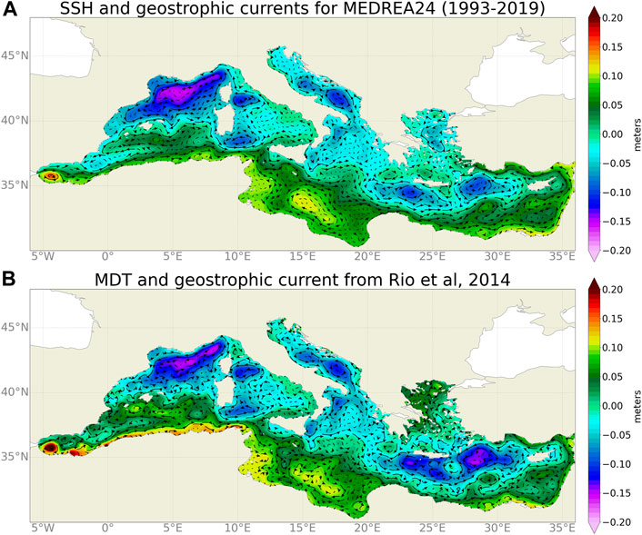
FIGURE 12. Mean SSH and associated geostrophic currents for MEDREA24 during the period 1993–2019 (A) and Mean Dynamic Topography (B) used for the SLA assimilation. A global constant has been removed in the basin in both plots.
To characterize the mesoscale activity in the new reanalysis, the average Eddy Kinetic Energy (EKE) over the whole period is represented in Figure 13. This EKE was computed from the SSH of the model as well as the SSH from altimetry maps. It allows to estimate the skill of the model keeping in mind the flaws and shortcomings of the altimetry interpolated maps. Indeed, these maps come from an optimal interpolation and therefore the fields are smoothed. In the Alboran Sea, the reanalysis has an eddy activity at the entrance from the Gibraltar Strait and along the entering current. This higher mesoscale activity close to the coast was also found in a high resolution regional model of the Alboran Sea (Peliz et al., 2013). Altimetry maps do not have the capability to resolve these small coastal eddies. In the Algerian current, similar levels of EKE is found in both datasets with the reanalysis having more coastal mesoscale activity. The Northern part of this sub-basin highlights stronger differences with almost no activity in the altimetry maps whereas the reanalysis shows mesoscale variability along the Northern current and in the Balearic Sea. The explanation for this is that the Rossby radius is smaller there than in the Southern part and thus the eddies are smaller (Escudier et al., 2013, 2016). Filtered and interpolated altimetry maps are thus not able to reproduce these structures. In the Tyrrhenian Sea, the EKE is highest around the Northern Tyrrhenian Gyre in both maps but, in the model, the current flowing north of Sicily also presents a stronger EKE. The model EKE in the Adriatic Sea contours the surface currents while the altimetry maps show no mesoscale activity. Here again, the smaller eddies due to a smaller Rossby radius can be the reason behind this discrepancy. In the Eastern part of the basin, the model differs from the remote sensing data with higher EKE along the coast and the coastal surface currents that compose the main cyclonic circulation. The strongest mesoscale activity is found around the Iera-Petra eddy location for both. However, in the altimetry product, variations in the eddy intensity are stronger and there is a clear trace in the EKE. This means that the reanalysis is not capable of fully reproducing the variability of this eddy. The Aegean Sea is a region that is difficult to observe with altimetry due to the high density of islands, therefore the higher EKE in the model is expected. Overall, the model and the observation datasets present similar patterns and most differences can be explained by the fact that the model can resolve smaller scales than the interpolated maps of altimetry.
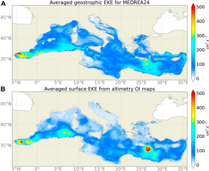
FIGURE 13. Average geostrophic EKE (in cm2. s−2) computed from MEDREA24 SSH (A) and altimetry interpolated maps (B) for the period 1987–2019.
This paper describes a new reanalysis of the Mediterranean Sea that was produced in the framework of CMEMS. The new, higher resolution reanalysis shows good skill in the diagnostics performed and represents a significant improvement with respect to the previous version. The positive surface bias in SST is reduced, as well as the negative bias of temperature in the deeper layers. Concerning salinity, the biases below 500 m are now largely removed. The RMSD when compared to observations is reduced for all variables. The heat content evolution is consistent with observations and other estimates from global models. The surface and sub-surface currents correspond to previous knowledge and the surface EKE is comparable to what is observed with satellite altimetry.
There is still some bias observed in the comparison with satellite SST, even though it is reduced in the new version. This positive bias however is not present in the upper layers when compared to in-situ temperature profiles where it is instead negative. This discrepancy hints that the observed profiles are underestimated in the assimilation and that they do not agree with satellite SST. This issue with SST could come from a difference between the model SST we use, the model first layer temperature value, and the SST from satellite observations which is the night SST, so-called foundation SST. These may not be exactly the same and then introduce some biases in temperature at the surface.
The evaluation of the system is mainly done with the same in-situ observation dataset that was prepared for the assimilation. However, as mentioned, the model is evaluated before the observation is ingested. We can mention that all the diagnostics were also performed with a different database (EN4, Good et al., 2013) and the results are the same, confirming that the assessment does not depend on the specific dataset used. Completely independent observations are difficult to find as we want to assimilate all the good quality available observations. The comparison with fixed moorings shows relatively high errors for these coastal and sparse measurement and no difference between the two reanalyses. Comparisons with drifters can be made but these have to be treated carefully and some high order diagnostics such as presented in Bouffard et al. (2014) are outside of the scope of this paper.
Concerning the increased error in temperature around 30 m depth, an issue which was also present in the previous version, it is believed to be related to the vertical mixing in the model. Part of this error has been corrected but is still the highest error in temperature. The step forward to improve the model will then be to use a better parametrization of the vertical mixing and the introduction of tides (barotropic and internal) that may affect this process.
This new reanalysis offers a new estimate, more accurate, of the Mediterranean Sea circulation and characteristics. We have shown that its heat content is consistent with other analysis and that the higher resolution allowed to better reproduce the eddy kinetic energy of the geostrophic velocity field with respect to altimetry. The salinity in the deep layers has been corrected and corresponds more closely the observed values. In the future, this reanalysis could be used to study processes such as the overturning circulation or the deep convection in the different basins (i.e. Pinardi et al., 2019; Somot et al., 2016) as well as initial and boundary conditions for nested modeling studies at sub-regional scales.
The original contributions presented in the study are included in the article/Supplementary Materials, further inquiries can be directed to the corresponding author.
RE performed the computation of the reanalysis and its assessment. The other authors contributed to the design of the system. RE wrote the first draft of the manuscript. All authors contributed to manuscript revision, read, and approved the submitted version.
This work was supported by CMEMS Med-MFC (Copernicus Marine Environment Monitoring Service–Mediterranean Marine Forecasting Centre), Mercator Ocean International Service.
The authors declare that the research was conducted in the absence of any commercial or financial relationships that could be construed as a potential conflict of interest.
The reviewer CY declared a past co-authorship with one of the authors SM to the handling Editor.
All claims expressed in this article are solely those of the authors and do not necessarily represent those of their affiliated organizations, or those of the publisher, the editors and the reviewers. Any product that may be evaluated in this article, or claim that may be made by its manufacturer, is not guaranteed or endorsed by the publisher.
Adani, M., Dobricic, S., and Pinardi, N. (2011). Quality Assessment of a 1985–2007 Mediterranean Sea Reanalysis. J. Atmos. Oceanic Technol. 28, 569–589. doi:10.1175/2010JTECHO798.1
Artale, V., Astraldi, M., Buffoni, G., and Gasparini, G. (1994). Seasonal Variability of Gyre-Scale Circulation in the Northern Tyrrhenian Sea. J. Geophys. Res. Oceans 99, 14127–14137. doi:10.1029/94JC00284
Bethoux, J., Gentili, B., Morin, P., Nicolas, E., Pierre, C., and Ruiz-Pino, D. (1999). The Mediterranean Sea: a Miniature Ocean for Climatic and Environmental Studies and a Key for the Climatic Functioning of the north atlantic. Prog. Oceanography 44, 131–146. doi:10.1016/S0079-6611(99)00023-3
Bouffard, J., Nencioli, F., Escudier, R., Doglioli, A. M., Petrenko, A. A., Pascual, A., et al. (2014). Lagrangian Analysis of Satellite-Derived Currents: Application to the north Western Mediterranean Coastal Dynamics. Adv. Space Res. 53, 788–801. doi:10.1016/j.asr.2013.12.020
Buongiorno Nardelli, B., Tronconi, C., Pisano, A., and Santoleri, R. (2013). High and Ultra-high Resolution Processing of Satellite Sea Surface Temperature Data over Southern European Seas in the Framework of Myocean Project. Remote Sensing Environ. 129, 1–16. doi:10.1016/j.rse.2012.10.012
Carton, J. A., and Santorelli, A. (2008). Global Decadal Upper-Ocean Heat Content as Viewed in Nine Analyses. J. Clim. 21, 6015–6035. doi:10.1175/2008JCLI2489.1
Cipollone, A., Storto, A., and Masina, S. (2020). Implementing a Parallel Version of a Variational Scheme in a Global Assimilation System at Eddy-Resolving Resolution. J. Atmos. Oceanic Technol. 37, 1865–1876. doi:10.1175/JTECH-D-19-0099.1
Clementi, E., Pistoia, J., Delrosso, D., Mattia, G., Fratianni, C., Storto, A., et al. (2017). “A 1/24 Degree Resolution Mediterranean Analysis and Forecast Modeling System for the Copernicus marine Environment Monitoring Service,” in Eight EuroGOOS International Conference, Bergen, Norway, October 3–5, 2017.
Cooper, M., and Haines, K. (1996). Altimetric Assimilation with Water Property Conservation. J. Geophys. Res. Oceans 101, 1059–1077. doi:10.1029/95JC02902
Delrosso, D. (2020). Numerical modelling and analysis of riverine influences in the Mediterranean Sea. Ph.D. thesis, Alma Mater Studiorum Università di Bologna. Bologna, Italy: Dottorato di ricerca in Geofisica. doi:10.6092/unibo/amsdottorato/9392
Demiraj, E., Bicja, M., Gjika, E., Gjiknuri, L., Gjoka Mucaj, L., Hoxha, F., et al. (1996). Implications Of Climate Change for the Albanian Coast. Tech. Rep. Athens, Greece: United Nations Environment Programme.
Desroziers, G., Berre, L., Chapnik, B., and Poli, P. (2005). Diagnosis of Observation, Background and Analysis-Error Statistics in Observation Space. Q. J. R. Meteorol. Soc. 131, 3385–3396. doi:10.1256/qj.05.108
Dobricic, S., Dufau, C., Oddo, P., Pinardi, N., Pujol, I., and Rio, M.-H. (2012). Assimilation of Sla along Track Observations in the Mediterranean with an Oceanographic Model Forced by Atmospheric Pressure. Ocean Sci. 8, 787–795. doi:10.5194/os-8-787-2012
Dobricic, S., and Pinardi, N. (2008). An Oceanographic Three-Dimensional Variational Data Assimilation Scheme. Ocean Model 22, 89–105. doi:10.1016/j.ocemod.2008.01.004
Dufau-Julliand, C., Marsaleix, P., Petrenko, A., and Dekeyser, I. (2004). Three-dimensional Modeling of the Gulf of Lion’s Hydrodynamics (Northwest Mediterranean) during January 1999 (Moogli3 experiment) and Late winter 1999: Western Mediterranean Intermediate Water’s (Wiw’s) Formation and its Cascading over the Shelf Break. J. Geophys. Res. Oceans 109. doi:10.1029/2003JC002019
Escudier, R., Bouffard, J., Pascual, A., Poulain, P. M., and Pujol, M. I. (2013). Improvement of Coastal and Mesoscale Observation from Space: Application to the Northwestern Mediterranean Sea. Geophys. Res. Lett. 40 (10), 2148–2153. doi:10.1002/grl.50324
Escudier, R., Clementi, E., Omar, M., Cipollone, A., Pistoia, J., Aydogdu, A., et al. (2020). Mediterranean Sea Physical Reanalysis (CMEMS MED-Currents) (Version 1) [Data set]. Copernicus Monitoring Environment Marine Service (CMEMS). doi:10.25423/CMCC/MEDSEA_MULTIYEAR_PHY_006_004_E3R1
Escudier, R., Renault, L., Pascual, A., Brasseur, P., Chelton, D., and Beuvier, J. (2016). Eddy Properties in the Western Mediterranean Sea from Satellite Altimetry and a Numerical Simulation. J. Geophys. Res. Oceans 121, 3990–4006. doi:10.1002/2015JC011371
Estubier, A., and Lévy, M. (2000). Quel schéma numérique pour le transport d’organismes biologiques par la circulation océanique. Note Techniques du Pole de modelisation, Institut Pierre-Simon Laplace, 81.
Farina, R., Dobricic, S., Storto, A., Masina, S., and Cuomo, S. (2015). A Revised Scheme to Compute Horizontal Covariances in an Oceanographic 3d-Var Assimilation System. J. Comput. Phys. 284, 631–647. doi:10.1016/j.jcp.2015.01.003
Fekete, B. M., Vörösmarty, C. J., and Grabs, W. (1999). Global, Composite Runoff fields Based on Observed River Discharge and Simulated Water Balances.
Golnaraghi, M., and Robinson, A. R. (1994). “Dynamical Studies of the Eastern Mediterranean Circulation,” in Ocean Processes in Climate Dynamics: Global and Mediterranean Examples (Springer), 395–406. doi:10.1007/978-94-011-0870-6_17
Good, S. A., Martin, M. J., and Rayner, N. A. (2013). En4: Quality Controlled Ocean Temperature and Salinity Profiles and Monthly Objective Analyses with Uncertainty Estimates. J. Geophys. Res. Oceans 118, 6704–6716. doi:10.1002/2013JC009067
Hamon, M., Beuvier, J., Somot, S., Lellouche, J.-M., Greiner, E., Jordà, G., et al. (2016). Design and Validation of Medrys, a Mediterranean Sea Reanalysis over the Period 1992–2013. Ocean Sci. 12, 577–599. doi:10.5194/os-12-577-2016
Hersbach, H., Bell, B., Berrisford, P., Hirahara, S., Horányi, A., Muñoz-Sabater, J., et al. (2020). The Era5 Global Reanalysis. Q. J. R. Meteorol. Soc. 146, 1999–2049. doi:10.1002/qj.3803
Heslop, E. E., Ruiz, S., Allen, J., López-Jurado, J. L., Renault, L., and Tintoré, J. (2012). Autonomous Underwater Gliders Monitoring Variability at “Choke Points” in Our Ocean System: A Case Study in the Western Mediterranean Sea. Geophys. Res. Lett. 39. doi:10.1029/2012GL053717
Houpert, L., Durrieu de Madron, X., Testor, P., Bosse, A., d’Ortenzio, F., Bouin, M.-N., et al. (2016). Observations of Open-Ocean Deep Convection in the Northwestern M Editerranean S Ea: Seasonal and Interannual Variability of Mixing and Deep Water Masses for the 2007-2013 Period. J. Geophys. Res. Oceans 121, 8139–8171. doi:10.1002/2016JC011857
Hulme, M., Barrow, E. M., Arnell, N. W., Harrison, P. A., Johns, T. C., and Downing, T. E. (1999). Relative Impacts of Human-Induced Climate Change and Natural Climate Variability. Nature 397, 688–691. doi:10.1038/17789
Iona, A., Theodorou, A., Sofianos, S., Watelet, S., Troupin, C., and Beckers, J.-M. (2018). Mediterranean Sea Climatic Indices: Monitoring Long-Term Variability and Climate Changes. Earth Syst. Sci. Data 10, 1829–1842. doi:10.5194/essd-10-1829-2018
Juza, M., Mourre, B., Lellouche, J.-M., Tonani, M., and Tintoré, J. (2015). From basin to Sub-basin Scale Assessment and Intercomparison of Numerical Simulations in the Western Mediterranean Sea. J. Mar. Syst. 149, 36–49. doi:10.1016/j.jmarsys.2015.04.010
Juza, M., Mourre, B., Renault, L., Gómara, S., Sebastián, K., Lora, S., et al. (2016). Socib Operational Ocean Forecasting System and Multi-Platform Validation in the Western Mediterranean Sea. J. Oper. Oceanography 9, s155–s166. doi:10.1080/1755876X.2015.1117764
Kourafalou, V., and Barbopoulos, K. (2003). High Resolution Simulations on the north Aegean Sea Seasonal Circulation. doi:10.5194/angeo-21-251-2003
Le Traon, P. Y., Reppucci, A., Alvarez Fanjul, E., Aouf, L., Behrens, A., Belmonte, M., et al. (2019). From Observation to Information and Users: The Copernicus marine Service Perspective. Front. Mar. Sci. 6, 234. doi:10.3389/fmars.2019.00234
Madec, G., Bourdallé-Badie, R., Bouttier, P.-A., Bricaud, C., Bruciaferri, D., Calvert, D., et al. (2017). NEMO Ocean Engine. Paris, France: Notes du Pôle de modélisation de l\’Institut Pierre-Simon Laplace (IPSL). doi:10.5281/zenodo.1472492
Madec, G., Delecluse, P., Imbard, M., and Levy, C. (1997). OPA, Release 8, Ocean General Circulation Reference Manual Tech. Rep. Technical report 96/xx. LODYC/IPSL, Paris, France.
Malanotte-Rizzoli, P., Manca, B. B., d’Alcala, M. R., Theocharis, A., Brenner, S., Budillon, G., et al. (1999). The Eastern Mediterranean in the 80s and in the 90s: the Big Transition in the Intermediate and Deep Circulations. Dyn. Atmospheres Oceans 29, 365–395. doi:10.1016/S0377-0265(99)00011-1
Maraldi, C., Chanut, J., Levier, B., Ayoub, N., De Mey, P., Reffray, G., et al. (2013). NEMO on the Shelf: Assessment of the Iberia–Biscay–Ireland Configuration. Ocean Sci. 9 (4), 745–771. doi:10.5194/os-9-745-2013
Medoc Group, T., et al. (1970). Observation of Formation of Deep Water in the Mediterranean Sea, 1969. Nature 227, 1037–1040. doi:10.1038/2271037a0
Mkhinini, N., Coimbra, A. L. S., Stegner, A., Arsouze, T., Taupier-Letage, I., and Béranger, K. (2014). Long-lived Mesoscale Eddies in the Eastern Mediterranean Sea: Analysis of 20 Years of Aviso Geostrophic Velocities. J. Geophys. Res. Oceans 119, 8603–8626. doi:10.1002/2014JC010176
Oddo, P., Adani, M., Pinardi, N., Fratianni, C., Tonani, M., and Pettenuzzo, D. (2009). A Nested Atlantic-Mediterranean Sea General Circulation Model for Operational Forecasting. Ocean Sci. 5 (4), 461–473. doi:10.5194/os-5-461-2009
Oddo, P., Bonaduce, A., Pinardi, N., and Guarnieri, A. (2014). Sensitivity of the Mediterranean Sea Level to Atmospheric Pressure and Free Surface Elevation Numerical Formulation in Nemo. Geosci. Model. Dev. 7, 3001–3015. doi:10.5194/gmd-7-3001-2014
Oddo, P., Pinardi, N., and Zavatarelli, M. (2005). A Numerical Study of the Interannual Variability of the Adriatic Sea (2000–2002). Sci. Total Environ. 353, 39–56. Mucilages in the Adriatic and Tyrrhenian Seas. doi:10.1016/j.scitotenv.2005.09.061
Olita, A., Dobricic, S., Ribotti, A., Fazioli, L., Cucco, A., Dufau, C., et al. (2012). Impact of Sla Assimilation in the Sicily Channel Regional Model: Model Skills and Mesoscale Features. Ocean Sci. 8, 485–496. doi:10.5194/os-8-485-2012
Olson, D. B., Kourafalou, V. H., Johns, W. E., Samuels, G., and Veneziani, M. (2007). Aegean Surface Circulation from a Satellite-Tracked Drifter Array. J. Phys. Oceanography 37, 1898–1917. doi:10.1175/JPO3028.1
Pacanowski, R., and Philander, S. (1981). Parameterization of Vertical Mixing in Numerical Models of Tropical Oceans. J. Phys. Oceanography 11, 1443–1451. doi:10.1175/1520-0485
Peliz, A., Boutov, D., and Teles-Machado, A. (2013). The Alboran Sea Mesoscale in a Long Term High Resolution Simulation: Statistical Analysis. Ocean Model. 72, 32–52. doi:10.1016/j.ocemod.2013.07.002
Pettenuzzo, D., Large, W., and Pinardi, N. (2010). On the Corrections of Era-40 Surface Flux Products Consistent with the Mediterranean Heat and Water Budgets and the Connection between basin Surface Total Heat Flux and Nao. J. Geophys. Res. Oceans 115. doi:10.1029/2009JC005631
Pinardi, N., Cessi, P., Borile, F., and Wolfe, C. L. P. (2019). The Mediterranean Sea Overturning Circulation. J. Phys. Oceanography 49, 1699–1721. doi:10.1175/jpo-d-18-0254.1
Pinardi, N., Zavatarelli, M., Adani, M., Coppini, G., Fratianni, C., Oddo, P., et al. (2015). Mediterranean Sea Large-Scale Low-Frequency Ocean Variability and Water Mass Formation Rates from 1987 to 2007: A Retrospective Analysis. Prog. Oceanography 132, 318–332. doi:10.1016/j.pocean.2013.11.003
Pisano, A., Buongiorno Nardelli, B., Tronconi, C., and Santoleri, R. (2016). The New Mediterranean Optimally Interpolated Pathfinder Avhrr Sst Dataset (1982–2012). Remote Sensing Environ. 176, 107–116. doi:10.1016/j.rse.2016.01.019
Raicich, F. (1996). On the Fresh Balance of the Adriatic Sea. J. Mar. Syst. 9, 305–319. doi:10.1016/S0924-7963(96)00042-5
Reynolds, R. W., Smith, T. M., Liu, C., Chelton, D. B., Casey, K. S., and Schlax, M. G. (2007). Daily High-Resolution-Blended Analyses for Sea Surface Temperature. J. Clim. 20, 5473–5496. doi:10.1175/2007JCLI1824.1
Rio, M.-H., Pascual, A., Poulain, P.-M., Menna, M., Barceló, B., and Tintoré, J. (2014). Computation of a New Mean Dynamic Topography for the Mediterranean Sea from Model Outputs, Altimeter Measurements and Oceanographic In Situ Data. Ocean Sci. 10, 731–744. doi:10.5194/os-10-731-2014
Robinson, A., Leslie, W., Theocharis, A., and Lascaratos, A. (2001). “Mediterranean Sea Circulation,” in Encyclopedia of Ocean Sciences. Editor J. H. Steele (Oxford: Academic Press), 1689–1705. doi:10.1006/rwos.2001.0376
Simoncelli, S., Coatanoan, C., Myroshnychenko, V., Sagen, H., Bäck, Örjan., Scory, S., et al. (2015). First Release of Regional Climatologies. WP10 Third Year Report - DELIVERABLE D10.3. Tech. Rep., Seadatanet. doi:10.13155/50381
Simoncelli, S., Fratianni, C., Pinardi, N., Grandi, A., Drudi, M., Oddo, P., et al. (2019). Mediterranean Sea Physical Reanalysis (CMEMS MED-Physics) (Version 1) [Data set]. Copernicus Monitoring Environment Marine Service (CMEMS). doi:10.25423/MEDSEA_REANALYSIS_PHYS_006_004
Simoncelli, S., Masina, S., Axell, L., Liu, Y., Salon, S., Cossarini, G., et al. (2016). MyOcean Regional Reanalyses: Overview of Reanalyses Systems and Main Results. Mercator Ocean J. 54.
Somot, S., Houpert, L., Sevault, F., Testor, P., Bosse, A., Taupier-Letage, I., et al. (2016). Characterizing, Modelling and Understanding the Climate Variability of the Deep Water Formation in the north-western Mediterranean Sea. Clim. Dyn. 51, 1179–1210. doi:10.1007/s00382-016-3295-0
Storto, A., Alvera-Azcárate, A., Balmaseda, M. A., Barth, A., Chevallier, M., Counillon, F., et al. (2019). Ocean Reanalyses: Recent Advances and Unsolved Challenges. Front. Mar. Sci. 6, 418. doi:10.3389/fmars.2019.00418
Storto, A., Dobricic, S., Masina, S., and Di Pietro, P. (2011). Assimilating Along-Track Altimetric Observations through Local Hydrostatic Adjustment in a Global Ocean Variational Assimilation System. Monthly Weather Rev. 139, 738–754. doi:10.1175/2010MWR3350.1
Storto, A., and Masina, S. (2016). C-glorsv5: An Improved Multipurpose Global Ocean Eddy-Permitting Physical Reanalysis. Earth Syst. Sci. Data 8, 679. doi:10.5194/essd-8-679-2016
Storto, A., Masina, S., and Navarra, A. (2016). Evaluation of the[ Cmcc Eddy-Permitting Global Ocean Physical Reanalysis System (C-glors, 1982–2012) and its Assimilation Components. Q. J. R. Meteorol. Soc. 142, 738–758. doi:10.1002/qj.2673
Tintoré, J., Pinardi, N., Álvarez-Fanjul, E., Aguiar, E., Álvarez-Berastegui, D., Bajo, M., et al. (2019). Challenges for Sustained Observing and Forecasting Systems in the Mediterranean Sea. Front. Mar. Sci. 6, 568. doi:10.3389/fmars.2019.00568
Tonani, M., Balmaseda, M., Bertino, L., Blockley, E., Brassington, G., Davidson, F., et al. (2015). Status and Future of Global and Regional Ocean Prediction Systems. J. Oper. Oceanography 8, s201–s220. doi:10.1080/1755876X.2015.1049892
Tonani, M., Nadia, P., S, D., Pujol, I., and Fratianni, C. (2008). A High-Resolution Free-Surface Model of the Mediterranean Sea. Ocean Sci. (Os) 4. doi:10.5194/osd-4-213-2007
Tsimplis, M. N., Zervakis, V., Josey, S. A., Peneva, E. L., Struglia, M. V., Stanev, E. V., et al. (2006). “Chapter 4 Changes in the Oceanography of the Mediterranean Sea and Their Link to Climate Variability,” in Of Developments In Earth And Environmental Sciences. Editors P. Lionello, P. Malanotte-Rizzoli, and R. Boscolo (Elsevier), Vol. 4. doi:10.1016/S1571-9197(06)80007-8
Van Leer, B. (1979). Towards the Ultimate Conservative Difference Scheme. V. A Second-Order Sequel to Godunov’s Method. J. Comput. Phys. 32, 101–136. doi:10.1016/0021-9991(79)90145-1
Vetrano, A., Napolitano, E., Iacono, R., Schroeder, K., and Gasparini, G. (2010). Tyrrhenian Sea Circulation and Water Mass Fluxes in spring 2004: Observations and Model Results. J. Geophys. Res. Oceans 115. doi:10.1029/2009JC005680
Keywords: ocean, mediterranean sea, reanalysis, numerical modelling, observations, data assimilation, multi-scale
Citation: Escudier R, Clementi E, Cipollone A, Pistoia J, Drudi M, Grandi A, Lyubartsev V, Lecci R, Aydogdu A, Delrosso D, Omar M, Masina S, Coppini G and Pinardi N (2021) A High Resolution Reanalysis for the Mediterranean Sea. Front. Earth Sci. 9:702285. doi: 10.3389/feart.2021.702285
Received: 29 April 2021; Accepted: 22 October 2021;
Published: 24 November 2021.
Edited by:
Xander Wang, University of Prince Edward Island, CanadaReviewed by:
You-Soon Chang, Kongju National University, South KoreaCopyright © 2021 Escudier, Clementi, Cipollone, Pistoia, Drudi, Grandi, Lyubartsev, Lecci, Aydogdu, Delrosso, Omar, Masina, Coppini and Pinardi. This is an open-access article distributed under the terms of the Creative Commons Attribution License (CC BY). The use, distribution or reproduction in other forums is permitted, provided the original author(s) and the copyright owner(s) are credited and that the original publication in this journal is cited, in accordance with accepted academic practice. No use, distribution or reproduction is permitted which does not comply with these terms.
*Correspondence: Romain Escudier, cm9tYWluLmVzY3VkaWVyQG1lcmNhdG9yLW9jZWFuLmZy
†Present address: Observations pour Les Systèmes D’analyse et de Prévision, Mercator Ocean International, Toulouse, France
‡Deceased
Disclaimer: All claims expressed in this article are solely those of the authors and do not necessarily represent those of their affiliated organizations, or those of the publisher, the editors and the reviewers. Any product that may be evaluated in this article or claim that may be made by its manufacturer is not guaranteed or endorsed by the publisher.
Research integrity at Frontiers
Learn more about the work of our research integrity team to safeguard the quality of each article we publish.