
95% of researchers rate our articles as excellent or good
Learn more about the work of our research integrity team to safeguard the quality of each article we publish.
Find out more
ORIGINAL RESEARCH article
Front. Earth Sci. , 28 September 2021
Sec. Interdisciplinary Climate Studies
Volume 9 - 2021 | https://doi.org/10.3389/feart.2021.700249
This article is part of the Research Topic Improving the Representation of Hydrometeorological Variables from Regional Climate Models and Regional Earth System Models for Weather and Climate Prediction View all 7 articles
 Patrick Laux1,2*
 Diarra Dieng1
 Tanja C. Portele1
 Jianhui Wei1
 Shasha Shang1,3Zhenyu Zhang1Joel Arnault1
 Christof Lorenz1
 Harald Kunstmann1,2
While climate information from General Circulation Models (GCMs) are usually too coarse for climate impact modelers or decision makers from various disciplines (e.g., hydrology, agriculture), Regional Climate Models (RCMs) provide feasible solutions for downscaling GCM output to finer spatiotemporal scales. However, it is well known that the model performance depends largely on the choice of the physical parameterization schemes, but optimal configurations may vary e.g., from region to region. Besides land-surface processes, the most crucial processes to be parameterized in RCMs include radiation (RA), cumulus convection (CU), cloud microphysics (MP), and planetary boundary layer (PBL), partly with complex interactions. Before conducting long-term climate simulations, it is therefore indispensable to identify a suitable combination of physics parameterization schemes for these processes. Using the European Centre for Medium-Range Weather Forecasts (ECMWF) reanalysis product ERA-Interim as lateral boundary conditions, we derived an ensemble of 16 physics parameterization runs for a larger domain in Northern sub-Saharan Africa (NSSA), northwards of the equator, using two different CU-, MP-, PBL-, and RA schemes, respectively, using the Weather Research and Forecasting (WRF) model for the period 2006–2010 in a horizontal resolution of approximately 9 km. Based on different evaluation strategies including traditional (Taylor diagram, probability densities) and more innovative validation metrics (ensemble structure-amplitude-location (eSAL) analysis, Copula functions) and by means of different observation data for precipitation (P) and temperature (T), the impact of different physics combinations on the representation skill of P and T has been analyzed and discussed in the context of subsequent impact modeling. With the specific experimental setup, we found that the selection of the CU scheme has resulted in the highest impact with respect to the representation of P and T, followed by the RA parameterization scheme. Both, PBL and MP schemes showed much less impact. We conclude that a multi-facet evaluation can finally lead to better choices about good physics scheme combinations.
Sub-Saharan Africa (SSA) currently accounts for more than 950 million people, and this number is expected to increase to about 2.1 billion people by 2050, corresponding to approximately 22% of the global population. This will lead to tremendously increased demands of water, energy, and food. However, agricultural production growth in SSA is already limited under current conditions and failed to keep pace with the demand deriving from population growth (OECD/FAO, 2016). There exists a direct link between the livelihood of the population and farming activities in SSA (e.g., Roncoli et al., 2002; Waongo et al., 2014). One major limitation is that agriculture is predominantly rainfed, but at the same time rainfall is characterized by a high variability on different temporal scales. Climate smart agriculture could thereby play a pivotal role in closing the gap between actual production and (future) food demand. This is particularly true for the semi-arid to arid region in Northern sub-Saharan Africa (NSSA). Therefore, improved climate information across regions in NSSA on different spatiotemporal scales is required.
Table 1 illustrates the need of weather and climate information across different time scales, ranging from the short-term (few days ahead) to the long-term (multi-annual to decadal) time scale. While numerical weather prediction (NWP) serves farmers for short-term tactical decisions during the growing season, such as the timing of fertilization, supplementary irrigation, and harvesting, climate information about the next months is required to support decisions about suitable varieties to grow (short- or long-duration varieties) and suitable dates for planting (e.g. Laux et al., 2009; Laux et.al., 2010). Such decisions can potentially be derived from seasonal climate forecasts (e.g., Siegmund et al., 2015; Rauch et al., 2019) with lead times up to several months. Climate information on a multi-annual to decadal time scale are important for the selection of appropriate crop cultivars, in combination with other crucial aspects such as soil type and -fertility. However, smallholder farmers in SSA, predominantly living on subsistence farming, are dependent on the knowledge about rainfall amount and its distribution within the forthcoming season.
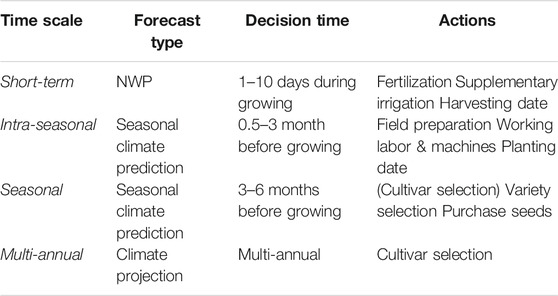
TABLE 1. Farmers tactical decisions and actions across different time scales based on information obtained from RCM simulations, short-term and long-term climate projections and seasonal- and short-term forecasts.
Apart from the direct support of farmers in their tactical decisions, climate information is widely applied in climate change impact studies (CCIS). Together with elevated atmospheric CO2 concentrations and changes in radiation, it is primarily the changes in precipitation and temperature (P and T) that are most crucial for agricultural yield predictions (Pirttioja et al., 2015). Thus, both farmer and CCIS require reliable predictions of P and T.
Regional Climate Models (RCMs) have the potential to provide reliable climate information to support farmers and impact modellers. They are able to provide reliable predictions of P and T, and other climate variables in more general. RCMs are driven by winds, temperature and humidity imposed at the boundaries of the domain, supplied by the General Circulation Models (GCMs), which usually leads to large-scale fields being consistent with the driving GCM (e.g., Maraun et al., 2010).
Long-term RCM projections have been derived in several projects to produce scientific sound and high-resolution climate data, including multi-model ensembles of future climate projections. Such projects are e.g. the Coordinated Regional climate Downscaling Experiment (CORDEX) (Giorgi et al., 2009), including a set of climate projections over Africa (CORDEX-AFRICA, Nikulin et al. (2012)). It is found that many of the CORDEX GCM-RCM combinations significantly improve the representation of P compared to that from their boundary conditions, i.e., the driving GCMs (Nikulin et al., 2012).
It is well-known that the performance of RCM simulations strongly depends on their specific settings, and in particular the physics options. High-resolution RCMs, no matter if they are applied for short-term forecasts or long-term climate projections, need to approximate processes at scales below those that they can resolve. For each physical process, there are numerous alternative parameterization schemes to choose from (Warner, 2010).
Among others, these include processes of radiation (RA), cumulus convection (CU), and cloud microphysics (MP), and planetary boundary layer (PBL), hence requiring parameterization (i.e., model tuning) with different inherent assumptions and approximations. A comprehensive overview is given in Stensrud (2011). The number of adjustable parameters in RCMs is large and typically exceeds 100 (Quan et al., 2016). The computational expenses usually prevent an “optimal” tuning of the single parameters, since the number of model experiments for parameter optimization increases exponentially with parameter dimension, which may result in >104 experiments. For short-term numerical weather prediction (NWP), however, efforts are being made to evaluate the sensitivity of single parameters, and finally to optimize the most influential ones. This is however only possible by means of efficient optimization approaches, computationally low-cost RCM statistical surrogates (model emulators) (Bellprat et al., 2012; Wang et al., 2014), and the help of supercomputers (Quan et al., 2016). Due to required longer simulation periods for evaluating climate simulations, compared to short-term NWP, fine-tuning of single parameters is not possible. In turn, it is the sensitivity of the different parameterization schemes (including predefined parameters) and their interplay, which is in the focus of climate modellers.
Results from parameterization studies for Africa, however, may reveal contradicting conclusions. Endris et al. (2013) analyzed the characteristics of rainfall patterns over East Africa. Their results indicated large sensitivity of WRF model results to the choice of physics parameterizations there. Based on their settings, i.e., Kain Fritsch (KF) CU-, WRF Single-Moment 5-class (WSM5) MP-, Yonsei University (YSU) PBL-, and Dudhia and Rapid Radiative Transfer Model (RRTM) for short- and long wave RA schemes, respectively, they observed wet model biases. In turn, Pohl et al. (2011), concluded that WRF shows the best performance when combining the KF CU scheme, using very similar settings for the other schemes (i.e., WRF Single-Moment 6-class (WSM6) MP-, Asymmetric Convective Model (ACM2) PBL-, Dudhia short wave RA, and the RRTM long wave RA scheme). Recently, Umer et al. (2021) analysed the capacity of WRF in simulation high-intensity rainfall events over the Kampala catchment in Uganda. Using a high-intensity rainfall event that caused a strong local flood hazard, they tested a large variety of parameterization combinations and found that the most successful combination consists of complex microphysics such as the Morrison 2-moment scheme combined with Grell-Freitas (GF) CU- and ACM2 PBL schemes. Otieno et al. (2018) focused their analysis on the performance of four CU schemes (i.e., KF, KF with a moisture-advection based trigger function, Grell Dévényi (GRELL), and Betts Miller Janjic (BMJ) of WRF to simulate mean rainfall patterns, number of rainy days, and vertically integrated moisture flux during a composite of wet years for the Lake Victoria basin in East Africa. They concluded that both, the KF and GRELL schemes showed better performance than the BMJ scheme. Contrasting conclusions were drawn in the study of Argent et al. (2015).
Due to the high complexity of represented processes and partly non-linear interactions between them, weather and climate information is afflicted by high uncertainties which requires a sound selection of combination of the above-mentioned physics schemes. In the best case, a selection is therefore made based on the evaluation of a full factorial set of possible combinations, in combination with a suite of different performance evaluation strategies (Laux et al., 2019).
A large number of different verification scores exists, but not all of them are equally suitable for all variables or objectives. Using traditional point verification scores for quantifying the performance of modeling the spatial patterns of P, error measures such as the mean absolute error (MAE) and root mean squared error (RMSE) may punish RCM simulations twice, i.e., for missing the actual feature in the grid cell, and for predicting it in another grid cell (or region) where no precipitation has occurred. This double-penalty problem (Jolliffe and Stevenson, 2003) motivated the development of object-based approaches (e.g., Wernli et al., 2008; AghaKouchak et al., 2011; Mittermaier, 2014), accounting more specifically for the displacement and spatial structure errors of objects such as precipitation patterns at a given scale. Wernli et al. (2008) proposed the three-component feature-based quality measure SAL, which considers the structure (S), amplitude (A), and location (L) of a precipitation information. SAL has been applied frequently in high-resolution Numerical Weather Prediction (NWP) model development (e.g., Ahijevych et al., 2009; van Weverberg et al., 2010; Wittmann et al., 2010; Zappa et al., 2010; Haiden et al., 2011; Termonia et al., 2011), and -validation (Vincendon et al., 2011; Zimmer et al., 2011; Hardy et al., 2016; Gofa et al., 2018). For its application on ensemble NWP forecasts, an ensemble extension of the structure–amplitude–location (SAL) spatial verification method, called ensemble SAL (eSAL) was introduced (Radanovics et al., 2018).
Recently, another approach to support the identification of optimal configurations of physics parameterizations in RCMs has been developed. This approach makes use of empirical copula functions and considers the representation of the joint dependence structure (covariance structure) between different RCM output variables (Laux et al., 2019). This is particularly important in the field of CCIS such as in agriculture, where the correct representation of the interplay between the different variables (e.g., P and T) needs to be accurately modeled.
This study aims at the identification of a suitable set of physics parameterization combinations in RCM simulations for agricultural decision support in the Northern SSA (NSSA) region. We focus on the validation of P and T, which are considered the most crucial variables in impact models. We follow three different validation strategies, i.e., a traditional domain-based validation (for P and T), an object-based validation (for P only) as well as a station-based validation (for the joint occurrence of P and T), and analyze the RCM performance for a region in NSSA based on 16 parameterization experiments for the period 2006–2010. The experimental setup of the study does not permit to address process-based explanations for differences in the performance of the different physics parameterization combinations. Since the choice of parameterization options depends strongly on the region of interest (i.e., regions within the NSSA domain), the RCM parameterization simulations is being made available to the climate community to facilitate demand-oriented multi-objective validation studies (specific regions across NSSA, specific variables, specific performance scores, etc.).
The data sources used in this study can be grouped into 1) initial and lateral boundary conditions, in order to drive the mesoscale climate model WRF, 2) gridded reference data, and 3) point measurement reference data for model validation.
For this study, the European Centre for Medium-Range Weather Forecasts (ECMWF) ERA-Interim reanalysis is providing “perfect” initial conditions (ICs) and lateral boundary conditions (LBCs) to drive the WRF model. Reanalyses, in general, are suitable data sources since they merge irregular observations and models that encompass most crucial physical and dynamical processes in order to generate a synthesized estimate of the state of the earth system across a uniform grid, with spatial homogeneity, temporal continuity, and a multidimensional hierarchy (Sun et al., 2018).
The ERA-Interim reanalysis system used cycle 31r2 of the Integrated Forecast System (IFS). Data are provided on a reduced Gaussian grid with approximately uniform horizontal 79 km spacing (approximately 0.75°), at 60 vertical levels (with top level at 0.1 hPa). The ICs and LBCs used in WRF are wind components, temperature, water vapor, surface pressure, sea surface temperature (SST) and soil moisture, all of them in different atmospheric and soil height levels, respectively. ERA-Interim is known to be skillful in representing atmospheric processes in different regions worldwide (Lin et al., 2014). It has recently been superseded by the ERA5 reanalysis, which was not available at the beginning of this study. A detailed description of ERA-Interim can be found in Dee et al. (2011).
Different reference data sets are applied for model validation of P and T to analyze the robustness of the findings. The reference data consist of several products:
1) Climate Prediction Center (CPC) Global Temperature dataset has been developed by the American National Oceanic and Atmospheric Administration (NOAA) using the Shepard interpolation algorithm of quality-checked gauge records of the Global Telecommunication System (GTS) network (Fan and van den Dool, 2008). It is available from 1979-01-01 to present in a 0.5° and daily resolution. In order to validate the 16 parameterization runs with the CPC data, the WRF output was additionally upscaled to 0.5° resolution.
2) Climate Hazards Group Infrared Precipitation with Stations (CHIRPS) version 2.0, a blended gauge-satellite precipitation product (Funk et al., 2014). CHIRPS data is a quasi-global (50° S–50° N) dataset with a spatial resolution of 0.05°. It is available from 1981 to near present, as daily, pentadal, and monthly precipitation data. CHIRPS has been developed to support the United States Agency for International Development Famine Early Warning Systems Network (FEWS NET). Building on well-established approaches, CHIRPS applies the Tropical Rainfall Measuring Mission Multi-satellite Precipitation Analysis (TMPA 3B42 v7) to calibrate global Cold Cloud Duration (CCD) rainfall estimates.
3) Multi-Source Weighted-Ensemble Precipitation (MSWEP) version 2.1, a merged precipitation estimates from satellite and reanalysis dataset. MSWEP is a global precipitation product with a 3-hourly and 0.1° resolution available from 1979 to near real-time. The MSWEP dataset merges gauge, satellite and reanalysis data to obtain the highest quality precipitation estimates at every location. MSWEP tends to exhibit better performance in both densely gauged and ungauged regions than other precipitation products (Beck et al., 2017).
4) ERA5-Land climate reanalysis, a reanalysis product of a land component replay of the ECMWF ERA5 reanalysis product (Hersbach et al., 2020; Muñoz-Sabater et al., 2021). ERA5-Land provides hourly data at a horizontal resolution of 0.1° from 1981 to near real-time for land variables at an enhanced resolution (compared to ERA5). Observations are not directly used in the production of ERA5-Land, but have an indirect influence through the applied atmospheric forcing. Atmospheric forcing variables are corrected by a so-called “lapse rate correction” before driving the model, accounting for the altitude difference between the grid of the forcing and the higher resolution grid of ERA5-Land. The temporal and spatial resolutions makes this dataset very useful for applications such as flood or drought forecasting.
Precipitation and temperature data from the Global Historical Climatology Network (GHCN)-Daily is applied to validate the WRF model results at point-scale. GHCN-Daily contains records from over 100,000 stations in 180 countries and originates from a variety of sources ranging from paper forms completed by volunteer observers to synoptic reports from automated weather stations, some of which date back to the mid-1800s. It is maintained and quality checked by the National Oceanic and Atmospheric Administration’s (NOAA) National Climatic Data Center (NCDC) (Durre et al., 2010). The data has proven useful in many applications requiring daily data (e.g., Alexander et al., 2006).
It is well-known that the hydro-meteorological station network across NSSA is sparse in general (Caesar et al., 2006) and time series usually contain a lot of missing values (MVs), in particular for data on daily resolution. Stations have been manually pre-selected by visual inspection of data availability during the period of interest (2006–2010).
Based on the overall availability, the length of data gaps, and further subjective decisions (e.g., distribution of data gaps within the year) during 2006–2010, 79 stations for daily precipitation amount and 64 stations for daily mean temperature have been pre-selected and applied for validation (Figure 1). Altogether, 52 stations having both variables (i.e., the P and T pairs) are available, which are applied in the subsequent evaluation. Even though the overall amount of missing values (MVs) can reach about 90% for some of the stations, they have been selected because they contain a significant (>10% has been considered as significant for this data sparse region) amount of continuous data during this period.
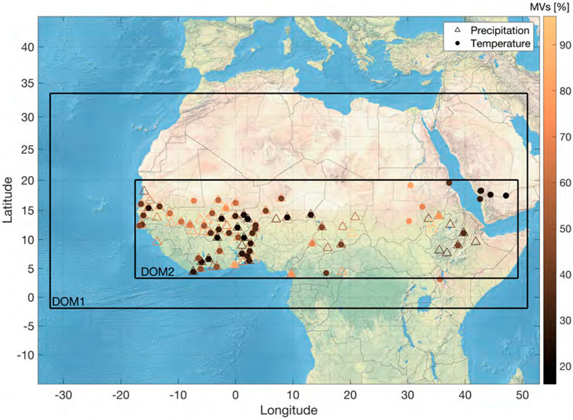
FIGURE 1. Domain configuration for the WRF simulations. See Table 2 for further information about the horizontal resolutions for the different nests, respectively. Availability of observations stations from the Global Historical Climatology Network-Daily (GHCN-D) database. The color of the dots indicates the number of missing values (MVs, in %) for the period 2006–2010.
The description of 1) the general WRF setup is followed by 2) the applied 16-member physics ensemble, and 3) the different applied validation strategies.
In this study, the mesoscale Weather Research and Forecasting Model (WRF, Version v3.9) is applied following a one-way nesting approach with two domains (Figure 1), driven by ERA-Interim initial conditions (ICs) and lateral boundary conditions (LBCs).
During the model integration, the meteorological LBCs are updated every 6 h, i.e., at 00:00, 06:00, 12:00, and 18:00 UTC, respectively. The model integration time was set to 90s for domain 1, with a parent-to-nest time step ratio of 1:3, i.e., 30 s for domain 2 (Table 2).
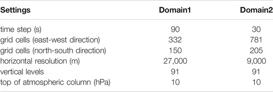
TABLE 2. WRF domain settings applied in the parameterization experiments.
The SST has been updated every 6 h, as provided by the ERA-Interim data. The ERA5 reanalysis also provide time-dependent sea surface temperatures (SSTs) and soil moisture content in different levels below surface as input for the WRF. Over land, different other land surface characteristics are obtained from the NOAH-LSM. In this study, a 3-month period (October 1st—December 31st, 2005) has been simulated to spin-up the model runs. This time, which is expected to be sufficient for the WRF model to build up the relevant atmospheric circulation features, has not been considered for the analyses.
Testing of all available physics schemes of WRF is a computationally very expensive task. Considering the trade-offs between computational expenses and the requirements on a sufficiently long simulation period required for a robust validation, we decided to apply a set of 16 WRF parameterization combinations for five consecutive years from 2006–2010 (Table 3). This period has been selected as it contains relatively wet as well as dry years, corresponding to different ENSO states. It is also worth to mention that the impact of ENSO varies across the region (e.g., Gizaw and Gan, 2017). This 16-member-physics ensemble consists of two cumulus (CU) schemes, two microphysics (MP) schemes, two planetary boundary layer (PBL) schemes, and two radiation (RA) schemes.
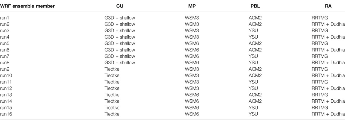
TABLE 3. Full factorial WRF parameterization combinations, consisting of two cumulus parameterization (CU), two microphysic parameterization (MP), two planatery boundary layer parameterization (PBL), and two radiation parameterization (RA) schemes.
The WRF model represents the following different physical processes: microphysics, cumulus convection, near-surface physics, land-surface physics, planetary boundary layer physics, and atmospheric radiative (long-wave and short-wave) transfer. A brief overview of the tested schemes is given in the following: A CU parameterization, in general, determines the effects of sub-grid-scale convection on the modeled atmosphere. More precisely, resolved-scale variables are used by the CU scheme to diagnose whether or not convection exists, and if so, to determine its impacts on resolved-scale variables. In this study, we test the two different mass-flux type schemes of G3D (improved Grell-Dévényi scheme, Grell and Dévényi (2002)) and the New Tiedtke scheme (Tiedtke, 1989; Zhang and Wang, 2017), which consider updrafts explicitly, i.e. transport air from the updraft source layer upwards while reducing the convective available potential energy (CAPE). For G3D, an additional option for shallow convection is applied. This scheme represents non-precipitating (except for drizzle precipitation) shallow clouds by enhanced mass-flux.
Besides the CU parameterizations, which are needed for modeling at grid resolutions exceeding about 4 km (Prein et al., 2015), there will always exist the need to parameterize MP schemes due to the processes involved, which exist on scales of hydrometeors, ranging from molecular to micrometer scales. The representation of these processes determines the skill with which type, amount, and spatial distribution of precipitation can be simulated. MP are also important in long-term climate projections, since the atmosphere may respond to increases in greenhouse gases with an alteration in (global) cloud properties as well as albedo. This, in turn, may have consequences on global warming by positive or negative feedbacks. Moreover, microphysical impacts of increased aerosols in the atmosphere of a changed climate can change precipitation efficiency (Warner, 2010). In this study, we applied the WRF single moment 3-class simple ice scheme (WSM3, Hong et al. (2004)) as well as the more complex WRF single-moment 6-class (WSM6, Hong et al. (2006)) scheme. WSM6 represents in addition to simulated mixing ratios for water vapor, cloud ice crystals, snow, water vapor, cloud liquid water, rain liquid water, also graupel. Both WSM3 and WSM6, do not represent hail.
The planetary boundary layer (PBL) scheme parameterizes the processes of the atmosphere near the surface where the influence of the surface is determined through turbulent exchange of momentum, heat, and moisture. Since these processes occur on a sub-grid scale, they need to be parameterized. The zone in between the surface and the free atmosphere is characterized by vertical diffusion due to turbulent motion. The PBL height may vary between approximately 100 m during night (over land) up to a few thousand metres during daytime with strong surface heating. In conjunction with the surface parameterization, the PBL schemes determines the surface fluxes within the boundary layer. In this study the Yonsei University (YSU, Hong et al. (2006)) and the Asymmetrical Convective Model version 2 (ACM2, Pleim (2007)) are applied, which both generally allow for turbulent mixing with distant, i.e., nonlocal, grid cells. While YSU explicitly determines the entrainment layer at the top of the PBL based on large-eddy simulations, ACM2 combines explicit nonlocal exchange from the surface to all layers above subsequently by local eddy diffusion.
Processes such as the absorption by the atmosphere, clouds, and dust, scattering by air molecules and dust, and reflection by clouds and dust are typically represented by radiation parameterization schemes. In this study, we applied two different combinations of radiation schemes, i.e. the Rapid Radiative Transfer Model (RRTM, Clough et al. (2005)) and Dudhia scheme (Dudhia, 1989) and the Rapid Radiative Transfer Model for GCMs (RRTMG, Iacono et al. (2008)) scheme for both long-wave (LW) and shortwave (SW), respectively. RRTMG is computationally more expensive, considering subgrid-scale cloud variability using a statistical approach of maximum-random cloud overlap, whereas RRTM + Dudhia applies an approach of binary cloud fraction only.
Traditional statistical performance scores such as the Pearson correlation coefficient (r), the standard deviation (SD), the root-mean-square error (RMSE) as well as the density function are calculated. These three scores are summarized as Taylor diagrams (Taylor, 2001), which facilitates a comparative assessment of the different parameterization runs. In order to avoid the dry season in NSSA to artificially improve the model performance, we considered only the core rainy season (June–August, JJA), a period with significant rainfall across NSSA in domain 2. The validation in this study is performed for the average of domain 2.
Apart from domain-based approaches, object-based approaches can consider the displacement and the spatial structure errors at a given scale. In this study, the three-component feature-based quality measure SAL approach Wernli et al. (2008) as well as the ensemble extension of SAL (eSAL) (Radanovics et al., 2018) are followed, which consider the structure (S), the amplitude (A), and the location (L) of a quantitative precipitation forecast, as e.g. obtained by RCMs. More technical details about the eSAL algorithms can be found in the Supplementary Material S1 (Methodologies, section 1.1).
The analysis is carried out for each parameterization class individually. Therefore, ensembles are generated for the different schemes in a first step to obtain more robust conclusions for the different schemes. For the CU schemes, runs #1–8 representing the G3D scheme are jointly analyzed and compared to runs #9–16. Likewise, the ensemble generation is repeated for the MP, the PBL, and the RA schemes, each of these parameterization classes containing two different schemes with eight representing runs to be compared.
In addition to the domain-based validation, separately conducted for P and T and object-based validation (conducted for P only), we followed the selection approach developed by Laux et al. (2019), which considers the joint dependence structure (i.e., the covariance structure) between P and T. The selection is based on empirical P and T copula functions and the χ2-test. The concept of copulas has been extensively used in various fields of hydrology and meteorology, such as for improving the spatial resolution of modeled precipitation (Van Den Berg et al., 2011), for bias-correcting the output from RCMs (e.g. Laux et al., 2011; Mao et al., 2015), and for data fusion (Vogl et al., 2012; Lorenz et al., 2018).
The statistical relationship between P and T is described by an empirical copula function, which is according to Genest et al. (2009) the most objective approximation of the underlying dependence structure. The empirical copula function can be understood as the bivariate density in the rank space of the data. We compared the observed empirical copula function to the simulated P and T copulas of the 16 RCM physics parameterization simulations. We thereby relied on raw observation station data exclusively since the results of this approach are suspected to be very prone to interpolation errors, especially in data sparse regions such as NSSA. Gridded interpolated data sets might fail to capture the true underlying dependence structure.
From the 16 different conducted WRF parameterization runs (see Table 2), we extracted the modeled P and T tuples from the corresponding RCM grid cells, which contain both P and T observation data (Figure 1). Practically, only the positive P and T pairs (i.e., pairs in which p > 0) are considered. More technical details are found in the Supplementary Material S1 (Methodologies, section 1.2).
In order to quantify the relative impact of the CU-, MP-, PBL-, and RA scheme, the dispersion of the simulated distributions is analysed in a first step. For this reason, subgroup-ensembles for each scheme are generated. For the CU scheme, for instance, the G3D and the Tiedtke ensembles are generated, each of them consisting of eight members. G3D consists of run #1–8, Tiedtke consists of run #9–16 (see Table 3). The same procedure is repeated for the subgroup-ensembles of the MP-, the PBL-, and the RA scheme.
It can be seen from Figure 2 that the relative differences of the simulated distributions for P between the subgroups are relatively high for the applied CU- and the RA schemes, i.e., between G3D and Tiedtke, as well as between RRTMG and RRTM + Dudhia. For the applied MP- and PBL schemes, the simulated subgroup distributions are similar. This indicates the relative importance of the different schemes on the dispersion of the simulated distribution. This impact is higher for P than for T (not shown).
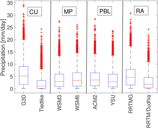
FIGURE 2. Simulated subgroup-ensemble distributions of mean daily precipitation values for the period 2006–2010. Each box-whisker plot represents the distribution within the NSSA domain for each subgroup-ensemble. Each subgroup-ensemble consists of eight ensemble members.
In the next step, the simulated data will be validated against reference data. Figure 3 illustrates Taylor diagrams using the ERA5-Land climate reanalysis data as reference for P (left) and T (right). It can be seen that for P, high correlation coefficients of around 0.85 can be obtained. Normalized standard deviations range between 0.75 and about 1.75 and are thus in an acceptable range of the reference data, and RMSE values range between approx. 0.25 and 1 mm/d, depending on the parameterization setting. In general, it can be seen the G3D convection scheme performs better than the Tiedtke scheme. The runs #2 and #3, however, show a reduced performance compared to the other 6 G3D convection runs (i.e., run #1 and runs #4–8). Very similar patterns, however with reduced correlation coefficients and increased standard deviations and RMSE values, are found using the other two P reference data sets MSWEP and CHIRPS (see Supplementary Figure S1). The performance of the simulated T is very high for most of the 16 runs. The correlation coefficients mostly exceed 0.85 and normalized standard deviations are found to be too low compared to the reference data. Most of the RMSE values lie within 0.25 and 0.5 mm/d. Exceptions are runs #12 and #15, with correlation coefficients slightly exceeding 0.3, normalized standard deviations of around 0.25, and RMSE values of about 0.75°C. Overall, the dispersion between the T runs within the Taylor plot is comparatively smaller than that for the P runs. Again, similar results are obtained for the second T reference data set CPC (see Supplementary Figure S2). The classical domain-based validation based on the Taylor diagrams gives clear indication that the G3D convection runs are superior over the Tiedtke convection scheme. This can be clearly seen for P, but this is much less pronounced for T.
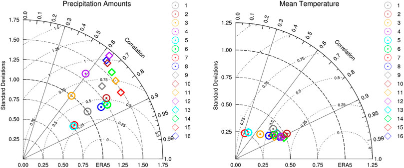
FIGURE 3. Taylor diagrams, depicting the Pearson correlation coefficient (straight lines), the normalized standard deviation (dashed lines) and the root-mean-square error (RMSE) (dotted lines) between simulated JJA precipitation amounts (left) and JJA mean temperature (right) of the 16 ensemble members and ERA5-Land reanalysis as reference data for the period 2006–2010.
Apart from the Taylor diagrams, the probability density function (PDF) gives additional valuable information concerning the distribution of the P and T values in the NSSA domain. The PDF does however not consider the temporal evolution of the variables. Figure 4 (left) illustrates the PDF of the G3D cumulus runs, while Figure 4 (right) depicts the Tiedtke runs. Despite of the good results of G3D obtained by the Taylor diagram evaluation, it is found that most of the G3D runs highly overestimate daily rainfall values compared to the reference data. Large discrepancies are found for these runs, with the peak of the PDF ranging from approximately 6 mm/d (run #4) to 14 mm/d (runs #1 and #5). In general, the modeled G3D distributions are wider and do not show a bimodal shape as can be observed in the CHIRPS and ERA5-Land reference data. In turn, the Tiedtke runs show more realistic distributions concerning their shapes but also their peak values. Based on the assessment of the PDF, runs #10, 12, 14, and 16 can represent quite well the PDFs of the reference data, runs #9, 11, 13, and 15 show a slightly widened distribution with reduced peak probability values. Moreover, the latter runs are shifted to the right, i.e., lead to wet biases.
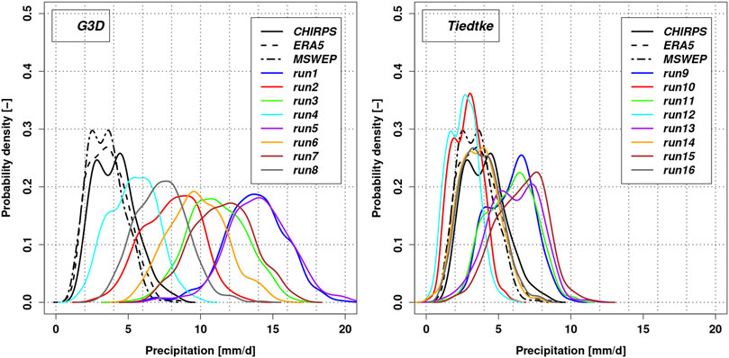
FIGURE 4. Probability Density Function (PDF) of simulated (JJA) daily mean precipitation in the WRF runs using G3D(left) and Tiedtke convection scheme (right) for domain 2 (2006–2010). CHIRPS, ERA5-Land, and MSWEP are given as reference precipitation.
For temperature, all of the 16 parameterization runs show a remarkable cold bias compared to the reference data sets (CPC and ERA5-Land) (Figure 5). While the bias is on average approximately 1°K larger for the G3D run.
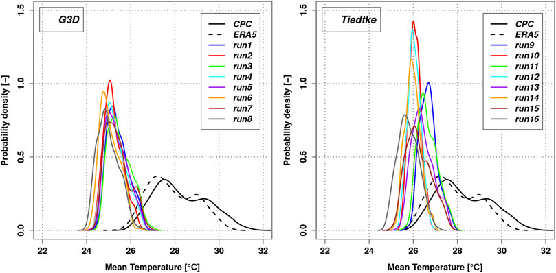
FIGURE 5. Probability Density Function (PDF) of the simulated (JJA) daily mean temperature in the 16 WRF runs using G3D(left) and Tiedtke convection scheme (right) for domain 2 (2006–2010). CPC and ERA5-Land are given as reference precipitation.
Figure 6 illustrates the validation of domain-averaged precipitation in terms of the amplitude (A), the structure or volume (S), and the location (L) of precipitation objects for the ensemble runs (abbreviated by e, i.e., eA, eS, eL, respectively) (Radanovics et al., 2018) representing the CU- (i.e., G3D and Tiedtke, given in blue), the RA- (i.e., RRTMG and RRTM, given in orange), the MP- (i.e., WSM3 and WSM6, given in grey), and the PBL (i.e., YSU and ACM2, given in magenta) schemes. The reference domain average precipitation (MeanP, in the 4th row of each plot) is used to relate the errors of eA, eS, and eL to the ERA5-Land data of the same period (2006–2010). The main diagonal represents the histograms of eA, eS, and eL of the respective physics ensemble and of MeanP.
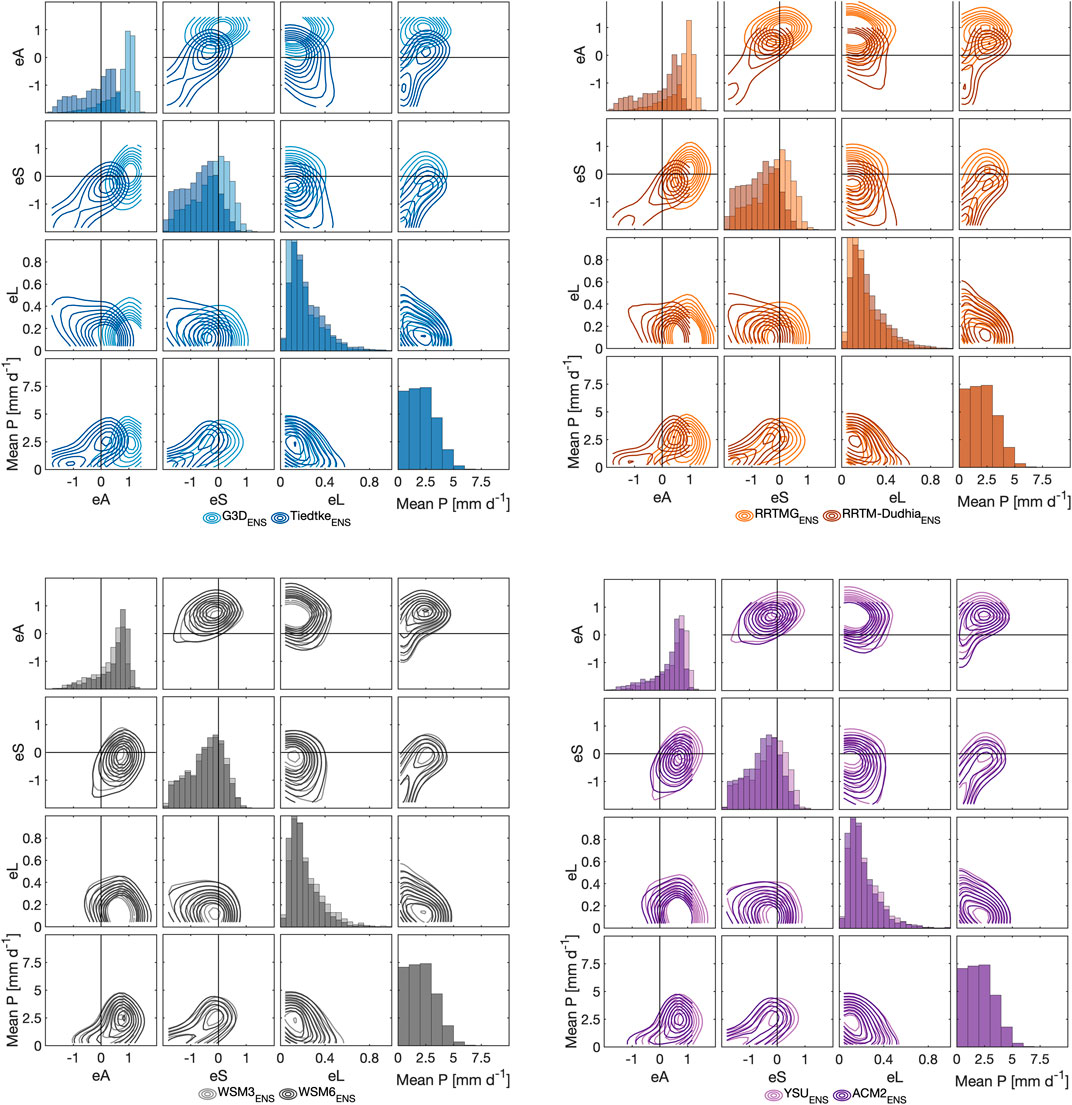
FIGURE 6. Validation of the domain-averaged precipitation (amplitude, A), the structure (volume, S), and the location (L) of precipitation objects for the ensembles (e), consisting of eight cumulus- (blue), radiation- (orange), microphysics- (grey), and planetary boundary layer (magenta) parameterization runs, respectively (see Table 2), for the period 2006–2010. The reference data is the ERA5-Land. Note that all the subplots are symmetrical to the main diagonal.
In general, it can be seen that the differences between G3D and Tiedtke ensembles (blue) and between RRTMG and RRTM-Dudhia ensembles (orange) are relatively large compared to the differences between WSM3 and WSM6 (grey) and between YSU and ACM2 (magenta). This highlights the general importance of the CU- as well as the RA parameterization for the representation of P in RCMs. For this reason, mainly the CU- and RA parameterization ensembles are contrasted in terms of an object-based validation in the following description of the results.
With respect to the CU ensembles, it can be seen that mainly the G3D ensemble overestimate the domain-averaged precipitation (eA > 0). At the same time, the structure (eS around zero) is well captured. The G3D ensemble shows predominantly a positive amplitude errors (eA), whereas Tiedtke shows both positive and negative eA. This means that the G3D ensemble is characterized by a clear wet bias and the Tiedtke runs may have a wet or a dry bias. This confirms the results obtained from the domain-based validation (see Figure 4). The positive eA of G3D is found particularly for medium reference domain-averaged precipitation (MeanP) between 2 and 3 mm/d. Moreover, G3D exhibits both positive and negative structure error (eS), a negative eS for small (<2 mm/d) reference domain-averaged precipitation values, and a tendency of smaller location errors (eL) compared to the Tiedtke ensemble. In turn, Tiedtke is characterized by small positive eA and small negative eS for the reference precipitation between 2 and 3 mm/d, but also by negative eA for reference precipitation values <2 mm/d. In addition, the Tiedtke ensemble shows large negative eS (too small or too peaked), and slightly increased eL for small reference precipitation values compared to the G3D ensemble.
Similar findings are obtained for the reference data sets of MSWEP and CHIRPS (Supplementary Figures S3, S4).
In addition to the domain-based validation, both separately conducted for P and T and object-based validation (conducted for P only), we follow another approach, which considers the joint dependence structure between P and T by using station data for evaluation. Based on all available observation station data across NSSA (see their distribution in Figure 1), the composite empirical Copula for the entire region is calculated (Figure 7). It shows the pure P and T dependency structure in the rank space of the data across entire NSSA. Enhanced densities are found for low rainfall rates and high temperatures as well as for high rainfall rates and low temperature values. The density is also enhanced in the central quantile ranges of both variables, thus the empirical Copula describes a typical elliptic shape with enhanced densities at the secondary diagonal. The density is reduced in the lower left and the upper right quadrant of the graph.
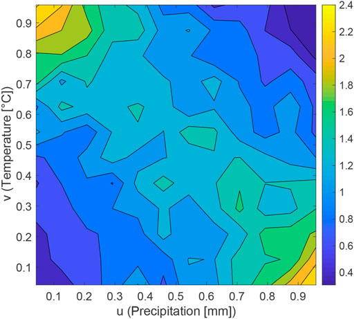
FIGURE 7. Composite empirical copula with joint P and T pairs from all stations of GHCN-D data during the period 2006–2010. See Figure 1 for observation stations included in the calculation.
Comparing the shape of the observed joint dependency function of P and T with the modeled dependency function of the 16 parameterization runs may give additional indication of the fidelity of RCM simulations in reproducing the observed regional climate (Figure 8). Apart from runs #10, 13, and 14, the elliptic shape can be generally confirmed for all other runs. As the density is a proxy for the level of dependency between two variables, we have calculated the χ2-test statistics to decide quantitatively on the parameterization scheme to be selected.
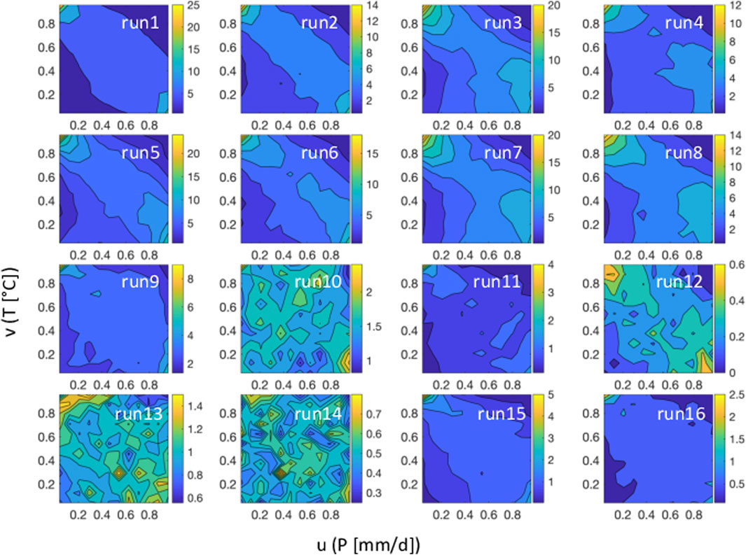
FIGURE 8. Empirical Copula with joint P and T pairs from the 16 WRF simulations at locations from the included P and T pairs from GHCN-D data during the period 2006–2010. See Figure 1 for observation stations included in this analysis. Note that the Copula densities have different scaling for better visibility of the density shapes.
Table 4 displays the minimum p-values for which the h0 hypothesis (i.e., the modeled P and T data come from the same distribution as the observed data) can be rejected. Small values close to zero cast doubt on independence. In this case one would rather accept the h1 hypothesis (i.e., the modeled and observed P and T data come from different distributions). Based on the retained p-values of the χ2-test (Table 4), one would rather select the Tiedtke than the G3D parameterization runs, with exception of the runs #10 and 14. This is almost consistent with the expectations based on the visual interpretation of Figure 8.
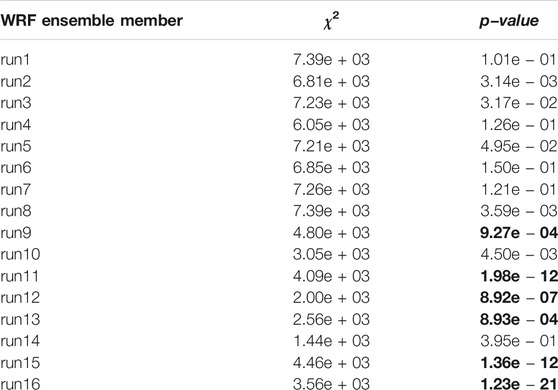
TABLE 4. χ2-values and p-values of the χ2-tests for the 16 parameterization runs (2006–2010). Values < 1.0e−03 are bolded.
The RCM skill related to physics parameterizations depends on a multitude of factors such as the target region, the variables of interest. Since optimizing all single physics parameters is computationally very demanding (e.g., Bellprat et al., 2012; Wang et al., 2014; Quan et al., 2016), and thus virtually not possible for climate simulations, this study targets at the evaluation of different physics parameterization schemes.
We followed a full factorial experimental framework, containing two schemes for CU, MP, RA, and PBL, respectively, leading to 24 runs. A full factorial setup is required to analyse possible interactions between the different parameterization schemes (Warner, 2010). High computational costs of RCM simulations limit the number of schemes as well as the simulation period to be analyzed. So far, little effort has been devoted to physics ensemble experiments using multiple years as simulation period, although long periods would be preferential for obtaining more reliable climate simulation (Argüeso et al., 2011). Thus, for the experimental design there is always a trade-off between the length of the simulation period and the number of tested physics parameterization schemes. This is confirmed by Portele et al. (2021), who applied two more CU schemes in their study, resulting in a setup consisting of 32 experiments.
We applied domain-based approaches using well-established Taylor diagrams in combination with the PDF for P and T. From the results obtained, it becomes obvious that global validation scores such as the Pearson correlation coefficient or the RMSE (provided by the Taylor diagram) might not urgently be the best choice alone to quantify the skill of the RCM simulation results, and thus meet a decision on the optimal parameterization scheme. For P, for instance, it turned out that suitable candidates based on the G3D CU scheme is partly afflicted with wet biases, which becomes obvious when looking at the PDFs of the simulations. However, the PDF alone ignores the temporal evolution of the variables and is thus not suitable if considered as the only approach for candidate selection. The results obtained indicate that there exist strong interactions between the CU scheme and the other schemes, leading to a relatively high dispersion of the data points for P in the Taylor diagram and relatively large discrepancies in the PDFs. The impact of the interactions seems to be larger for the G3D scheme that for Tiedtke scheme. Moreover, all the applied experiments led to cold biases. This indicates that the RCM simulations based on these settings cannot be applied to impact assessment studies without reservation. In process-based impact models (e.g., crop models), where non-linear processes such as heat stress are considered, such cold biases would need corrections (e.g., Siegmund et al., 2015; Laux et al., 2021) before in order to obtain reliable yield predictions.
Moreover, we applied an object-based approach from NWP for the evaluation, which considers the displacement and spatial structure error of P (Radanovics et al., 2018). The results confirmed the findings of higher dispersion from the CU schemes compared to other schemes of RA, MP, and PBL, obtained by the domain-based evaluation. Similar findings for the object-based approach are reported in Portele et al. (2021).
In addition, we applied a station-based validation strategy based on the concept of the empirical Copula to analyze the representation of the covariance between P and T (Laux et al., 2019). This strategy confirmed the better performance of the Tiedtke schemes compared to the G3D scheme. It is obvious that the representation of extremes is overestimated in all combinations with G3D schemes, as can be seen from the increased densities, partly by a factor of 10.
While the object-based approach might be more useful in NWP to predict e.g. the exact location of thunderstorms and patterns of P, the grid- and station-based evaluation approaches might be more crucial for climate impact assessment studies. In impact models (e.g., agricultural or hydrological models), in which the physiological processes are described using of non-linear response or threshold-based equations, the correct representation of crop-relevant variables and their interplay (between P and T, but also between other variables such as radiation, wind speed, relative humidity) is of utmost importance. Biases of the single variables but also distortions in their joint occurrence may negatively affect the results in CCIS. In contrast to other parameterization studies (e.g., Portele et al., 2021; Yang et al., 2021), relatively long simulation periods (here at least five years) are necessary to follow this station-based approach. T and P tuples with sufficient non-zero values of P are required for a robust calculation of the joint T and P dependency structure. The intermittency of P (Trenberth et al., 2017) is increasing the length of the RCM simulation period for this kind of evaluation. This is particularly problematic in arid- or semi-arid regions as prevail in large parts across NSSA, where the rainy is limited to a few months only. A sparse observation network and data gaps in NSSA (e.g., van de Giesen et al., 2014) further complicate this kind of evaluation.
While the grid-based approach is usually related with traditional point verification scores, the station- and the object-based approach use other non-traditional evaluation scores. The selection of evaluation scores always depends on the objectives. For agricultural impact assessment, for instance, the correct representation of dry and wet spell probabilities might be more important than the overall precipitation amounts (e.g., Hansen et al., 2006; Mupangwa et al., 2011). Tailor-made validation scores addressing these parameters would have tremendous potential to improve climate simulations at the end.
The study is limited in the following aspects:
• For T, most of the applied parameterization experiments exhibit high correlations with the reference data sets, while the magnitude of the biases remain relatively high. The effects of other parameterization schemes related to RA, and in particular to the shortwave (SW) incoming radiation will be subject of future research.
• A thorough evaluation requires reliable observations. For NSSA, the density of the observation network can be characterized as sparse. This not only affects the quality of the evaluation based on observation stations, but also affects quality of other evaluation strategies using interpolated and merged data sets. The new Trans-African Hydro-Meteorological Observatory (TAHMO) initiative to increase the observation station density in Africa (van de Giesen et al., 2014) might help to facilitate more robust model validation in the future. Since TAHMO relies on cost-effective sensors and transmission technologies, quality assessment studies are necessary prior to their use in model validation studies.
• For the evaluation of the RCM simulations, it is focused on two surface variables only (P and T). Observation data of other variables are only rarely available for NSSA, and including additional variables would further restrict the number of stations with joint data coverage for the station-based validation. It is worth to stress that the actual underlying dependency structure can be reliably derived only from raw observations (i.e., data from point observations). Particularly in data-sparse regions, the Copula-based approach cannot be applied using gridded observations due to the high interpolation uncertainties resulting from the sparse network density.
• Moreover, the spatial distribution of the resulting bias structures from the different parameterization experiments is not analyzed in this study, and in combination to that, the skill of the WRF model to simulate the main governing monsoonal processes in the upper atmosphere such as location and magnitude of African Easterly Waves (AEWs) and the Tropical Easterly Jet (TEJ) (Klein et al., 2015).
• Although supported by the results from Portele et al. (2021), there remain uncertainties related to the sensitivities of the different schemes due to the limited number of two parameterization options for the CU-, MP-, PBL-, and RA scheme, respectively. The results from including more than two options could potentially lead to different conclusions.
• Not all available parameterization schemes could be analyzed due to computational constraints in this study. Glotfelty et al. (2021) reported about some limitation of the WRF-default land surface model, i.e., the Noah-LSM (applied in this study), which does not represent crucial surface parameters such as surface albedo, leaf area index, and surface roughness with sufficient accuracy in some regions over Sub-Saharan Africa. In order to analyze and screen out statistically significant schemes and their interactions, Song et al. (2020) suggested a factorial sensitivity analysis method based on RegCM4 simulations with affordable computational costs. Since the full factorial design might be computationally too expensive for the WRF model, the authors suggest to modify the current framework through integrating fractional factorial method.
• A skill comparison and analysis of potential added-value of the higher resolution compared to the CORDEX-Africa simulations would be an interesting study to come. Of particular interest is the skill in the representation of the diurnal cycle of P, which is known to be out of phase for the majority of the CORDEX RCMs (Nikulin et al., 2012).
We derived an ensemble of 16 WRF physics parameterization experiments and evaluated their performance for NSSA in the period 2006–2010. We used two different CU-, MP-, PBL-, and RA schemes, respectively. We applied traditional (Taylor diagram, probability densities) and more innovative validation metrics (eSAL, Copula functions) for their validation against different P and T observation data. With the specific experimental setup, we found that the selection of the CU parameterization scheme has resulted in the highest impact with respect to the representation of P, followed by the RA parameterization scheme. The G3D CU scheme, in general, let to partly high model overestimation (wet biases) of P and stronger model underestimation (cold biases) of T compared to the Tiedtke scheme. Both, the PBL as well as the MP scheme showed much less impact on the WRF model results. Due to the limited number of parameterization schemes for CU, MP, PBL, and RA, respectively, general conclusions about the sensitivity of the parameterization schemes remain uncertain. The Tiedtke scheme could better represent the observed covariance structure of P and T across NSSA. All parameterization schemes showed relatively high cold biases and too narrow and too peaky modeled PDFs. Overall, we observed an agreement in the assessment based on the different evaluation strategies. However, some features only became obvious when looking at different aspects such as the Taylor diagrams in combination with the PDFs in the domain-based evaluation approach. As all of the applied evaluation approaches have their specific strengths and weaknesses, we suggest to follow a multi-facet evaluation based on different approaches as well as evaluation scores. The specific conclusions about suitable physical parameterization schemes may not hold true for other regions, they may even vary within the study area considered in this study. We therefore want to stimulate the development of further evaluation scores, tailed to the specific objectives of the weather and climate simulations or subsequent impact studies over specific (sub-)regions in NSSA. For this reason, 15 selected climate variables, typically used in agricultural and hydrological climate impact models of the generated physics ensemble are provided as a test bed to facilitate own evaluation studies (see DATA AVAILABILITY STATEMENT below). Yet another crucial unanswered question is whether or not the findings from the reanalysis-based WRF evaluation can be transferred to other forecasts, i.e., short-term NWP or (sub)seasonal forecasts driven by different initial and boundary conditions. The overall conclusions from this study might not only be relevant for the WRF community, but for the broader RCM community.
Publicly available datasets were analyzed in this study. This data can be found here: https://www.ncdc.noaa.gov/, ftp://ftp.cpc.ncep.noaa.gov/precip/PEOPLE/wd52ws/global_temp/, https://data.chc.ucsb.edu/products/CHIRPS-2.0/, http://www.gloh2o.org/, https://doi.org/10.24381/cds.e2161bac.
PL conceptualized this study. PL performed the model simulations and conceived the analysis, supported by DD and TP. PL drafted the first version of the manuscript and processed the data for archiving. All authors discussed and reviewed the manuscript.
The authors declare that the research was conducted in the absence of any commercial or financial relationships that could be construed as a potential conflict of interest.
All claims expressed in this article are solely those of the authors and do not necessarily represent those of their affiliated organizations, or those of the publisher, the editors and the reviewers. Any product that may be evaluated in this article, or claim that may be made by its manufacturer, is not guaranteed or endorsed by the publisher.
The WRF parameterization runs were performed on the supercomputer ForHLR at Steinbuch Centre for Computing (SCC) at KIT, funded by the Ministry of Science, Research and the Arts Baden-Württemberg and by the German Federal Ministry of Education and Research (BMBF). We acknowledge the support from German Climate Computing Center (DKRZ) for archiving the parameterization data sets. Special thanks to Hartmut Häfner (SCC) and Heinke Höck (DKRZ) for their support. We acknowledge financial support from the German Federal Ministry of Education and Research (BMBF) within the project Seasonal Water Resources Management: Regionalized Global Data and Transfer to Practice (SaWaM, grant number 02WGR1421), the German Research Foundation (DFG) through the FOR 2936: Climate Change and Health in Sub-Saharan Africa project (grant number KU2090/14-1), and the African Union (AU) through the Upscaling climate-smart agriculture and land use practices to enhance production systems in West-Africa (UPSCALERS) project (grant number AURG II-1-074-2016).
The Supplementary Material for this article can be found online at: https://www.frontiersin.org/articles/10.3389/feart.2021.700249/full#supplementary-material
AghaKouchak, A., Behrangi, A., Sorooshian, S., Hsu, K., and Amitai, E. (2011). Evaluation of Satellite-Retrieved Extreme Precipitation Rates across the Central United States. J. Geophys. Res. 116, D02115. doi:10.1029/2010JD014741
Ahijevych, D., Gilleland, E., Brown, B. G., and Ebert, E. E. (2009). Application of Spatial Verification Methods to Idealized and NWP-Gridded Precipitation Forecasts. Weather Forecast. 24, 1485–1497. doi:10.1175/2009WAF2222298.1
Alexander, L. V., Zhang, X., Peterson, T. C., Caesar, J., Gleason, B., Tank, A. M. G. K., et al. (2006). Global Observed Changes in Daily Climate Extremes of Temperature and Precipitation. J. Geophys. Res. 111, 1–22. doi:10.1029/2005jd006290
Argent, R., Sun, X., Semazzi, F., Xie, L., and Liu, B. (2015). The Development of a Customization Framework for the WRF Model over the lake Victoria basin, Eastern Africa on Seasonal Timescales. Adv. Meteorology. 2015, 1–15. doi:10.1155/2015/653473
Argüeso, D., Hidalgo-Muñoz, J. M., Gámiz-Fortis, S. R., Esteban-Parra, M. J., Dudhia, J., and Castro-Díez, Y. (2011). Evaluation of WRF Parameterizations for Climate Studies over Southern Spain Using a Multistep Regionalization. J. Clim. 24, 5633–5651. doi:10.1175/JCLI-D-11-00073.1
Beck, H. E., Van Dijk, A. I., Levizzani, V., Schellekens, J., Miralles, D. G., Martens, B., et al. (2017). MSWEP: 3-hourly 0.25° Global Gridded Precipitation (1979-2015) by Merging Gauge, Satellite, and Reanalysis Data. Hydrol. Earth Syst. Sci. 21, 589–615. doi:10.5194/hess-21-589-2017
Bellprat, O., Kotlarski, S., Lüthi, D., and Schär, C. (2012). Objective Calibration of Regional Climate Models. J. Geophys. Res. 117, D23115. doi:10.1029/2012JD018262
Caesar, J., Alexander, L., and Vose, R. (2006). Large-scale Changes in Observed Daily Maximum and Minimum Temperatures: Creation and Analysis of a New Gridded Data Set. J. Geophys. Res. 111, 1–10. doi:10.1029/2005JD006280
Clough, S. A., Shephard, M. W., Mlawer, E. J., Delamere, J. S., Iacono, M. J., Cady-Pereira, K., et al. (2005). Atmospheric Radiative Transfer Modeling: A Summary of the AER Codes. J. Quantitative Spectrosc. Radiative Transfer. 91, 233–244. doi:10.1016/j.jqsrt.2004.05.058
Dee, D. P., Uppala, S. M., Simmons, A. J., Berrisford, P., Poli, P., Kobayashi, S., et al. (2011). The ERA-Interim Reanalysis: Configuration and Performance of the Data Assimilation System. Q.J.R. Meteorol. Soc. 137, 553–597. doi:10.1002/qj.828
Dudhia, J. (1989). Numerical Study of Convection Observed during the Winter Monsoon Experiment Using a Mesoscale Two-Dimensional Model. J. Atmos. Sci. 46, 3077–3107. doi:10.1175/1520-0469(1989)046<3077:nsocod>2.0.co;2
Durre, I., Menne, M. J., Gleason, B. E., Houston, T. G., and Vose, R. S. (2010). Comprehensive Automated Quality Assurance of Daily Surface Observations. J. Appl. Meteorology Climatology. 49, 1615–1633. doi:10.1175/2010JAMC2375.1
Endris, H. S., Omondi, P., Jain, S., Lennard, C., Hewitson, B., Chang'a, L., et al. (2013). Assessment of the Performance of CORDEX Regional Climate Models in Simulating East African Rainfall. J. Clim. 26, 8453–8475. doi:10.1175/jcli-d-12-00708.1
Fan, Y., and van den Dool, H. (2008). A Global Monthly Land Surface Air Temperature Analysis for 1948-present. J. Geophys. Res. 113, 1–18. doi:10.1029/2007JD008470
Funk, C. C., Peterson, P. J., Landsfeld, M. F., Pedreros, D. H., Verdin, J. P., Rowland, J. D., et al. (2014). A Quasi-Global Precipitation Time Series for Drought Monitoring. U.S. Geol. Surv. Data Ser. doi:10.3133/ds832
Genest, C., Rémillard, B., and Beaudoin, D. (2009). Goodness-of-fit Tests for Copulas: A Review and a Power Study. Insurance: Math. Econ. 44, 199–213. doi:10.1016/j.insmatheco.2007.10.005
Giorgi, F., Jones, C., and Asrar, G. (2009). Addressing Climate Information Needs at the Regional Level: the CORDEX Framework. World Meteorol. Organ. (WMO) Bull. 58, 175.
Gizaw, M. S., and Gan, T. Y. (2017). Impact of Climate Change and El Niño Episodes on Droughts in Sub-Saharan Africa. Clim. Dyn. 49, 665–682. doi:10.1007/s00382-016-3366-2
Glotfelty, T., Ramírez-Mejía, D., Bowden, J., Ghilardi, A., and West, J. J. (2021). Limitations of WRF Land Surface Models for Simulating Land Use and Land Cover Change in Sub-Saharan Africa and Development of an Improved Model (CLM-AF V. 1.0). Geosci. Model Dev. 14, 3215–3249. doi:10.5194/gmd-14-3215-2021
Gofa, F., Boucouvala, D., Louka, P., and Flocas, H. A. (2018). Spatial Verification Approaches as a Tool to Evaluate the Performance of High Resolution Precipitation Forecasts. Atmos. Res. 208, 78–87. doi:10.1016/j.atmosres.2017.09.021
Grell, G. A., and Dévényi, D. (2002). A Generalized Approach to Parameterizing Convection Combining Ensemble and Data Assimilation Techniques. Geophys. Res. Lett. 29, 38-1–38-4. doi:10.1029/2002GL015311
Haiden, T., Kann, A., Wittmann, C., Pistotnik, G., Bica, B., and Gruber, C. (2011). The Integrated Nowcasting through Comprehensive Analysis (INCA) System and its Validation over the Eastern Alpine Region. Weather Forecast. 26, 166–183. doi:10.1175/2010WAF2222451.1
Hansen, J., Challinor, A., Ines, A., Wheeler, T., and Moron, V. (2006). Translating Climate Forecasts into Agricultural Terms: Advances and Challenges. Clim. Res. 33, 27–41. doi:10.3354/cr033027
Hardy, J., Gourley, J. J., Kirstetter, P.-E., Hong, Y., Kong, F., and Flamig, Z. L. (2016). A Method for Probabilistic Flash Flood Forecasting. J. Hydrol. 541, 480–494. doi:10.1016/j.jhydrol.2016.04.007
Hersbach, H., Bell, B., Berrisford, P., Hirahara, S., Horányi, A., Muñoz‐Sabater, J., et al. (2020). The ERA5 Global Reanalysis. Q.J.R. Meteorol. Soc. 146, 1999–2049. doi:10.1002/qj.3803
Hong, S.-Y., Dudhia, J., and Chen, S.-H. (2004). A Revised Approach to Ice Microphysical Processes for the Bulk Parameterization of Clouds and Precipitation. Mon. Wea. Rev. 132, 103–120. doi:10.1175/1520-0493(2004)132<0103:aratim>2.0.co;2
Hong, S.-Y., Noh, Y., and Dudhia, J. (2006). A New Vertical Diffusion Package with an Explicit Treatment of Entrainment Processes. Monthly Weather Rev. 134, 2318–2341. doi:10.1175/MWR3199.1
Iacono, M. J., Delamere, J. S., Mlawer, E. J., Shephard, M. W., Clough, S. A., and Collins, W. D. (2008). Radiative Forcing by Long-Lived Greenhouse Gases: Calculations with the AER Radiative Transfer Models. J. Geophys. Res. 113, 2–9. doi:10.1029/2008JD009944
Jolliffe, I. T., and Stevenson, D. B. (2003). Forecast Verification: A Practitioner’s Guide in Atmospheric Sciences. UK: Wiley and Sons. doi:10.1016/j.ijforecast.2005.11.002
Klein, C., Heinzeller, D., Bliefernicht, J., and Kunstmann, H. (2015). Variability of West African Monsoon Patterns Generated by a WRF Multi-Physics Ensemble. Clim. Dyn. 45, 2733–2755. doi:10.1007/s00382-015-2505-5
Laux, P., Jäckel, G., Tingem, R. M., and Kunstmann, H. (2010). Impact of Climate Change on Agricultural Productivity under Rainfed Conditions in Cameroon-A Method to Improve Attainable Crop Yields by Planting Date Adaptations. Agric. For. Meteorology. 150, 1258–1271. doi:10.1016/j.agrformet.2010.05.008
Laux, P., Kunstmann, H., and Kerandi, N. (2019). Physics Parameterization Selection in RCM and ESM Simulations Revisited: New Supporting Approach Based on Empirical Copulas. Atmosphere 10, 150. doi:10.3390/atmos10030150
Laux, P., Rötter, R. P., Webber, H., Dieng, D., Rahimi, J., Wei, J., et al. (2021). Agricultural and Forest Meteorology to Bias Correct or Not to Bias Correct ? An Agricultural Impact Modelers ’ Perspective on Regional Climate Model Data. Agric. For. Meteorology., 304–305. doi:10.1016/j.agrformet.2021.108406
Laux, P., Vogl, S., Qiu, W., Knoche, H. R., and Kunstmann, H. (2011). Copula-based Statistical Refinement of Precipitation in RCM Simulations over Complex Terrain. Hydrol. Earth Syst. Sci. 15, 2401–2419. doi:10.5194/hess-15-2401-2011
Laux, P., Wagner, S., Wagner, A., Jacobeit, J., Bárdossy, A., and Kunstmann, H. (2009). Modelling Daily Precipitation Features in the Volta Basin of West Africa. Int. J. Climatol. 29, 937–954. doi:10.1002/joc.1852
Lin, R., Zhou, T., and Qian, Y. (2014). Evaluation of Global Monsoon Precipitation Changes Based on Five Reanalysis Datasets. J. Clim. 27, 1271–1289. doi:10.1175/jcli-d-13-00215.1
Lorenz, C., Montzka, C., Jagdhuber, T., Laux, P., and Kunstmann, H. (2018). Long-Term and High-Resolution Global Time Series of Brightness Temperature from Copula-Based Fusion of SMAP Enhanced and SMOS Data. Remote Sens. 10, 1842. doi:10.3390/rs10111842
Mao, G., Vogl, S., Laux, P., Wagner, S., and Kunstmann, H. (2015). Stochastic Bias Correction of Dynamically Downscaled Precipitation fields for Germany through Copula-Based Integration of Gridded Observation Data. Hydrol. Earth Syst. Sci. 11, 7189–7227. doi:10.5194/hessd-11-7189-2014
Maraun, D., Wetterhall, F., Ireson, A. M., Chandler, R. E., Kendon, E. J., Widmann, M., et al. (2010). Precipitation Downscaling Under Climate Change: Recent Developments to Bridge the Gap Between Dynamical Models and the End User. Rev. Geophys. 48, RG3003. doi:10.1029/2009RG000314
Mittermaier, M. P. (2014). A Strategy for Verifying Near-Convection-Resolving Model Forecasts at Observing Sites. Weather Forecast. 29, 185–204. doi:10.1175/WAF-D-12-00075.1
Muñoz-Sabater, J., Dutra, E., Agustí-Panareda, A., Albergel, C., Arduini, G., Balsamo, G., et al. (2021). ERA5-Land: A State-Of-The-Art Global Reanalysis Dataset for Land Applications. Earth Syst. Sci. Data. doi:10.5194/essd-2021-82
Mupangwa, W., Walker, S., and Twomlow, S. (2011). Start, End and Dry Spells of the Growing Season in Semi-Arid Southern Zimbabwe. J. Arid Environ. 75, 1097–1104. doi:10.1016/j.jaridenv.2011.05.011
Nikulin, G., Jones, C., Giorgi, F., Asrar, G., Büchner, M., Cerezo-Mota, R., et al. (2012). Precipitation Climatology in an Ensemble of CORDEX-Africa Regional Climate Simulations. J. Clim. 25, 6057–6078. doi:10.1175/JCLI-D-11-00375.1
Otieno, G., Mutemi, J., Opijah, F., Ogallo, L., and Omondi, H. (2018). The Impact of Cumulus Parameterization on Rainfall Simulations Over East Africa. Acs 08, 355–371. doi:10.4236/acs.2018.83024
Pirttioja, N., Carter, T., Fronzek, S., Bindi, M., Hoffmann, H., Palosuo, T., et al. (2015). Temperature and Precipitation Effects on Wheat Yield Across a European Transect: A Crop Model Ensemble Analysis Using Impact Response Surfaces. Clim. Res. 65, 87–105. doi:10.3354/cr01322
Pleim, J. E. (2007). A Combined Local and Nonlocal Closure Model for the Atmospheric Boundary Layer. Part I: Model Description and Testing. J. Appl. Meteorology Climatology. 46, 1383–1395. doi:10.1175/JAM2539.1
Pohl, B., Crétat, J., and Camberlin, P. (2011). Testing WRF Capability in Simulating the Atmospheric Water Cycle over Equatorial East Africa. Clim. Dyn. 37, 1357–1379. doi:10.1007/s00382-011-1024-2
Portele, T. C., Laux, P., Lorenz, C., Janner, A., Horna, N., Fersch, B., et al. (2021). Ensemble-Tailored Pattern Analysis of High-Resolution Dynamically Downscaled Precipitation Fields: Example for Climate Sensitive Regions of South America. Front. Earth Sci. 9, 1–23. doi:10.3389/feart.2021.669427
Prein, A. F., Langhans, W., Fosser, G., Ferrone, A., Ban, N., Goergen, K., et al. (2015). A Review on Regional Convection‐Permitting Climate Modeling: Demonstrations, Prospects, and Challenges. Rev. Geophys. 53, 323–361. doi:10.1002/2014RG000475
Quan, J., Di, Z., Duan, Q., Gong, W., Wang, C., Gan, Y., et al. (2016). An Evaluation of Parametric Sensitivities of Different Meteorological Variables Simulated by the WRF Model. Q.J.R. Meteorol. Soc. 142, 2925–2934. doi:10.1002/qj.2885
Radanovics, S., Vidal, J.-P., and Sauquet, E. (2018). Spatial Verification of Ensemble Precipitation: An Ensemble Version of SAL. Weather Forecast. 33, 1001–1020. doi:10.1175/waf-d-17-0162.1
Rauch, M., Bliefernicht, J., Laux, P., Salack, S., Waongo, M., and Kunstmann, H. (2019). Seasonal Forecasting of the Onset of the Rainy Season in West Africa. Atmosphere 10, 528. doi:10.3390/atmos10090528
Roncoli, C., Ingram, K., and Kirshen, P. (2002). Reading the Rains: Local Knowledge and Rainfall Forecasting in Burkina Faso. Soc. Nat. Resour. 15, 409–427. doi:10.1080/08941920252866774
Siegmund, J., Bliefernicht, J., Laux, P., and Kunstmann, H. (2015). Toward a Seasonal Precipitation Prediction System for West Africa: Performance of CFSv2 and High‐resolution Dynamical Downscaling. J. Geophys. Res. Atmos. 120, 7316–7339. doi:10.1002/2014JD022692
Song, T., Huang, G., Wang, X., and Zhou, X. (2020). Factorial Sensitivity Analysis of Physical Schemes and their Interactions in RegCM. J. Geophys. Res. Atmos. 125, 1–20. doi:10.1029/2020JD032501
Stensrud, D. J. (2011). Parameterization Schemes: Keys to Understanding Numerical Weather Prediction Models. Cambridge: Cambridge University Press, 9780521865401. doi:10.1017/CBO9780511812590
Sun, Q., Miao, C., Duan, Q., Ashouri, H., Sorooshian, S., and Hsu, K. L. (2018). A Review of Global Precipitation Data Sets: Data Sources, Estimation, and Intercomparisons. Rev. Geophys. 56, 79–107. doi:10.1002/2017RG000574
Taylor, K. E. (2001). Summarizing Multiple Aspects of Model Performance in a Single Diagram. J. Geophys. Res. 106, 7183–7192. doi:10.1029/2000JD900719
Termonia, P., Degrauwe, D., and Hamdi, R. (2011). Improving the Temporal Resolution Problem by Localized Gridpoint Nudging in Regional Weather and Climate Models. Mon. Wea. Rev. 139, 1292–1304. doi:10.1175/2010MWR3594.1
Tiedtke, M. (1989). A Comprehensive Mass Flux Scheme for Cumulus Parameterization in Large-Scale Models. Monthly Weather Rev. 117, 1779–1800. doi:10.1175/1520-0493(1989)117<1779:acmfsf>2.0.co;2
Trenberth, K. E., Zhang, Y., and Gehne, M. (2017). Intermittency in Precipitation: Duration, Frequency, Intensity, and Amounts Using Hourly Data. J. Hydrometeorology. 18, 1393–1412. doi:10.1175/JHM-D-16-0263.1
Umer, Y., Ettema, J., Jetten, V., Steeneveld, G.-J., and Ronda, R. (2021). Evaluation of the WRF Model to Simulate a High-Intensity Rainfall Event Over Kampala, Uganda. Water 13, 873. doi:10.3390/w13060873
van de Giesen, N., Hut, R., and Selker, J. (2014). The Trans‐African Hydro‐Meteorological Observatory (TAHMO). WIREs Water. 1, 341–348. doi:10.1002/wat2.1034
Van Den Berg, M. J., Vandenberghe, S., De Baets, B., and Verhoest, N. E. C. (2011). Copula-Based Downscaling of Spatial Rainfall: A Proof of Concept. Hydrol. Earth Syst. Sci. 15, 1445–1457. doi:10.5194/hess-15-1445-2011
van Weverberg, K., van Lipzig, N. P. M., Delobbe, L., and Lauwaet, D. (2010). Sensitivity of Quantitative Precipitation Forecast to Soil Moisture Initialization and Microphysics Parametrization. Q.J.R. Meteorol. Soc. 136, 978–996. doi:10.1002/qj.611
Vincendon, B., Ducrocq, V., Nuissier, O., and Vié, B. (2011). Perturbation of Convection-Permitting NWP Forecasts for Flash-Flood Ensemble Forecasting. Nat. Hazards Earth Syst. Sci. 11, 1529–1544. doi:10.5194/nhess-11-1529-2011
Vogl, S., Laux, P., Qiu, W., Mao, G., and Kunstmann, H. (2012). Copula-Based Assimilation of Radar and Gauge Information to Derive Bias-Corrected Precipitation fields. Hydrol. Earth Syst. Sci. 16, 2311–2328. doi:10.5194/hess-16-2311-2012
Wang, C., Duan, Q., Gong, W., Ye, A., Di, Z., and Miao, C. (2014). An Evaluation of Adaptive Surrogate Modeling Based Optimization with Two Benchmark Problems. Environ. Model. Softw. 60, 167–179. doi:10.1016/j.envsoft.2014.05.026
Waongo, M., Laux, P., Traoré, S. B., Sanon, M., and Kunstmann, H. (2014). A Crop Model and Fuzzy Rule Based Approach for Optimizing maize Planting Dates in Burkina Faso, West Africa. J. Appl. Meteorology Climatology. 53, 598–613. doi:10.1175/JAMC-D-13-0116.1
Warner, T. T. (2010). Numerical Weather and Climate Prediction. Cambridge, U.K.: Cambridge University Press. 9780521513. doi:10.1017/CBO9780511763243
Wernli, H., Paulat, M., Hagen, M., and Frei, C. (2008). SAL-A Novel Quality Measure for the Verification of Quantitative Precipitation Forecasts. Monthly Weather Rev. 136, 4470–4487. doi:10.1175/2008mwr2415.1
Wittmann, C., Haiden, T., and Kann, A. (2010). Evaluating Multi-Scale Precipitation Forecasts Using High Resolution Analysis. Adv. Sci. Res. 4, 89–98. doi:10.5194/asr-4-89-2010
Yang, Q., Yu, Z., Wei, J., Yang, C., Gu, H., Xiao, M., et al. (2021). Performance of the WRF Model in Simulating Intense Precipitation Events over the Hanjiang River Basin, China - A Multi-Physics Ensemble Approach. Atmos. Res. 248, 105206. doi:10.1016/j.atmosres.2020.105206
Zappa, M., Beven, K. J., Bruen, M., Cofiño, A. S., Kok, K., Martin, E., et al. (2010). Propagation of Uncertainty from Observing Systems and NWP into Hydrological Models: COST-731 Working Group 2. Atmosph. Sci. Lett. 11, 83–91. doi:10.1002/asl.248
Zhang, C., and Wang, Y. (2017). Projected Future Changes of Tropical Cyclone Activity over the Western North and South Pacific in a 20-Km-Mesh Regional Climate Model. J. Clim. 30, 5923–5941. doi:10.1175/JCLI-D-16-0597.1
Keywords: physics parametrization schemes, Weather Research and Forecasting (WRF model), ensemble structure-amplitude-location (eSAL), empirical copula, multi-facet evaluation
Citation: Laux P, Dieng D, Portele TC, Wei J, Shang S, Zhang Z, Arnault J, Lorenz C and Kunstmann H (2021) A High-Resolution Regional Climate Model Physics Ensemble for Northern Sub-Saharan Africa. Front. Earth Sci. 9:700249. doi: 10.3389/feart.2021.700249
Received: 25 April 2021; Accepted: 23 August 2021;
Published: 28 September 2021.
Edited by:
Tomas Halenka, Charles University, CzechiaReviewed by:
Xander Wang, University of Prince Edward Island, CanadaCopyright © 2021 Laux, Dieng, Portele, Wei, Shang, Zhang, Arnault, Lorenz and Kunstmann. This is an open-access article distributed under the terms of the Creative Commons Attribution License (CC BY). The use, distribution or reproduction in other forums is permitted, provided the original author(s) and the copyright owner(s) are credited and that the original publication in this journal is cited, in accordance with accepted academic practice. No use, distribution or reproduction is permitted which does not comply with these terms.
*Correspondence: Patrick Laux , cGF0cmljay5sYXV4QGtpdC5lZHU=
Disclaimer: All claims expressed in this article are solely those of the authors and do not necessarily represent those of their affiliated organizations, or those of the publisher, the editors and the reviewers. Any product that may be evaluated in this article or claim that may be made by its manufacturer is not guaranteed or endorsed by the publisher.
Research integrity at Frontiers
Learn more about the work of our research integrity team to safeguard the quality of each article we publish.