BS-LSTM: An Ensemble Recurrent Approach to Forecasting Soil Movements in the Real World

Machine learning (ML) proposes an extensive range of techniques, which could be applied to forecasting soil movements using historical soil movements and other variables. For example, researchers have proposed recurrent ML techniques like the long short-term memory (LSTM) models for forecasting time series variables. However, the application of novel LSTM models for forecasting time series involving soil movements is yet to be fully explored. The primary objective of this research is to develop and test a new ensemble LSTM technique (called “Bidirectional-Stacked-LSTM” or “BS-LSTM”). In the BS-LSTM model, forecasts of soil movements are derived from a bidirectional LSTM for a period. These forecasts are then fed into a stacked LSTM to derive the next period’s forecast. For developing the BS-LSTM model, datasets from two real-world landslide sites in India were used: Tangni (Chamoli district) and Kumarhatti (Solan district). The initial 80% of soil movements in both datasets were used for model training and the last 20% of soil movements in both datasets were used for model testing. The BS-LSTM model’s performance was compared to other LSTM variants, including a simple LSTM, a bidirectional LSTM, a stacked LSTM, a CNN-LSTM, and a Conv-LSTM, on both datasets. Results showed that the BS-LSTM model outperformed all other LSTM model variants during training and test in both the Tangni and Kumarhatti datasets. This research highlights the utility of developing recurrent ensemble models for forecasting soil movements ahead of time.

Introduction

Landslides are like a plague for Himalayan regions. These disasters present a significant threat to life and property in many regions of India, especially in the mountain regions of Uttarakhand and Himachal Pradesh (Pande, 2006). The landslides cause enormous damages to property and life every year (Surya, 2011). To reduce the landslide risks and the losses due to landslides, modeling and forecasting of landslides and associated soil movements in real-time is much needed (Van Westen et al., 1997). This forecasting may help inform people about impending soil movements in landslide-prone areas (Chaturvedi et al., 2017). One could forecast soil movements and generate warnings using the historical soil movements and weather parameter values (Korup and Stolle, 2014). Real-time landslide monitoring stations provide ways by which data of soil movements and weather parameters could be recorded in real-time (Pathania et al., 2020). Once these data are collected, one may develop machine learning (ML) models to forecast soil movements (Kumar et al., 2019a; 2019b, 2020; 2021a; 2021b). Such ML models may take prior values as inputs and forecast the value of interest ahead of time (Behera et al., 2018, 2021a; Kumari et al., 2020).

In the ML literature, the RNN models such as the long short-term memory (LSTM) have been developed for forecasting soil movements (Xing et al., 2019; Yang et al., 2019; Jiang et al., 2020; Liu et al., 2020; Meng et al., 2020; Niu et al., 2021). These recurrent models possess internal memory and they are a generalization of the feedforward neural networks (Medsker and Jain, 1999). Such recurrent models perform the same function for each data input, and the output of the current input is dependent on prior computations (Mikolov et al., 2011). Some researchers have forecasted soil movements by developing a single-layer LSTM model, where the model used historical soil movements in a time series to forecast future movements (Xu and Niu, 2018; Yang et al., 2019; Jiang et al., 2020; Liu et al., 2020; Meng et al., 2020; Xing et al., 2020; Niu et al., 2021). For example, Niu et al. (2021) developed an ensemble of the empirical mode decomposition (EEMD) and RNN model (EEMD-RNN) to forecasting soil movements. Furthermore, Jiang et al. (2020) developed an ensemble of the LSTM and support vector regression (SVR) models to forecast soil movements. Similarly, a stacked LSTM model was developed by stacking LSTM layers to forecast the soil movements (Xing et al., 2019). Beyond some of these attempts for forecasting soil movements, there have been some attempts at developing RNN models for the time series forecasting problems across different domains (Huang et al., 2015; Behera et al., 2018, 2021b; Qiu et al., 2018; Zhang et al., 2019; Barzegar et al., 2020; Cui et al., 2020; Singh et al., 2020). For example, convolutional LSTM (Conv-LSTM), bidirectional LSTM (Bi-LSTM), and CNN-LSTM models have been developed in the natural language processing (NLP), crowd time series forecasting, software reliability assessment, and water quality variable forecasting (Huang et al., 2015; Behera et al., 2018, 2021b; Qiu et al., 2018; Zhang et al., 2019; Barzegar et al., 2020; Cui et al., 2020; Singh et al., 2020). However, a comprehensive evaluation of these RNN models has not yet been performed for soil movement forecasting. Furthermore, the development and evaluation of novel ensembles of RNN models for soil movement forecasting in hilly areas are yet to be explored.

The primary goal of this research is to bridge these literature gaps and develop new ensemble RNN techniques, which have not been explored before. Specifically, in this research, we create a new RNN ensemble model called “Bidirectional-Stacked-LSTM” or “BS-LSTM” to forecast soil movements at known real-world landslides in India’s Himalayan states. The new BS-LSTM model combines a stacked LSTM model and a bidirectional LSTM model to forecast soil movements. In the BS-LSTM model, first, forecasts of soil movements are derived from a bidirectional LSTM for a period. These forecasts are then fed into a stacked LSTM to derive the next time period’s forecast. For the development and testing of the BS-LSTM model, we collected soil movement data from two real-world landslide sites in the Himalayan mountains in India: the Tangni site (Chamoli district) and the Kumarhatti site (Solan district). The Chamoli district has suffered several landslides in the recent past (Khanduri, 2018). A total of 220 landslides were recorded in this area in 2013, causing many deaths and massive damages to infrastructure (Khanduri, 2018). The Solan district has also been prone to landslides in Himachal Pradesh, and many landslide incidents have been recorded in this district (Chand, 2014; Kahlon et al., 2014). The world heritage Kalka - Shimla railway line passes through the Kumarhatti site in the Solan district (ICOMOS, 2008). The debris flow at the Kumarhatti site has often damaged the Kalka - Shimla railway line (Surya, 2011; Chand, 2014). In this research, using the soil movement data of Tangni and Kumarhatti sites, we compare the performance of the BS-LSTM model to the performance of other LSTM variants, including a simple LSTM, a bidirectional LSTM, a stacked LSTM, a CNN-LSTM, and a Conv-LSTM. The primary novelty of this work is to propose a new BS-LSTM model and compare this new model’s performance to the existing state-of-the-art RNN models for soil movement forecasting. To the best of the authors’ knowledge, this work is the first of its kind to propose an ensemble of RNN models for soil movement forecasting.

First, we present a review of the literature on machine learning models for forecasting soil movements. The method for calibrating different models to forecast the soil movement data from the Tangni and Kumarhatti sites is described next in detail. Finally, we provide the results from various models and explore their implications for real-world soil movement forecasts.

Background

Several research studies have proposed RNN models to forecast soil movements and determine various triggering parameters for such movements (Xu and Niu, 2018; Xing et al., 2019; Yang et al., 2019; Jiang et al., 2020; Liu et al., 2020; Meng et al., 2020; Niu et al., 2021). For example, Yang et al. (2019) created an LSTM model for forecasting soil movements in China’s Three Gorges Reservoir area. The model was trained using reservoir water level, rainfall, and soil movement data. In this experiment, the support vector machine (SVM) model was also developed to compare with the LSTM model to forecast soil movements. From the results, it was found that LSTMs could effectively forecast soil movements. Similarly, Xu and Niu (2018) developed LSTM models to forecast the Baijiabao landslide’s displacement in China. The developed model was compared with a SVR and a backpropagation neural network. The LSTM model performed better than the SVR and neural network models. Furthermore, Xing et al. (2020) created LSTM and SVR models to forecast soil movements of the Baishuihe landslide in China. The findings indicated that the LSTM model could be used to forecast soil movements. Next, Liu et al. (2020) created LSTM, gated recurrent unit (GRU), and random forest (RF) models to forecast soil movements. These models were trained on the data recorded from the Three Gorges Reservoir, China. Results showed that GRU and LSTM models performed better compared to the RF model for forecasting soil movements. Furthermore, Meng et al. (2020) created an LSTM model and trained this model on the data collected from the Baishuihe landslide in the China. The recorded data from this landslide included different parameters like weather, rainfall, and soil movements. The univariate and multivariate versions of LSTM models were created on this dataset. The results revealed that the multivariate LSTM model performed better without overfitting. Similarly, Xing et al. (2019) developed a stacked LSTM model, where the sequence of soil movements were split into different subsequences. Next, the model used these subsequences to forecast soil movements. Niu et al. (2021) created an ensemble of EEMD and RNN models (the EEMD-RNN model). The proposed EEMD-RNN model was evaluated and compared to standard RNN, GRU, and simple LSTM models. The results showed that the EEMD-RNN model outperformed the individual RNN, GRU, and LSTM models. Next, Jiang et al. (2020) developed an ensemble of simple LSTM and SVR models to forecast soil movements. The Shengjibao landslide in the Three Gorges Reservoir area in China was taken as a case study. The results showed that the ensemble model outperformed the individual simple LSTM and SVR models.

In addition to the machine-learning literature related to landslides, several ensembles of RNN models have been tried for general sequence forecast and specific landslide susceptibility forecasting problems (Huang et al., 2015; Qiu et al., 2018; Zhang et al., 2019; Barzegar et al., 2020; Cui et al., 2020; Singh et al., 2020; Wang et al., 2020; Behera et al., 2021b). However, ensemble RNN approaches for forecasting soil movements have yet to be developed. For example, Huang et al. (2015) created a Bi-LSTM model for sequence labeling in NLP. According to the study, the Bi-LSTM model could learn past and future input features in a sequence (Huang et al., 2015). Next, Qiu et al. (2018) built the DGeoSegmenter using a Bi-LSTM model, which derived words randomly and combined them into phrases. Similarly, Cui et al. (2020) created a hybrid model of a temporal Bi-LSTM with a semantic gate, namely SG-BiTLSTM. The LSTM model was also developed to compare with the proposed model to identifying the landslide hazard-affected bodies (i.e., roads and buildings) in the images (Cui et al., 2020). Results revealed that the SG-BiTLSTM model was better than the LSTM model to classify the landslide affected bodies and extract features of images. Furthermore, Behera et al. (2021b) developed the Conv-LSTM to analyze consumer reviews posted on social media. An ensemble of CNN networks and a simple LSTM model was created for the sentiment classification of reviews posted across diverse domains. The experimental results showed that the Conv-LSTM outperformed other machine learning approaches in accuracy and other parameters. Furthermore, Singh et al. (2020) also created a Conv-LSTM model for crowd monitoring in large-scale public events. In this research, five different LSTM models were also developed to compare the performance of the Conv-LSTM model (Singh et al., 2020). Results showed that the Conv-LSTM performed best amongst other models. Besides, Barzegar et al. (2020) created an ensemble CNN-LSTM model to forecast the water quality variables. In this experiment, the CNN-LSTM model was developed to compare with other ML models, namely, LSTM, CNN, SVR, and decision trees (DTs). Results revealed that the developed ensemble model performed better than the non-ensemble models (CNN, LSTM, DTs, and SVR). Similarly, Zhang et al. (2019) also developed an ensemble CNN-LSTM model for the zonation of landslide hazards. The developed model was compared to other shallow ML models in this experiment. This experiment showed that CNN-LSTM was better than other shallow ML models.

In addition, the development of RNN ensemble techniques have shown some scope in the social network analysis, NLP, and similarity measures predictions (Lin et al., 2019; Behera et al., 2020; Behera et al., 2021a; Behera et al., 2019). For example, an ensemble of the RNN models could be used to predict the critical nodes in extensive networks (Behera et al., 2020). Furthermore, Behera et al. (2021a) predicted the missing link using the similarity measures, where similarity measures calculated the similarity between two links. Similarly, Behera et al. (2019) used the similarity measures for community detection in large-scale networks based on similarity measures. An ensemble of RNN models could predict these similarity measures (Lin et al., 2019).

We found that an ensemble of different RNN models has not been explored in the past for soil movement forecasting. However, an ensemble of the RNN model with EEMD or SVR models have been developed (Xing et al., 2019; Jiang et al., 2020; Niu et al., 2021), or individual ML models like LSTM, GRU, SVR, SVM, DT, and RF (Xu and Niu, 2018; Yang et al., 2019; Liu et al., 2020; Meng et al., 2020) have been developed for soil movement forecasting. Furthermore, these developed ensembles and individual RNN models have been compared with individual ML models (LSTM, GRU, SVR, SVM, DT, and RF) to forecast soil movements. However, different variants of an ensemble of RNN models have not to be compared in the past. Moreover, it was found that some RNN models like the CNN-LSTM, Conv-LSTM, stacked LSTM, and the Bi-LSTM performed well in social network analysis and NLP problems. However, these models have not yet been developed for soil movement forecasting.

Overall, this paper’s primary objective is to fill the literature gaps highlighted above by introducing a new RNN ensemble model called “Bidirectional-Stacked-LSTM” or “BS-LSTM” for forecasting soil movements at the Tangni and Kumarhatti sites in the Himalayan region of India. Furthermore, we develop CNN-LSTM, Conv-LSTM, Bi-LSTM, and stacked LSTM models and compare the performance of these models with the BS-LSTM to forecast soil movements. To the best of the authors’ knowledge, this type of study of soil movement forecasting has never been executed in the Chamoli and Solan districts in India. Thus, the main novelty in this work is to develop an ensemble of the RNN models for soil movement forecasting at new sites in the Himalayan region.

Study Area

The data for training RNN models were collected from the two landslide sites at Tangni and Kumarhatti (see Figure 1A). The Tangni landslide is located in the Chamoli district, India. The landslide is at longitude 79° 27′ 26.3″ E and latitude 30° 27′ 54.3″ N, and at an elevation of 1,450 m (Figures 1A,B). As depicted in Figure 1B, the study area is located on the National Highway 7, which connects Fazilka in Punjab with Mana Pass. This landslide is categorized into a rock-cum-debris slide (THDC, 2009). Furthermore, the Tangni site’s incline is 30° up the road level and 42° beneath the road level. The surrounding area of the landslide is a forest consists oak and pinewood trees. Frequent occurrence of landslides was recorded in this area in 2013, which caused financial losses to the travel industry (IndiaNews, 2013). To monitor soil movements, inclinometer sensors were installed at Tangni site between 2012 and 2014.

FIGURE 1

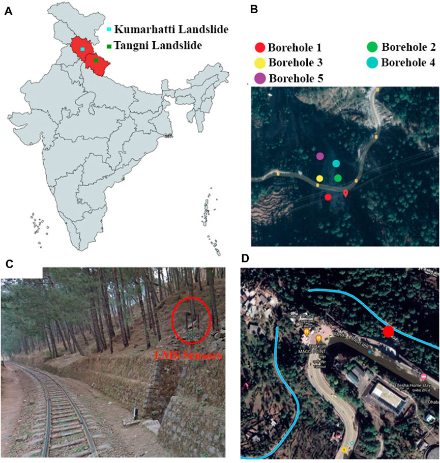
FIGURE 1. (A) Locations of the study areas. (B) Borehole location of the Tangni site on Google Maps. (C) The landslide monitoring sensors installed on a hill near the railway track at Kumarhatti. (D) The Kumarhatti site’s location on Google Maps.

The Kumarhatti site is located in the Solan district, India, along the Kalka - Shimla railway track. The site is at longitude 77° 02′ 50.0″ E and latitude 30° 53′ 37.0″ N at an elevation of 1734 m (Figures 1C,D). The landslide debris often damaged the Kalka - Shimla railway line, which was recorded at the Kumarhatti site by the railway department (Surya, 2011; Chand, 2014). A low cost landslide monitoring system was setup in 2020 at the Kumarhatti site to detect soil movements (Pathania et al., 2020; see Figure 1C).

Soil movement data were collected daily between July 1st, 2012 and July 1st, 2014, from the sensors installed at the Tangni site (see Figure 1B). Soil movement data (in meter) was recorded from the accelerometer sensors installed at the Kumarhatti site between September 10th, 2020, and June 17th, 2021. The accelerometer sensors were installed at 1 m depth from the hill surface at the Kumarhatti site.

Methodology

Data Preparation and Analysis

Tangni Site

The soil movement time series of the Tangni site was collected from several inclinometer sensors. Twenty five inclinometer sensors (i.e., five sensors each at different depths in a borehole across five boreholes) were placed at the Tangni site.

In each borehole, the first sensor was installed at 3 m depth; the second sensor was installed at 6 m; the third sensor was installed at 9 m; the fourth sensor was installed at 12 m; and, the fifth sensor was installed at 15 m depth from the hill’s surface. The sensor measured the inclination change in millimeters per meter (i.e., tilt angle). Figure 2A depicts the working principal of the inclinometer sensor at the site. As illustrated in Figures 2A if the an inclinometer’s length is $L$ and the incline changes by (θ), then the soil movement in $L\cdot \sin \theta$. As a result, we converted soil movement units into inclination $mm/m$ units, where one $mm/m$ unit equaled the 0.057° movement in the soil.

FIGURE 2

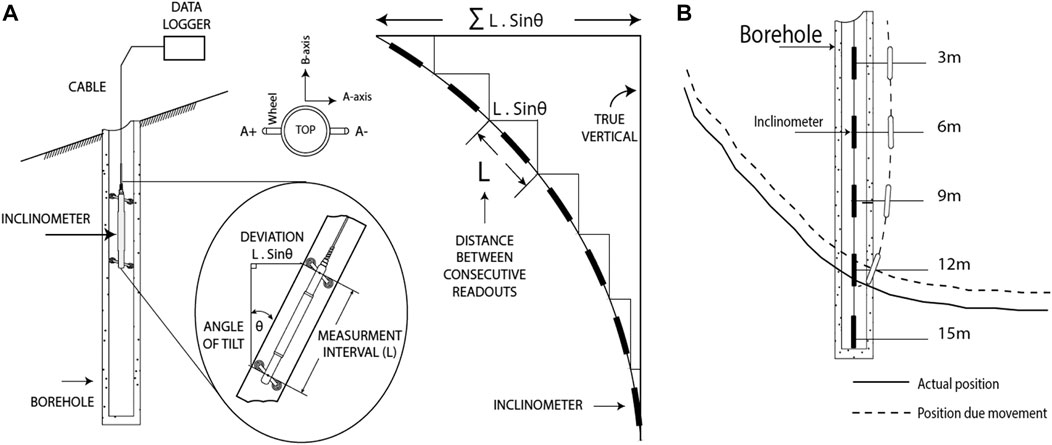
FIGURE 2. (A) The inclinometer sensor was installed in the borehole at the landslide location. (B) The analysis of the maximum soil movement of inclinometer installed at 12 m depth near the failure plane.

As shown in Figure 2A, the sensor has A and B axes, with positive and negative side on each. For example, in the A-axis, the $A^{+}$ side measured the upside movement, and $A^{-}$ side measured downside movement of the hill. The sensors were set up so that the positive A-axis was recording the upward movements and the negative A-axis was recording the downward movements towards the road level.

First, we determined each sensor’s relative tilt angle along the A-axis from its original value at installation time. Second, the sensors closest to the failure plane of the landslide were projected to yield the most significant tilt. As a result, if the sensor is nearby or close to the failure plane, the soil mass movement will be most significant at this sensor (see Figure 2B). We chose those sensors that revealed the maximum soil movement in each borehole over 2 years. As shown in Figures 2A,B sensor in borehole two at a depth of 12 m showed the maximum soil movement over 2 years.

Perhaps, this maximum soil movement was due to the sensor installed near the failure plane in borehole two at a depth of 12 m. Overall, we took the sensor with the maximum average change in inclination from each borehole. As a result, the data set was reduced to five soil movement time series data (captured by a single sensor in each borehole).

Furthermore, there were no soil movements in the daily data. We summed the movement data over a 7 days week to produce 78 weeks of aggregated soil movement data. The weekly time series of five sensors (one in each borehole) were used to develop different RNN models.

Figure 3A–E plots the soil movements (in°) over 78 weeks in each of the five boreholes at Tangni. As illustrated in Figures 3A–E, upward and downward soil movements along the hill were represented by positive and negative tilt angles, respectively. For example, in Figure 3A, in week 30, the movement was 1.71° which changed to −5.53° in week 32. Therefore, there was a rapid downward soil movement of −7.24° in week 32. The soil movement data from borehole one to borehole five showed a consistent downward soil movement behavior (see Figures 3A–E). The borehole one continuously showed a downside soil movement from week one to week 31; but, it showed a considerable movement in week 32. Borehole five, which was installed near the crest, also showed movements between weeks 1 and 78; but, it showed significant movements in weeks 23 and weeks 60–78. Boreholes two, three, and four, located between the crest and toe, detected small soil movement in the beginning and last weeks.

FIGURE 3

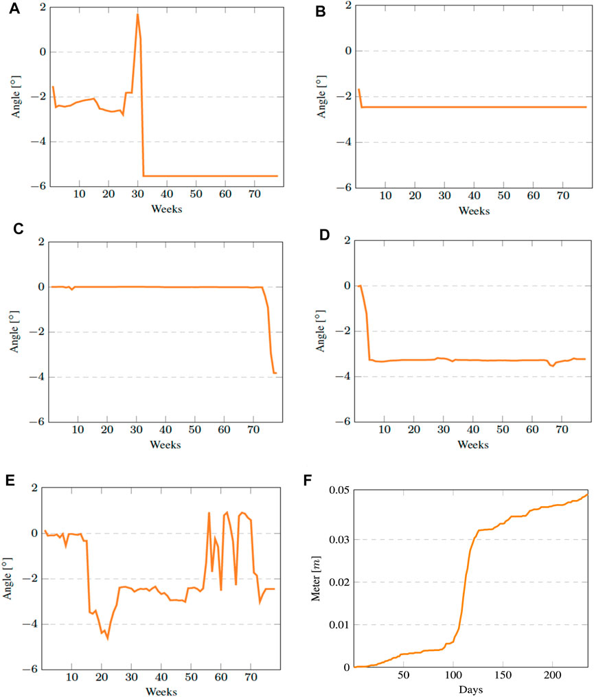
FIGURE 3. The plots of soil movement recorded from sensors deployed at different sites. (A) Sensor tilt at 3 m in borehole one at Tangni. (B) Sensor tilt at 12 m in borehole two at Tangni. (C) Sensor tilt at 6 m in borehole three at Tangni. (D) Sensor tilt at 15 m in borehole four at Tangni. (E) Sensor tilt at 15 m in borehole five at Tangni. (F) Soil movements (in meters) per day at Kumarhatti.

Kumarhatti Site

The landslide monitoring station at the Kumarhatti site has an accelerometer sensor installed at the 1-m depth from the soil’s surface. The sensor has three orthogonal axes, X, Y, and Z, with positive and negative directions on each axis. For example, the X-axis has a positive (X+) side measuring the downside hill movement and a negative (X−) side measuring the upside hill movement. The sensor was installed with X-axis (X+) parallel to the hill’s slope and recorded the positive and negative movements. Every 10 min, the accelerometer sensor recorded the acceleration due to gravity at the deployment. This acceleration was later converted into the soil movements (in meters) at the site by double integration using the trapezoidal rule. The Kumarhatti dataset has 36,000 soil movement points every 10 min over 250 days.

Figure 3F depicts the daily soil movement (in meters) over 250 days for the Kumarhatti dataset. As illustrated in Figure 3F, the positive slope of the soil movement in the graph represents the slope moving toward the railway track at the Kumarhatti site.

The soil movement data from the Tangni and Kumarhatti sites were split into 80 and 20% ratios to train and test different models. For both sites, the developed LSTM models were first trained on the initial 80% training dataset, and they were later tested on the remaining 20% testing dataset. The Tangni dataset has 62 data points for training and 16 for testing. The Kumarhatti dataset has 32,800 data points for training and 7,200 data points for testing.

Dataset Attributes

The Tangni and Kumarhatti datasets included four distinct attributes: the timestamp, the borehole number, the sensor depth, and the soil movement. For example, for Tangni dataset, [2, 2, 12, 1.8°] denotes that the sensor in borehole two at a depth of 12 m recorded the soil movement of 1.8° in the upward direction during the second week since deployment. For Kumarhatti dataset, [20, 1, 1, 0.001 m] denoted that the accelerometer at 1-m depth in borehole one showed the downward movement of 0.001 m in the 200th minute since deployment.

Means, Standard Deviations, and Correlations in the Dataset

Table 1 displays the mean and standard deviation (SD) in the Tangni and Kumarhatti datasets. For example, soil movements in borehole one had an SD of 1.83°. Furthermore, in Table 1, columns three through seven show the correlation value (r) of soil movements between different boreholes at Tangni. The correlation value between boreholes shows that if two boreholes are on the same failure plane of the landslide, both will simultaneously show soil movements with a high correlation. For example, borehole two was highly correlated with borehole four. As shown in Figure 1B, both boreholes are nearby, and it could be possible that both were on the same failure plane. The mean value of the soil movement for the Kumarhatti data was 0.02 m and had a standard deviation of 0.02 m. In Table 1, the borehole is denoted by BH.

TABLE 1

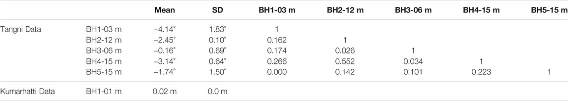
TABLE 1. Means, standard deviations, and the correlations between the time series of different boreholes.

Autocorrelation Plots

The current values within the time series data may correlate to their previous values, which we call lags or look-back periods. The autocorrelation function (ACF) determines the number of lags present in a time series data. The partial autocorrelation function (PACF) determines a direct correlation between the current value and its lag values, removing the correlation of all other intermediate lags. As a result, the ACF value determines how many past forecasted errors are required to forecast the current value, and the PACF value determines how many past forecasted values are required to forecast the current value for the time series data. Figure 4A-4 L show the ACF and PACF plots with a 95% confidence interval for the Tangni and Kumarhatti datasets. As can from these figures, we can see that for the Tangni dataset, the time series one had an ACF value of five and a PACF value of one. The time series two had ACF and PACF values of zero, respectively. The time series three and four had ACF and PACF values of two, respectively. Furthermore, time series five had an ACF value of four and a PACF value of one. Similarly, the time series from the Kumarhatti dataset had an ACF value of forty-two and a PACF value of one. Based upon the range of ACF and PACF values across the two datasets, the look-back period for the developed models was varied from one to five for the Tangni data and one to forty-two for the Kumarhatti data.

FIGURE 4

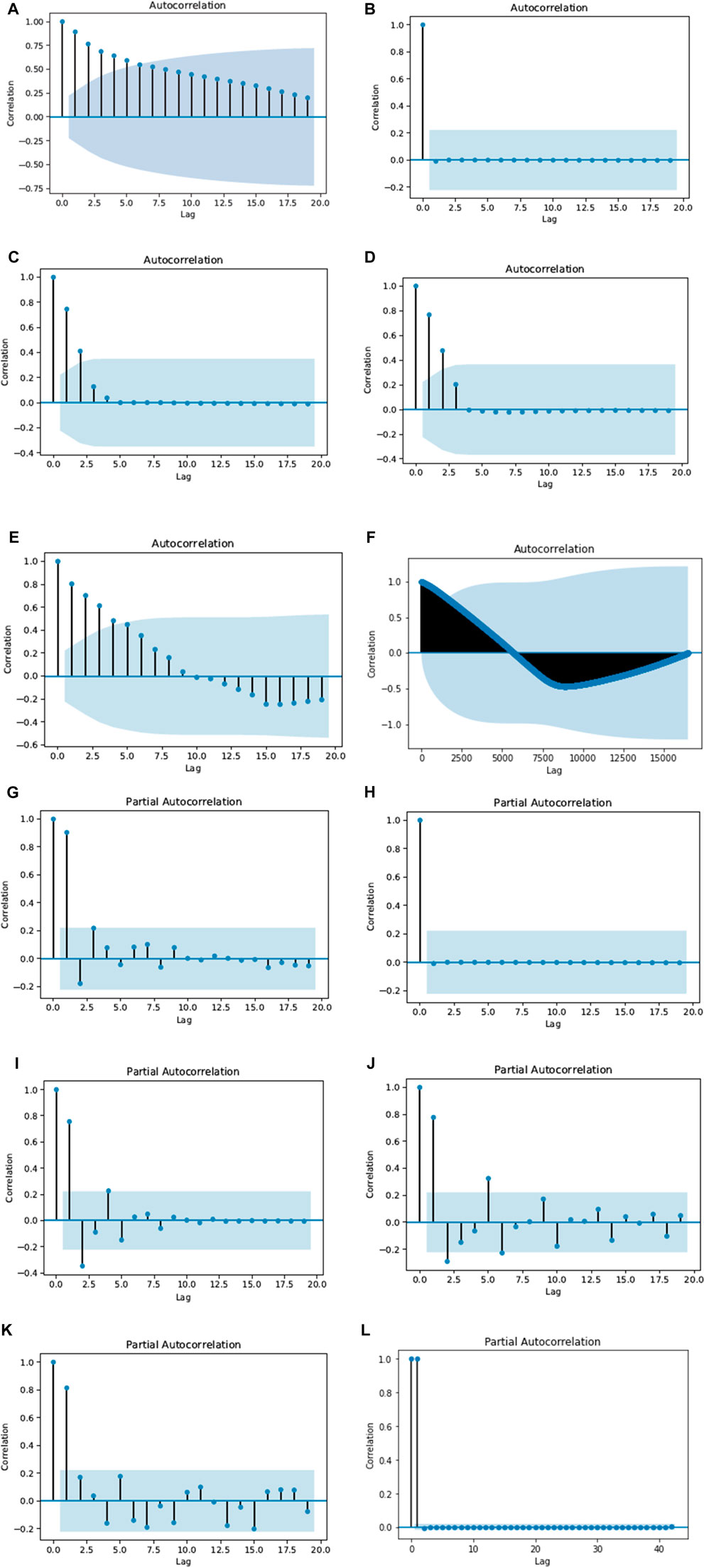
FIGURE 4. The autocorrelation and partial autocorrelation plots with the 95% confidence interval. (A) Autocorrelation for sensor at 3 m in borehole one at Tangni. (B) Autocorrelation for sensor at 12 m in borehole two at Tangni. (C) Autocorrelation for the sensor at 6 m in borehole three at Tangni. (D) Autocorrelation for the sensor at 15 m in borehole four at Tangni. (E) Autocorrelation for the sensor at 15 m in borehole five at Tangni. (F) Autocorrelations for the Kumarhatti data. (G) Partial autocorrelation for the sensor at 3 m in borehole one at Tangni. (H) Partial autocorrelation for the sensor at 12 m in borehole two at Tangni. (I) Partial autocorrelation for the sensor at 6 m in borehole three at Tangni. (J) Partial autocorrelation for the sensor at 15 m in borehole four at Tangni. (K) Partial autocorrelation for the sensor at 15 m in borehole five at Tangni. (L) Partial autocorrelations for the Kumarhatti data.

Recurrent Neural Network Models

Recurrent neural networks (RNNs) are specially designed to discover dependencies between current and previous values in time series data (Medsker and Jain, 1999). RNN networks are composed of a chain of cells linked by a feedback loop, and these cells extract temporal information from time series data. In general, every cell in RNNs has a simple design, such as a tanh function (Medsker and Jain, 1999). In general, the RNN models suffer from the exploding and vanishing gradients problem during the training process (Bengio et al., 1994). The problem arises when the long sequence of small or large values multiplies while calculating the gradient in the backpropagation. The exploding and vanishing gradient problems in the RNN model prevent the model from learning the long-term dependency in the data.

LSTMs solve the exploding and vanishing gradient problems by employing a novel additive gradient structure in the backpropagation. The additive gradient structure includes direct access to the forget gate activations, allowing the network to update its parameters so that the gradient does not explode or vanish (Hochreiter and Schmidhuber, 1997). Thus, LSTMs solve the problem of vanishing gradient and the learning of longer-term dependencies in RNNs models.

Simple Long Short-Term Memory Model

The simple LSTM is a type of RNN model that can remember values from previous stages (Medsker and Jain, 1999). The cell state in an LSTM acts as a conveyor belt $\left(c^{<t>}\right)$, allowing unaltered information to flow through the units with only a few linear interactions. The internal architecture of each LSTM unit has an input gate $\left(i^{<t>}\right)$, forget gate $\left(f^{<t>}\right)$, and output gate $\left(o^{<t>}\right)$. These three gates control the flow of information and avoid the exploding or vanishing gradient problems during training (Hochreiter and Schmidhuber, 1997) (see Figure 5A). The input gate adds new information from the new input and previous output to the cell state. The forget gate determines what information is retained for a long time and what information is removed from the cell state. The forget gate uses the sigmoid (logistic) function, where the sigmoid function’s output value is between zero and one. The forgot gate’s output zero means to remove the information from the cell state, and output one means to keep the information. The purpose of the output gate is to determine what output value its required from the cell state, and the output gate also updates the previous state of the hidden state $\left(h^{<t-1>}\right)$. There is also a layer in the LSTM unit that contains the tanh activation function, which is used to update the state of neurons (see Figure 5A). Eqs 1–5 are the fundamental equations of the LSTM cell, with the Hadamard product denoted by the letter ′$o$′:

$i^{<t>}=\sigma \left(W_{xi}{x}_t+W_{hi} h^{<t-1>}+W_{ci}o{c}^{<t-1>}+b_i\right)(1)$

$f^{<t>}=\sigma \left(W_{xf}{x}_t+W_{hf} h^{<t-1>}+W_{cf}o{c}^{<t-1>}+b_f\right)(2)$

$c^{<t>}=i^{<t>}o{c}^{<t-1>}+i^{<t>}otanh\left(W_{xc}{x}_t+W_{hc }{h}^{<t-1>}+b_c\right)(3)$

$o^{<t>}=\sigma \left(W_{xo}{x}_t+W_{ho} h^{<t-1>}+W_{co}o c^{<t-1>}+b_o\right)(4)$

$h^{<t>}=o^{<t>}otanh\left(c^{<t>}\right)(5)$

Where, $i^{<t>}$ is the input gate at timestamp t; $f^{<t>}$ is the forgot gate at timestamp t; $c^{<t>}$ is the cell state at timestamp t; $o^{<t>}$ is the output gate at timestamp t; and $h^{<t>}$ is the hidden state at timestamp t. The variable x_t in the equations represents the input data sequence at timestamp t. The matrices $W_{xi}$, $W_{ci}, W_{xf}, W_{hf}, W_{cf}, W_{xc}, W_{hc}, W_{xo}, W_{ho},$ and $W_{co}$ are the weight matrices between two different layers. For example, the $W_{xi}$ is the weight matrix between input data sequence x and input gate $i^{<t>}$. Similarly, the $b_i$, $b_f, b_o,$and $b_c$ are the biases for the input gate, forgot gate, output gate, and cell state, respectively. The $tanh$ and $\sigma$ here represent the tan hyperbolic and sigmoid (logistic) activation functions.

FIGURE 5

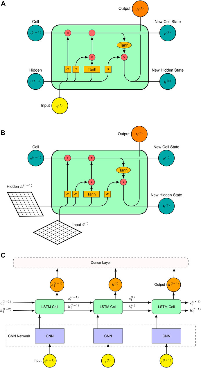
FIGURE 5. (A) A layer of the simple LSTM with three gates. (B) A Conv-LSTM model with a convolution operation on input and hidden state. (C) A CNN-LSTM with a CNN network at an input layer.

Convolutional Long Short-Term Memory Model

Conv-LSTM is a combination of convolution operation of the CNN model and the LSTM model (Shi et al., 2015). As shown in Figure 5B, the convolution operation is applied to the input and the hidden state of the LSTM cells. As a result, at each gate of the LSTM cell, the internal matrix multiplication process is changed by the convolution operation (*). This operation can find the underlying spatial information in high-dimensional data. The Conv-LSTM’s critical equations are provided in Eqs 6–10 below, where the convolution operation is denoted by ′*′ and the Hadamard product is denoted by ′$o$′:

$i^{<t>}=\sigma \left(W_{xi}\text{*}{x}_t+W_{hi} \text{*}{h}^{<t-1>}+W_{ci}o{c}^{<t-1>}+b_i\right)(6)$

$f^{<t>}=\sigma \left(W_{xf}\text{*}{x}_t+W_{hf} \text{*}{h}^{<t-1>}+W_{cf}o{c}^{<t-1>}+b_f\right)(7)$

$c^{<t>}=i^{<t>}o{c}^{<t-1>}+i^{<t>}otanh\left(W_{xc}\text{*}{x}_t+W_{hc}\text{*}{h}^{<t-1>}+b_c\right)(8)$

$o^{<t>}=\sigma \left(W_{xo}\text{*}{x}_t+W_{ho}\text{*}{h}^{<t-1>}+W_{co}o{c}^{<t-1>}+b_o\right)(9)$

$h^{<t>}=o^{<t>}otanh\left(c^{<t>}\right)(10)$

Where, $i^{<t>}$ is the input gate at timestamp t; $f^{<t>}$ is the forgot gate at timestamp t; $c^{<t>}$ is the cell state at timestamp t; $o^{<t>}$ is the output gate at timestamp t; and $h^{<t>}$ is the hidden state at timestamp t. The variable x_t in the equations represents the input data sequence at timestamp t. The matrices $W_{xi}$, $W_{ci}, W_{xf}, W_{hf}, W_{cf}, W_{xc}, W_{hc}, W_{xo}, W_{ho},$ and $W_{co}$ are the weight matrices between two different layers. Similarly, the $b_i$, $b_f, b_o,$and $b_c$ are the biases for the input gate, forgot gate, output gate, and cell state, respectively. The $tanh$ and $\sigma$ here represent the tan hyperbolic and sigmoid (logistic) activation functions.

CNN-Long Short-Term Memory Model

The CNN-LSTM model is an ensemble of CNN and LSTM models (Wang et al., 2016). As shown in Figure 5C, the CNN model first searches for spatial information in high-dimensional input data and transforms it into one-dimensional data. The one-dimensional data is then fed as an input to the LSTM model. Here the CNN network acts as a spatial feature extractor.

Bidirectional Long Short-Term Memory (Bi-Long Short-Term Memory) Model

This model is mainly designed to improve the performance of the simple LSTM model. The Bi-LSTM model trains the two parallel LSTM layers simultaneously (Cui et al., 2018). The models train one of the parallel layers in the forward direction of the input data and another layer in the backward direction of the input data (see Figure 6A). The Bi-LSTM model could learn more patterns from the input data than the simple LSTM model in this forward and backward training method. As the input data grows, the Bi-LSTM model identifies the unique pieces of information from the data.

FIGURE 6

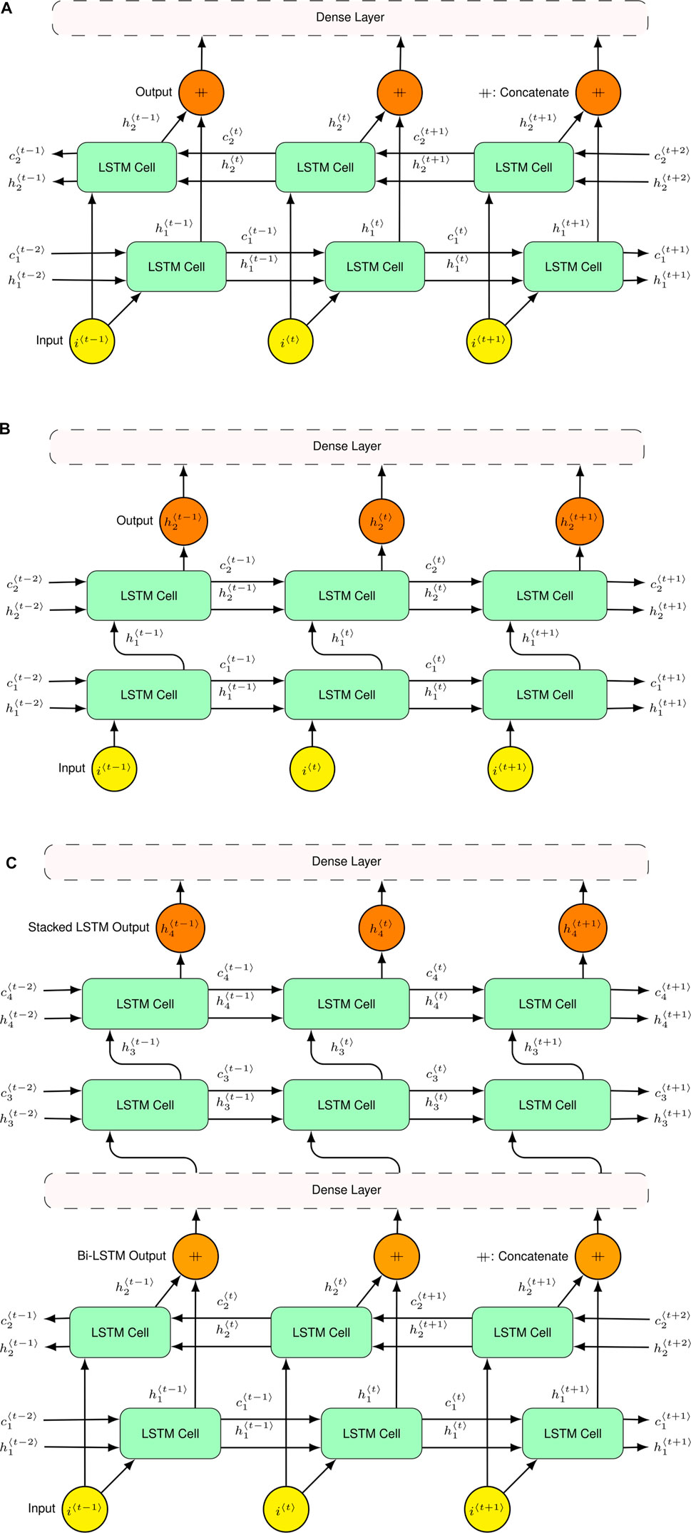
FIGURE 6. (A) The structure of the Bi-LSTM. (B) The structure of a two-layer stacked LSTM. (C) The structure of the BS-LSTM.

Figure 6A depicts the Bi-LSTM design, which consists of two simple LSTM layers. One layer of the model trains the model forward, while a second layer of the LSTM trains the model backward. The parallel layers of the LSTM model receive the same input data and combine their outputs as one output. Finally, in order to forecast the output, the Bi-LSTM model is linked to a dense layer.

Stacked Long Short-Term Memory Model

The stacked LSTM could be developed by stacking the two simple LSTM layers. The first layer receives the input from the input layer and provides the input to the next connected LSTM layer (see Figure 6B) (Yu et al., 2019). Stacking multiple LSTM layers on top of each other allows the model to learn different temporal patterns from various timestamps in the input data. This design gives more power to the LSTM models to converge faster.

Figure 6B shows a stacked LSTM with two layers stacked on top of each other. The first layer of the stacked LSTM model is designed to take data from the input layer and process it before passing it to the next layer. The next layer is linked to the dense layer, which processes the output of the first layer before passing it to the dense layer. Finally, the dense layer forecasts the required outputs. The primary equations of the model, which update the model’s initial layer, are as follows:

$i_l^{<t>}=\sigma \left(W_l^{xi}{h}_{l-1}^{<t>}+W_l^{hi}{h}_l^{<t-1>}+W_l^{ci}o{c}_l^{<t-1>}+b_l^i\right)(11)$

$f_l^{<t>}=\sigma \left(W_l^{xf}{h}_{l-1}^{<t>}+W_l^{hf}{h}_l^{<t-1>}+W_l^{cf}o{c}_l^{<t-1>}+b_l^f\right)(12)$

$c_l^{<t>}=f_l^{<t>}o c_l^{<t-1>}{i}_l^{<t>}otanh\left(W_l^{xc}{h}_{l-1}^{<t>}+W_l^{hc}{h}_l^{<t-1>}+b_l^c\right)(13)$

$o_l^{<t>}=\sigma \left(W_l^{xo}{h}_{l-1}^{<t>}+W_l^{ho}{h}_l^{<t-1>}+W_l^{co}o{c}_l^{<t-1>}+b_l^o\right)(14)$

$h_l^{<t>}=o_l^{<t>}otanh\left(c_l^{<t>}\right)(15)$

Where, the variable x_t in the equations is representing the input data sequence at timestamp t. The matrices $W_l^{xi}$, $W_l^{ci}, W_l^{xf}, W_l^{hf}, W_l^{cf}, W_l^{xc}, W_l^{hc}, W_l^{xo}, W_l^{ho},$ and$W_l^{co}$ are the weight matrices between two different layers at the level l. Similarly, the $b_l^i$, $b_l^f, b_l^o,$and $b_l^c$ are the biases at the level l for the input gate, forgot gate, output gate, and cell state, respectively.

Bidirectional Stacked Long Short-Term Memory Model

An ensembled version of a bidirectional LSTM and a stacked LSTM (called the BS-LSTM network) is a newly designed model for sequence forecasts. A bidirectional LSTM network is concatenated with a stacked LSTM network (see Figure 6C). First, the bidirectional LSTM network is trained in both directions of the input time series (week one to week 62 and vice versa). Second, the output of the bidirectional LSTM layers is linked to a dense layer. Next, the dense layer’s output is provided as input to the stacked LSTM layers. Finally, the stacked LSTM layers relate to a dense layer. The final dense layer forecast the required outputs.

As seen in Figure 6C, seven layers make up the structure of the BS-LSTM model. The input layer was the first layer, and the following two parallel layers were trained in the forward and backward directions. Next, the output of the Bi-LSTM model was related to the dense layer. The dense layer provided the values to the input layer of the stacked LSTM. In the design of this stacked LSTM, two LSTM layers were stacked, one on top of the other. The output of the last stacked layer was related to the dense layer. Finally, the dense layer of the stacked LSTM forecasted the following week’s soil movements.

Model Parameters Tuning

The first layer in different models was the input layer. The input layer’s dimension could be determined by the features in the dataset, look-back periods, and batch size. The Tangni dataset had fewer data points than Kumarhatti. Thus, the batch size was selected as 16 for Tangni and 1,024 for Kumarhatti. The range of the look-back periods was estimated from the ACF and PACF values. As per the ACF and PACF values, the look-back period for the Tangni dataset was varied from one to five. Similarly, the look-back period for the Kumarhatti dataset was varied from one to forty-two. The number of the features in both datasets was three (i.e., borehole, depth, and soil movement). The second layer was the hidden layer. The nodes in the hidden layer of the LSTM models are called LSTM units. In this research, the one-step forecasting method has been used to forecast the soil movement at the next timestamp.

Simple Long Short-Term Memory Model

The number of LSTM units in the hidden layer was changed between 1 and 400 with a step size of 50. The hidden layer’s output vector size was the same as the number of LSTM units in this layer. The dimension of the model’s output could be changed by a dense layer. The dense layer consists of several neurons with a linear activation function. The dense layer’s output vector size was the same as the number of neurons in this layer. Thus, the dense layer with one neuron was connected to the last hidden layer. Table 2 shows the various parameters used by this model to forecast the soil movement in the Tangni and Kumarhatti datasets.

TABLE 2

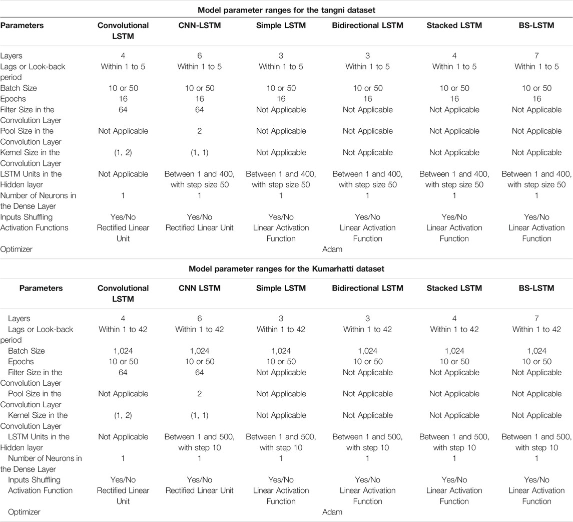
TABLE 2. Parameter optimization of different LSTM models.

Conv-Long Short-Term Memory Model

In this model, the output dimension of the convolution layer was determined by the batch size, new number of rows, new number of columns, and the number of filters. In the convolution layer, the batch size was selected as 16 for Tangni and 1,024 for Kumarhatti. The new number of rows and columns were set as one and two, respectively. The number of filters was selected as 62. The kernel size of the convolution layer was set to $1\times 2$. The output vector dimension of the convolution layer was multidimensional, so a flatten layer was added after the convolution layer. The flatten layer converted the multidimensional data into one dimension. The dimension of the model’s output could be changed by a dense layer. The dense layer consists of several neurons with a rectified linear unit (ReLU) activation function. The dense layer’s output vector size was the same as the number of neurons in this layer. Thus, the dense layer with one neuron was connected to the last hidden layer. Table 2 shows the various parameters used by this model to forecast the soil movements in the Tangni and Kumarhatti datasets.

CNN-Long Short-Term Memory Model

In this model, the time distributed convolution layer executed the same convolution operation to each timestamp as the LSTMs unrolled. The output dimension of the convolution layer was determined by the batch size, new number of rows, new number of columns, and the number of filters. In the convolution layer, both new rows and columns were set as one. The number of filters was selected as 62. The kernel size of the convolution layer was set to $1\times 1$. A max-pooling layer was used to reduce the spatial dimensions. The pool size of the max-pooling layer was set at 2. The max-pooling layers’ output was multidimensional, so a flatten layer was added after the max-pooling layer. The flattening layer converted the multidimensional data into one dimension. The flatten layer provided the one-dimensional data to the next hidden layer. The next layer was the hidden layer. The nodes in the hidden layer are called LSTM units. The number of LSTM units in the hidden layer was changed between 1 and 400 with a step size of 50. The hidden layer’s output vector size was the same as the number of LSTM units in this layer. The dimension of the model’s output could be changed by a dense layer. The dense layer consists of several neurons with a rectified linear unit (ReLU) activation function. The dense layer’s output vector size was the same as the number of neurons in this layer. Thus, the dense layer with one neuron was connected to the last hidden layer. Table 2 shows the various parameters used by this model to forecast the soil movements in the Tangni and Kumarhatti datasets.

Bi-Long Short-Term Memory Model

In this model, the nodes in the hidden layer was called LSTM units. The number of LSTM units in both hidden layers was changed simultaneously between 1 and 400 with a step size of 50. The hidden layer’s output vector size was the same as the number of LSTM units in this layer. The dimension of the model’s output could be changed by a dense layer. The dense layer consists of several neurons with a linear activation function. The dense layer’s output vector size was the same as the number of neurons in this layer. In this research, the one-look-ahead forecasting method has been used. Thus, the dense layer with one neuron was connected to the last hidden layer. Table 2 shows the various parameters used by this model to forecast the soil movements in the Tangni and Kumarhatti datasets.

Stacked Long Short-Term Memory Model

In this model, the number of LSTM units in the hidden layer was changed between 1 and 400 with a step size of 50. The hidden layer’s output vector size was the same as the number of LSTM units in this layer. The dimension of the model’s output could be changed by a dense layer. The dense layer consists of several neurons with a linear activation function. The dense layer’s output vector size was the same as the number of neurons in this layer. Thus, the dense layer with one neuron was connected to the last hidden layer. Table 2 shows the various parameters used by this model to forecast the soil movements in the Tangni and Kumarhatti datasets.

BS-Long Short-Term Memory Model

This model has seven layers, three in the Bi-LSTM model (Input: one; Hidden: one; Output:1) and four in the stacked LSTM model (Input: one; Stacked: two; Output:1). The architecture of the Bi-LSTM and stacked LSTM layers was the same as Bi-LSTM and stacked LSTM model developed in this paper. Table 2 shows the various parameter values used by this model to forecast the soil movement in the Tangni and Kumarhatti datasets. For example, the BS-LSTM parameters for the Tangni dataset were varied as per the following: the batch size was fixed at 16; the LSTM units in the hidden layers were selected between 1 and 400 with a step size of 50 for the Bi-LSTM model and changed between 1 and 400 with a step size of 50 for both stacked layers in stacked LSTM; the number of epochs was changed as 10 or 50; the look-back period was varied from one to five; and, the inputs were passed with shuffling turned on or turned off. The BS-LSTM parameters for the Kumarhatti dataset were varied as per the following: the batch size was fixed at 1,024; the hidden layer’s LSTM units in Bi-LSTM and stacked LSTM were varied between 1 and 500 with a step size of 10; the number of epochs was changed as 10 or 50; the look-back period was varied between 1 and 42 (as estimated from ACF and PACF); and, the inputs were passed with shuffling and without shuffling.

Model’s Inputs and Outputs

Before entering the time series data into models, we divided the input data into several packets based on borehole and depth. Packets from the first 80% of data were utilized to training the models, and packets from the last 20% of data were used for testing the models. Each packet was a combination of X, Y, where X was the predictor, and Y was the forecasted soil movement value (see Figure 7). As shown in Figure 7, the X predictor formed a movement vector consisting of soil movements recorded by a sensor in a borehole in a timestamp (M), borehole number of the sensor (Borehole), and the depth of the sensor (Depth). The M was the timestamp value of the soil movement recorded by a sensor in a borehole in a particular time. The Borehole value was one of the five boreholes at the site. The Depth value was the depth of the sensor in a specific borehole. For example, for a look-back period of three in the Tangni dataset, packet X₁ may contain the movement recorded by the sensor in the first 3 weeks in borehole one at a depth of 3 m. The corresponding Y₁ contained the actual value of the movement recorded by the same sensor in borehole one in week four, forecasted by a model. Thus, there was a one-look-ahead soil movement forecast (Y) for a certain look-back period and for a particular sensor at a specific depth (X) (the look-back was passed to models as a parameter). These X and Y packets could be shuffled before input to a model, where the shuffle operation would shuffle the two lists (i.e., X and Y) in the same order (see Figure 7).

FIGURE 7

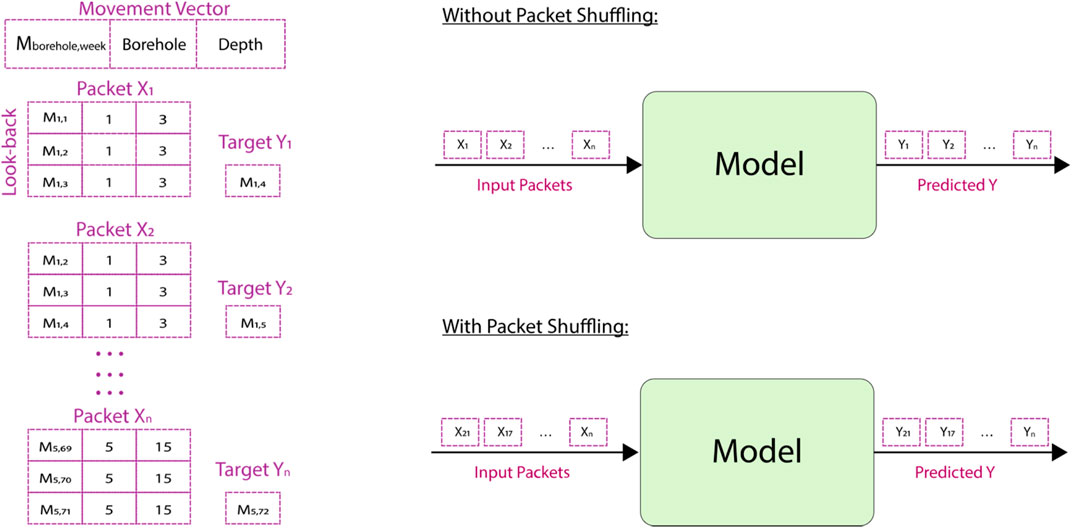
FIGURE 7. Inputs and outputs in a model.

Dropouts in Models

The Tangni dataset has a limited amount of data, where the training dataset has only 62 data points to train LSTM models. When the training dataset is limited, the system can overfit the model’s parameters during training. The dropouts can be applied to the layers of the LSTM to prevent overfitting (Pham et al., 2014; Gal and Ghahramani, 2016). Different combinations with the probability (p) of dropout were applied on the input-output and recurrent connections of the LSTM layer. The probability value (p) was varied between 0.0 and 0.8 with step size 0.2, where a p-value of 0.0 means no dropout applied. For example, a combination (0.2, 0.8) represents 20% dropout applied to the LSTM unit’s output and 80% dropout applied on the recurrent input of the LSTM unit (Gal and Ghahramani, 2016).

Performance Measure for the Models

The soil movement forecasting is a regression problem, where the resulting soil movement is assumed to have a floating value. Thus, an error can be calculated between the true value and the forecasted value of the soil movements. The different performance measures have been used to evaluate the performance measure of the various models (Behera et al., 2018). In this paper, four performance measures are used: mean relative error (MRE), root mean square error (RMSE), normalized root mean squared error (NRMSE), and mean absolute error (MAE). Eqs 16–19 were used to calculate the values of these measures to find the difference between actual points of datasets from the forecasted points of datasets.

$RMSE=\sqrt{\frac{1}{n}{\displaystyle \sum }_{i=1}^n{\left(Trueangle-Forecastedangle\right)}^2}(16)$

$NRMSE=\frac{\sqrt{{\Sigma }_{i=1}^n{\left(Trueangle-Forecastedangle\right)}^2}}{{\Sigma }_{i=1}^n{\left(Forecastedangle\right)}^2}(17)$

$MAE=\frac{1}{n}{\displaystyle \sum }_{i=1}^n\left(\left|Trueangle-Forecastedangle\right|\right)(18)$

$MRE=\frac{1}{n}{\displaystyle \sum }_{i=1}^n\left(\left|\frac{Trueangle-Forecastedangle}{Forecastedangle}\right|\right)\text{*}100(19)$

where, n denotes the number of data points in the Tangni or Kumarhatti dataset, the true angle denotes the actual observed value of the soil movements in the dataset, and the forecasted angle denotes the forecasted value of the soil movements by the model.

Model Calibration

We created a grid search procedure to calibrate the parameters in various models. In this process, we changed the different set of parameters (described in Table 2) in a LSTM model. After feeding a combination into the LSTM models, we recorded the MAE, RMSE, NRMSE, and MRE, and we chose the parameters with the lowest error in the model.

Results

The developed LSTM models first trained on the first 80% data and then tested on the remaining 20% data. The training and testing results of these models across the Tangni and Kumarhatti datasets are reported in Table 3. The results in Table 3 are sorted according to the model’s performance (minimum RMSE first) on the testing dataset. As can see in Table 3, the BS-LSTM and Bi-LSTM models outperformed the other models in training and testing across the Tangni and Kumarhatti datasets.

TABLE 3

TABLE 3. Errors of various models in the training and testing dataset.

Table 4 introduces the optimized value of parameters for all models. As can see in Table 4, for the Tangni landslide dataset, the least error of the Bi-LSTM model was at the look-back period = 4, number of epochs = 50, batch size = 16, LSTM units in the hidden layer = 400, with the shuffling of inputs, and no dropouts applied on the LSTM layer. Table 4 shows the optimized values for the BS-LSTM model, where the BS-LSTM model was an ensemble version of two different recurrent models, Bi-LSTM and stacked LSTM. The Bi-LSTM was trained first. The best set of Bi-LSTM parameters that minimized the RMSE on the Tangni dataset included: look-back periods = 4, shuffling turned on, LSTM units in the hidden layer = 400, the number of epochs = 50, batch size = 16, and no dropouts applied on the LSTM layer. Next, the trained Bi-LSTM model’s output forecasted values were fed into a stacked LSTM as an input. The stacked LSTM was trained next, where the minimum RMSE was produced with the following parameters: batch size = 4, number of epochs = 50, packets without shuffled, no dropouts, number of nodes in input layer = 12, number of LSTM units in first stacked layer = 200, second stacked layer = 100, and number of neurons in the dense layer = 1. For the Tangni dataset, most LSTM models had a look-back period of four, as shown in Table 4. Furthermore, the Kumarhatti dataset had a PACF value of one, implying that this time series was only required a single look-back period. As shown in Table 4, most LSTM models had a one-look-back period on the Kumarhatti dataset. The models’ parameters optimization found that the look-back period was the most critical parameter to reduce error.

TABLE 4

TABLE 4. Optimized parameters for the different models on the Tangni and Kumarhatti datasets.

Figure 8 depicts the top-performing BS-LSTM model’s training and test fit over five boreholes from the Tangni site and one borehole from the Kumarhatti site.

FIGURE 8

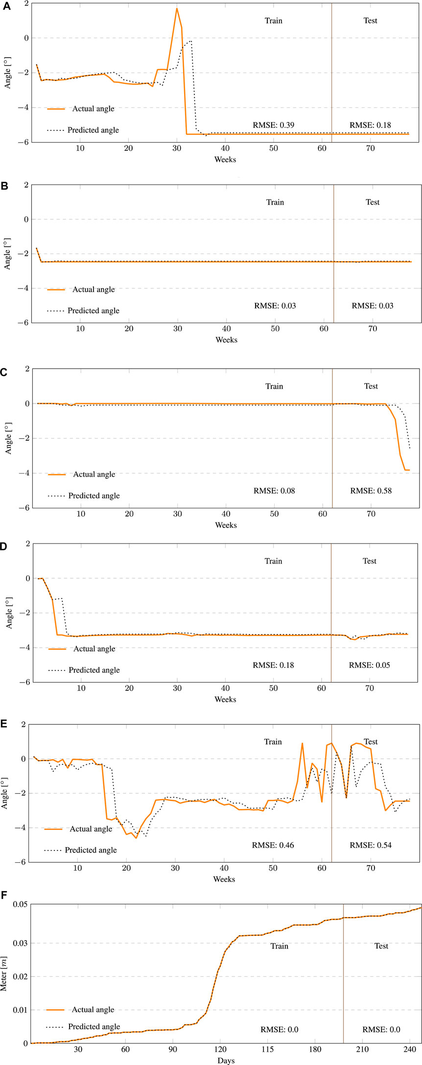
FIGURE 8. The best performing BS-LSTM model showing the soil movements (in degree) over the Tangni landslide training and test datasets. (A) The sensor at 3 m in borehole one at Tangni. (B) The sensor at 12 m in borehole two at Tangni. (C) The sensor at 6 m in borehole three at Tangni. (D) The sensor at 15 m in borehole four at Tangni. (E) The sensor at 15 m in borehole five at Tangni. (F) The best performing BS-LSTM model showing the soil movement (in meters) over the Kumarhatti’s training and testing datasets.

Discussion and Conclusion

A focus of recurrent neural network models could be the forecasting of soil movements to warn people about impending landslides. We developed a novel ensemble BS-LSTM model (a combination of a Bi-LSTM model and a stacked LSTM model). We calibrated the parameters of the BS-LSTM model on the Tangni and Kumarhatti datasets. The soil movement data from the Tangni and Kumarhatti were split into 80 and 20% ratios to train and test the LSTM models. The developed LSTM models first trained on the initial 80% training dataset with a one-step look ahead forecasting method and later tested on the remaining 20% testing dataset for both locations. Four performance measures MAE, RMSE, NRMSE, and MRE, were utilized to record the performance of the models.

For the Tangni and Kumarhatti datasets, the ensemble BS-LSTM was the best model to forecast the soil movements during model training and testing. The Bi-LSTM was the second-best model to forecast the soil movements for both datasets. An explanation for the BS-LSTM’s performance might be that the inbuilt Bi-LSTM found more information in the input time series via training the model in both forward and backward directions. Next, the inbuilt stacked LSTM could utilize this information to forecast the soil movement values.

Another observation from this experiment that the LSTM models trained on the Tangni landslide dataset showed some overfitting, where the training error was less than the testing error. The one reason could be that the LSTM models have memory limitations in general. The LSTM models require more data to train their parameters, where the Tangni dataset has only 62 data points. The LSTM models were trained on the Kumarhatti dataset to investigate the memory limitations, and the results were reasonably good without overfitting. During the training and testing of the Kumarhatti dataset, the LSTM models showed almost no error in the soil movement forecasting.

The LSTM models in this paper were developed to forecast the sequence of soil movements. The CNN-LSTM and Conv-LSTM models were developed by ensembling of the CNN network and a simple LSTM model. The ensembling fed the spatial information of soil movements into the simple LSTM model, which increased the performance of these models. The developed Bi-LSTM and stacked LSTM models were the non-ensemble models. The BS-LSTM model was developed using the Bi-LSTM and stacked LSTM models. The BS-LSTM was compared with an ensemble of CNN and simple LSTM models (CNN-LSTM and Conv-LSTM) to forecast soil movements on the Tangni and Kumarhatti datasets. The training and test results demonstrated that the BS-LSTM models outperformed the ensemble of CNN and simple LSTM models.

Results reported in this paper have several implications for soil movement forecasts in the real world. First, the results show that an ensemble of RNN models (such as BS-LSTM) could be utilized to forecast soil movements at real-world landslide sites. Our findings show that an ensemble BS-LSTM outperforms the non-ensemble models and ensemble of CNN and simple LSTM models for forecasting of soil movements. Furthermore, this is the first attempt to use recurrent neural network models to model soil movements at the Tangni and Kumarhatti sites. Such an ensemble of recurrent neural networks may also have the scope in other fields such as social network analysis and natural language processing, respectively.

According to this article, recurrent neural network models might be useful in anticipating soil movements to warn people about impending landslides. During the training and testing of the Kumarhatti dataset, the LSTM models showed almost no error in the soil movement forecasting. In conclusion, the newly developed ensemble models were generalized to forecast the soil movements on different landslides. In future, these models could be used to forecast the soil movements at other landslide sites in India and in other countries. The soil movement forecasting is a class imbalance problem where movement events may be lesser than non-movement events. Also, the machine learning models could show overfitting when training data is scarce. In such situations, the generative adversarial networks (GANs) could generate synthetic data of soil movements to solve class imbalance in datasets (Al-Najjar and Pradhan, 2021). For example, Al-Najjar and Pradhan, (2021) developed a GAN model for spatial landslide susceptibility assessment when training data was less. As a part of our future plan, we would like to extend this research by developing various GAN models for soil movement forecasting. A portion of these ideas forms the immediate stages in our project on soil-movement forecasts utilizing machine learning approaches.

Data Availability Statement

The raw data supporting the conclusions of this article will be made available by the authors, without undue reservation.

Author Contributions

PK: Formulation of this study, methodology, and model implementation. PS: Data curation, writing, and original draft preparation. PC: Data collection. KU: Validation of the results and geotechnical parameters. VD: The compilation, examination, and interpretation of data for the work.

Funding

The project was supported by grants (awards: IITM/DST/VKU/300, IITM/DST/KVU/316, and IITM/DDMA-M/VD/325) to VD.

Conflict of Interest

The authors declare that the research was conducted in the absence of any commercial or financial relationships that could be construed as a potential conflict of interest.

Publisher’s Note

All claims expressed in this article are solely those of the authors and do not necessarily represent those of their affiliated organizations, or those of the publisher, the editors and the reviewers. Any product that may be evaluated in this article, or claim that may be made by its manufacturer, is not guaranteed or endorsed by the publisher.

Acknowledgments

We are grateful to the Department of Science and Technology and to District Disaster Management Authority Mandi for providing the funding for this project. We are also grateful to the Indian Institute of Technology Mandi for providing computational resources for this project.

References

Al-Najjar, H. A. H., and Pradhan, B. (2021). Spatial Landslide Susceptibility Assessment Using Machine Learning Techniques Assisted by Additional Data Created With Generative Adversarial Networks. Geosci. Front. 12 (2), 625–637. doi:10.1016/j.gsf.2020.09.002

CrossRef Full Text | Google Scholar

Barzegar, R., Aalami, M. T., and Adamowski, J. (2020). Short-Term Water Quality Variable Prediction Using a Hybrid CNN-LSTM Deep Learning Model. Stoch Environ. Res. Risk Assess. 34, 415–433. doi:10.1007/s00477-020-01776-2

CrossRef Full Text | Google Scholar

Behera, R. K., Naik, D., Rath, S. K., and Dharavath, R. (2019). Genetic Algorithm-Based Community Detection in Large-Scale Social Networks. Neural Comput. Appl., 1–17.

CrossRef Full Text | Google Scholar

Behera, R. K., Naik, D., Ramesh, D., and Rath, S. K. (2020). Mr-ibc: Mapreduce-Based Incremental Betweenness Centrality in Large-Scale Complex Networks. Social Netw. Anal. Mining. 10 (1), 1–13. doi:10.1007/s13278-020-00636-9

CrossRef Full Text | Google Scholar

Behera, R. K., Sahoo, K. S., Naik, D., Rath, S. K., and Sahoo, B. (2021a). Structural Mining for Link Prediction Using Various Machine Learning Algorithms. Int. J. Soc. Ecol. Sustainable Development (Ijsesd). 12 (3), 66–78. doi:10.4018/ijsesd.2021070105

CrossRef Full Text | Google Scholar

Behera, R. K., Jena, M., Rath, S. K., and Misra, S. (2021b). Co-LSTM: Convolutional LSTM Model for Sentiment Analysis in Social Big Data. Inf. Process. Management. 58 (1), 102435. doi:10.1016/j.ipm.2020.102435

CrossRef Full Text | Google Scholar

Behera, R. K., Shukla, S., Rath, S. K., and Misra, S. (2018). Software Reliability Assessment Using Machine Learning Technique. In International Conference on Computational Science and Its Applications. Cham: Springer, 403–411. doi:10.1007/978-3-319-95174-4_32

CrossRef Full Text | Google Scholar

Bengio, Y., Simard, P., and Frasconi, P. (1994). Learning Long-Term Dependencies With Gradient Descent Is Difficult. IEEE Trans. Neural Netw. 5 (2), 157–166. doi:10.1109/72.279181

PubMed Abstract | CrossRef Full Text | Google Scholar

Chand, K. (2014). Spatial Trends and Pattern of Landslides in the Hill State Himachal Pradesh. Zenith Int. J. Multidisciplinary Res. 4 (12), 200–210.

Google Scholar

Chaturvedi, P., Srivastava, S., and Kaur, P. B. (2017). “Landslide Early Warning System Development Using Statistical Analysis of Sensors' Data at Tangni Landslide, Uttarakhand, india,” in Proceedings of Sixth International Conference on Soft Computing for Problem Solving. Editors K. Deep, J.C. Bansal, K.N. Das, A.K. Lal, H. Garg, A.K. Nagaret al. (Singapore: Springer Singapore), 259–270. doi:10.1007/978-981-10-3325-4_26

CrossRef Full Text | Google Scholar

Cui, Z., Ke, R., Pu, Z., and Wang, Y. (2018). “Deep Stacked Bidirectional and Unidirectional LSTM Recurrent Neural Network for Network-wide Traffic Speed Prediction,” in Proceedings of 6th International Workshop on Urban Computing (UrbComp 2017), Halifax, NS, Canada, 1–11.

Cui, W., He, X., Yao, M., Wang, Z., Li, J., Hao, Y., et al. (2020). Landslide Image Captioning Method Based on Semantic Gate and Bi-Temporal Lstm. ISPRS Inter. J. Geo-Infor. 9, 194–233. doi:10.3390/ijgi9040194

CrossRef Full Text | Google Scholar

Gal, Y., and Ghahramani, Z. (2016). A Theoretically Grounded Application of Dropout in Recurrent Neural Networks. In 30th Conference on Neural Information Processing Systems (NIPS 2016). Cambridge, Massachusetts: Massachusetts Institute of Technology Press 29, 1019–1027.

Hochreiter, S., and Schmidhuber, J. (1997). Long Short-Term Memory. Neural Comput. 9, 1735–1780. doi:10.1162/neco.1997.9.8.1735

PubMed Abstract | CrossRef Full Text | Google Scholar

Huang, Z., Xu, W., and Yu, K., (2015). Bidirectional Lstm-Crf Models for Sequence Tagging. ArXiv abs/1508.01991.

Google Scholar

ICOMOS (2008). Technical Evaluation Mission: 11-16 September 2008, 911:11–16. Paris: France.

IndiaNews (2013). Landslides Near Badrinath in Uttarakhand. Available at: https://tinyurl.com/y3vv9edv. (Accessed Apr 7, 2019).

Google Scholar

Jiang, H., Li, Y., Zhou, C., Hong, H., Glade, T., and Yin, K. (2020). Landslide Displacement Prediction Combining LSTM and SVR Algorithms: A Case Study of Shengjibao Landslide from the Three Gorges Reservoir Area. Appl. Sci. 10 (21), 7830. doi:10.3390/app10217830

CrossRef Full Text | Google Scholar

Kahlon, S., Chandel, V. B., and Brar, K. K. (2014). Landslides in Himalayan Mountains: a Study of Himachal Pradesh, India. Int. J. IT Eng. Appl. Sci. Res. 3, 28–34.

Google Scholar

Khanduri, S. (2018). Landslide Distribution and Damages During 2013 Deluge: A Case Study of Chamoli District, Uttarakhand. J. Geogr. Nat. Disasters. 08, 2167–0587. doi:10.4172/2167-0587.1000226

CrossRef Full Text | Google Scholar

Korup, O., and Stolle, A. (2014). Landslide Prediction From Machine Learning. Geology. Today. 30, 26–33. doi:10.1111/gto.12034

CrossRef Full Text | Google Scholar

Kumar, P., Priyanka, P., Pathania, A., Agarwal, S., Mali, N., Singh, R., et al. (2020). Predictions of Weekly Slope Movements Using Moving-Average and Neural Network Methods: A Case Study in Chamoli, India. Soft Comput. Problem Solving. 2019, 67–81. doi:10.1007/978-981-15-3287-0_6

CrossRef Full Text | Google Scholar

Kumar, P., Sihag, P., Pathania, A., Agarwal, S., Mali, N., Chaturvedi, P., et al. (2019a). Landslide Debris-Flow Prediction Using Ensemble and Non-ensemble Machine-Learning Methods: A Case-Study in Chamoli, India. In Contributions to Statistics: Proceedings of the 6th International Conference on Time Series and Forecasting (ITISE). Granda, Spain: Springer, 614–625.

Google Scholar

Kumar, P., Sihag, P., Pathania, A., Agarwal, S., Mali, N., Singh, R., et al. (2019b). Predictions of Weekly Soil Movements Using Moving-Average and Support-Vector Methods: A Case-Study in Chamoli, India. In International Conference on Information technology in Geo-Engineering. Springer, 393–405. doi:10.1007/978-3-030-32029-4_34

CrossRef Full Text | Google Scholar

Kumar, P., Sihag, P., Pathania, A., Chaturvedi, P., Uday, K. V., and Dutt, V. (2021a). “Comparison of Moving-Average, Lazy, and Information Gain Methods for Predicting Weekly Slope-Movements: A Case-Study in Chamoli, India,” in Understanding and Reducing Landslide Disaster Risk. WLF 2020. ICL Contribution to Landslide Disaster Risk Reduction. Editors N. Casagli, V. Tofani, K. Sassa, P. T. Bobrowsky, and K. Takara (Springer, Cham. doi:10.1007/978-3-030-60311-3_38

CrossRef Full Text | Google Scholar

Kumar, P., Sihag, P., Sharma, A., Pathania, A., Singh, R., Chaturvedi, P., et al. (2021b). Prediction of Real-World Slope Movements via Recurrent and Non-Recurrent Neural Network Algorithms: A Case Study of the Tangni Landslide. Indian Geotechnical J., 1–23.

CrossRef Full Text | Google Scholar

Kumari, A., Behera, R. K., Sahoo, K. S., Nayyar, A., Kumar Luhach, A., and Prakash Sahoo, S. (2020). Supervised Link Prediction Using Structured-Based Feature Extraction in the Social Networks. Concurrency Comput. Pract. Experience., e5839. doi:10.1002/cpe.5839

CrossRef Full Text | Google Scholar

Lin, Q., Yin, R., Li, M., Bredin, H., and Barras, C. (2019). “LSTM Based Similarity Measurement With Spectral Clustering for Speaker Diarization,” in proceeding Interspeech 2019, Graz, Austria. doi:10.21437/interspeech.2019-1388

CrossRef Full Text | Google Scholar

Liu, Z.-q., Guo, D., Lacasse, S., Li, J.-h., Yang, B.-b., and Choi, J.-c. (2020). Algorithms for Intelligent Prediction of Landslide Displacements. J. Zhejiang Univ. Sci. A. 21, 412–429. doi:10.1631/jzus.a2000005

CrossRef Full Text | Google Scholar

Medsker, L., and Jain, L. C. (1999). Recurrent Neural Networks: Design and ApplicationsInternational Series on Computational Intelligence. Boca Raton, Florida; CRC Press. Available at: https://books.google.co.in/books? id=ME1SAkN0PyMC.

Meng, Q., Wang, H., He, M., Gu, J., Qi, J., and Yang, L., (2020). Displacement Prediction of Water-Induced Landslides Using a Recurrent Deep Learning Model. Eur. J. Environ. Civil Eng. 1, 1, 15. doi:10.1080/19648189.2020.1763847

CrossRef Full Text | Google Scholar

Mikolov, T., Kombrink, S., Burget, L., Cernocky, J., and Khudanpur, S. (2011). Extensions of Recurrent Neural Network Language Model. In 2011 IEEE International Conference on Acoustics, Speech and Signal Processing (ICASSP) Prague: Czech Republic. IEEE Xplore, 5528–5531. doi:10.1109/ICASSP.2011.5947611

CrossRef Full Text | Google Scholar

Niu, X., Ma, J., Wang, Y., Zhang, J., Chen, H., and Tang, H. (2021). A Novel Decomposition-Ensemble Learning Model Based on Ensemble Empirical Mode Decomposition and Recurrent Neural Network for Landslide Displacement Prediction. Appl. Sci. 11 (10), 4684. doi:10.3390/app11104684

CrossRef Full Text | Google Scholar

Pande, R. K. (2006). Landslide Problems in Uttaranchal, India: Issues and Challenges. Disaster Prev. Management. 15, 247–255. doi:10.1108/09653560610659793

CrossRef Full Text | Google Scholar

Pathania, A., Kumar, P., Sihag, P., Chaturvedi, P., Singh, R., Uday, K. V., et al. (2020). A Low Cost, Sub-Surface Iot Framework for Landslide Monitoring, Warning, and Prediction. In Proceedings of 2020 International conference on advances in computing, communication, embedded and secure systems.

Google Scholar

Pham, V., Bluche, T., Kermorvant, C., and Louradour, J. (2014). Dropout Improves Recurrent Neural Networks for Handwriting Recognition. In 2014 14th international conference on frontiers in handwriting recognition. IEEE, 285–290.

CrossRef Full Text | Google Scholar

Qiu, Q., Xie, Z., Wu, L., and Li, W. (2018). Dgeosegmenter: A Dictionary-Based Chinese Word Segmenter for the Geoscience Domain. Comput. Geosciences. 121, 1–11. doi:10.1016/j.cageo.2018.08.006

CrossRef Full Text | Google Scholar

Shi, X., Chen, Z., Wang, H., Yeung, D. Y., Wong, W. K., and Woo, W. c. (2015). Convolutional Lstm Network: A Machine Learning Approach for Precipitation Nowcasting. Cambridge, 802–810.

Singh, U., Determe, J. F., Doncker, P., and Horlin, F., (2020). Crowd Forecasting Based on Wifi Sensors and Lstm Neural Networks. IEEE Trans. Instrumentation Meas. 69, 6121–6131 doi:10.1109/TIM.2020.2969588

CrossRef Full Text | Google Scholar

THDC (2009). Baseline environment, impacts and mitigation measures. Available at https://thdc.co.in/sites/default/files/VPHEP-Env-VOL2.pdf (Accessed August 16, 2021).

Surya, P. (2011). Historical Records of Socio-Economically Significant Landslides in india. J. South. Asia Disaster Stud. 4, 177–204.

Google Scholar

Wang, J., Yu, L.-C., Lai, K. R., and Zhang, X. (2016). Dimensional Sentiment Analysis Using a Regional CNN-LSTM Model. In Proceedings of the 54th Annual Meeting of the Association for Computational Linguistics (Volume 2: Short Papers). Berlin, Germany, 225–230. doi:10.18653/v1/P16-2037

CrossRef Full Text | Google Scholar

Wang, Y., Fang, Z., Wang, M., Peng, L., and Hong, H. (2020). Comparative Study of Landslide Susceptibility Mapping With Different Recurrent Neural Networks. Comput. Geosciences. 138, 104445. doi:10.1016/j.cageo.2020.104445

CrossRef Full Text | Google Scholar

Westen, C. J. v., Rengers, N., Terlien, M. T. J., and Soeters, R. (1997). Prediction of the Occurrence of Slope Instability Phenomenal through GIS-Based hazard Zonation. Geologische Rundschau. 86, 404–414. doi:10.1007/s005310050149

CrossRef Full Text | Google Scholar

Xing, Y., Yue, J., Chen, C., Cong, K., Zhu, S., and Bian, Y. (2019). Dynamic Displacement Forecasting of Dashuitian Landslide in China Using Variational Mode Decomposition and Stack Long Short-Term Memory Network. Appl. Sci. 9, 2951. doi:10.3390/app9152951

CrossRef Full Text | Google Scholar

Xing, Y., Yue, J., Chen, C., Qin, Y., and Hu, J. (2020). A Hybrid Prediction Model of Landslide Displacement With Risk-Averse Adaptation. Comput. Geosciences. 141, 104527. doi:10.1016/j.cageo.2020.104527

CrossRef Full Text | Google Scholar

Xu, S., and Niu, R. (2018). Displacement Prediction of Baijiabao Landslide Based on Empirical Mode Decomposition and Long Short-Term Memory Neural Network in Three Gorges Area, china. Comput. Geosciences. 111, 87–96. doi:10.1016/j.cageo.2017.10.013

CrossRef Full Text | Google Scholar

Yang, B., Yin, K., Lacasse, S., and Liu, Z. (2019). Time Series Analysis and Long Short-Term Memory Neural Network to Predict Landslide Displacement. Landslides. 16, 677–694. doi:10.1007/s10346-018-01127-x

CrossRef Full Text | Google Scholar

Yu, L., Qu, J., Gao, F., and Tian, Y. (2019). A Novel Hierarchical Algorithm for Bearing Fault Diagnosis Based on Stacked Lstm. Shock and Vibration. 2019, 1–10. doi:10.1155/2019/2756284

CrossRef Full Text | Google Scholar

Zhang, G., Wang, M., and Liu, K. (2019). “Dynamic Forecast Model for Landslide Susceptibility Based on Deep Learning Methods,” in proceedings 21st EGU General Assembly, EGU2019, Vienna, Austria. Available at: https://ui.adsabs.harvard.edu/abs/2019EGUGA.21.8941Z.