Two-step Gravity Inversion Reveals Variable Architecture of African Cratons

The lithospheric build-up of the African continent is still to a large extent unexplored. In this contribution, we present a new Moho depth model to discuss the architecture of the three main African cratonic units, which are: West African Craton, Congo Craton, and Kalahari Craton. Our model is based on a two-step gravity inversion approach that allows variable density contrasts across the Moho depth. In the first step, the density contrasts are varied for all non-cratonic units, in the second step for the three cratons individually. The lateral extension of the tectonic units is defined by a regionalization map, which is calculated from a recent continental seismic tomography model. Our Moho depth is independently constrained by pointwise active seismics and receiver functions. Treating the constraints separately reveals a variable range of density contrasts and different trends in the estimated Moho depth for the three cratons. Some of the estimated density contrasts vary substantially, caused by sparse data coverage of the seismic constraints. With a density contrast of Δ ρ = 200 kg/m³ the Congo Craton features a cool and undisturbed lithosphere with smooth density contrasts across the Moho. The estimated Moho depth shows a bimodal pattern with average Moho depth of 39–40 km for the Kalahari and Congo Cratons and 33–34 km for the West African Craton. We link our estimated Moho depth with the cratonic extensions, imaged by seismic tomography, and with topographic patterns. The results indicate that cratonic lithosphere is not necessarily accompanied by thick crust. For the West African Craton, the estimated thin crust, i.e. shallow Moho, contrasts to thick lithosphere. This discrepancy remains enigmatic and requires further studies.

1 Introduction

Knowledge of the lithospheric architecture of cratons is crucial for understanding continental assembly in the Archean and Paleoproterozoic. While most cratons are characterized by a deep lithospheric keel and flat topography (Artemieva, 2009; Artemieva and Vinnik, 2016), African cratons display variable signatures of topography and lithosphere (Fishwick and Bastow, 2011; Hu et al., 2018; Celli et al., 2020). Furthermore, the crustal structure of the African cratons is to a large extent unknown (Szwillus et al., 2019). Here, we investigate the African continent and highlight the variable architecture of individual cratons, based on a new crustal model.

The African continent is to a large extent composed of Archean cratons and Proterozoic Belts that surround and connect them (Begg et al., 2009). It consists of three main cratonic units, namely the West African Craton, the Congo Craton and the Kalahari Craton. Other portions include the smaller Uganda and Tanzania Cratons, as well as the enigmatic Sahara Metacraton (e.g., Sobh et al., 2020). To document the lithospheric architecture of these cratons seismic tomography is a powerful method.

Stable cratonic platforms contrast to the surrounding mantle by an anomalous high seismic velocity (e.g., Artemieva, 2009; Lebedev et al., 2009; Celli et al., 2020). For central and southern Africa, surface-wave tomography shows a variable velocity structure beneath the cratonic regions (Fishwick, 2010). Full-wave ambient noise tomography suggests multiple cratonic roots within the Congo Craton (Emry et al., 2019). However, both approaches are limited by data availability (Fishwick, 2010) and depth resolution (Emry et al., 2019). Recent seismic tomography with massive data sets reveals a clearer image of the extension and internal structure of the lithosphere beneath the African cratons (Celli et al., 2020). The individual cratons are more fragmented and partially eroded than previously assumed, and smaller cratonic bodies like the Cubango and Niassa Cratons have been proposed (Celli et al., 2020). This cratonic fragmentation might also be reflected in the topography, which is the first-order signature for continental studies.

Generally, the flat topography of stable cratonic platforms indicates long-term stability of the underlying lithosphere (François et al., 2013). The African continent shows a bimodal pattern with higher topography in the south and east and lower topography in the west (Doucouré and de Wit, 2003). Of the three main cratonic units the Kalahari Craton stands out with anomalous high topography, which originates from upwelling mantle flow, representing parts of the African superswell (Lithgow-Bertelloni and Silver, 1998) and/or low density of the mantle lithosphere (Artemieva and Vinnik, 2016). In contrast to that, the West African Craton shows the flat topography typical of cratons, implying long-term stability (François et al., 2013).

Topographic signals are not only sourced from anomalies in the deeper lithosphere or asthenosphere, identified by gravity or seismic data, but invoke a contribution of isostatically compensated crust (Fishwick and Bastow, 2011). This is especially relevant for smaller cratonic bodies like the elevated Cubango Craton (Celli et al., 2020). Quantifying the Moho depth helps to identify topographic patterns that deviate from the isostatic state, indicating additional intercrustal or upper mantle sources. To fully understand the cratonic fragmentation and the topographic patterns of the African continent a continental Moho depth model is required.

On a continental scale, the African Moho depth has been the subject of earlier studies with variable quality and accuracy. For example, a comparison of the gravity-based model of Tugume et al. (2013) with global models shows strong differences in the Moho depth, which are explained by individual data characteristics and different modelling techniques (van der Meijde et al., 2015). In another study, integrated modeling of elevation, geoid, and thermal data was performed to define a continental Moho model (Globig et al., 2016). While inversion of satellite gravity data provides a homogeneous resolved Moho depth model, seismic and seismological models suffer from sparse data distribution. Szwillus et al. (2019) used the USGS Global Seismic Catalogue of (Mooney, 2015) to quantify the uncertainty of active source seismic Moho depth estimates to more than 5 km for the majority of the African continent. Focussing on the three main cratonic units, only the Kalahari Craton is covered by a dense network of seismic stations. Analysis of receiver functions shows a heterogeneous crustal structure with short wavelength variations (Youssof et al., 2013). An individual study of the West African Craton shows little to no correlation for Moho models, which are obtained by seismic tomographic inversions, receiver functions, and gravity and magnetic data (Jessell et al., 2016). All these studies highlight that the Moho depth for the African cratons is to a large extent unknown.

In this study, we shed new light on the architecture of the African cratons by applying a two-step gravity inversion. Our approach is based on inversion of satellite gravity data using laterally variable density contrasts and pointwise seismic estimates as qualitative constraints to define the best-fitting Moho model (Haas et al., 2020). This method is extended by allowing flexible density contrasts of the individual cratons. The outcome is a new continental Moho depth model. We use this model to investigate the coupling between Moho depth, density contrasts, topography, and seismically imaged lithosphere. We highlight the variability of the individual cratons with a special focus on the West African Craton.

2 Data and Methods

In this section, we first describe the gravity data and the seismic data used to constrain the gravity inversion. Next, we present how we obtained a new regionalization map for Africa, based on the AF2019 tomography model (Celli et al., 2020). This regionalization defines the boundaries for the density contrasts that are varied during gravity inversion. Here, we briefly describe the general steps of this inversion and focus on new improvement that we have introduced. For full technical details the reader is referred to Haas et al. (2020).

2.1 Gravity and Sediment Data

Gravity inversion of the Moho depth requires a regularly gridded initial data set. Theoretically, all gravity and gravity gradient components are available. Haas et al. (2020) showed that the vertical gravity gradient g_zz is the best-suited component to invert for the Moho depth on continental scale. Therefore, we chose g_zz as initial gravity data for the inversion.

Figure 1 shows the g_zz component of the GOCE gravity gradients at 225 km height (Bouman et al., 2016). The data are corrected for global topographic effects, as well as far-field isostatic effects (Szwillus et al., 2016). Haas et al. (2020) gives the details on selecting densities and reference depth for the topographic and isostatic corrections.

FIGURE 1

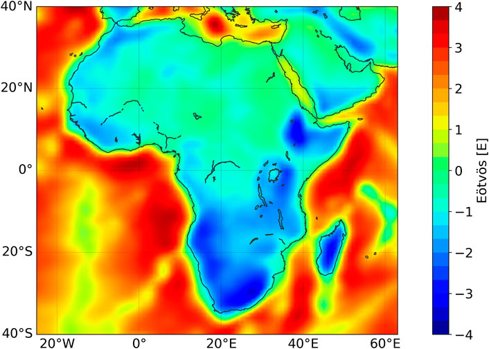
FIGURE 1. Vertical gravity gradient at 225 km height, corrected for topographic and far field isostatic effects. This data set serves as input for the inversion.

When possible, gravity data are corrected for the effect of sediments when applied to inversion for the Moho depth (e.g. Uieda and Barbosa, 2016; Zhao et al., 2020). However, the thickness of a large portion of the African sedimentary basins is unknown. The large uncertainties on lateral and depth extension of the sediment basins make them inappropriate to use as a reliable constraint for correction of the gravity data. In the Supplementary Material we show how the inversion performs with gravity data that has been corrected for the gravitational effect of sediments (Supplementary Figures S1–S6).

2.2 Seismic Data Base

To constrain a gravity-inverted Moho depth additional information on the Moho depth is required, such as a continental data base containing active and/or passive seismic depth estimates (e.g., Uieda and Barbosa, 2016; Haas et al., 2020). Here, we compile a new data base for our study area and decompose it into active (AS) and passive seismic Moho estimates, which are mostly obtained by receiver functions (RF). For the Moho estimates derived by active source seismics we use the data as listed in the USGS Global Seismic Catalogue (Mooney, 2015), which mostly represents reversed refraction data (Szwillus et al., 2019). Additionally, we add active source seismic estimates of the continental data base of Globig et al. (2016). The USGS data base contains data for both the continental and oceanic domains, while the data base of Globig et al. (2016) contains data points over the continent only. For the second data base, we use the continental passive seismic Moho estimates as presented in Globig et al. (2016). We add recent receiver function studies in Namibia (Heit et al., 2015), Botswana (Yu et al., 2015; Fadel et al., 2018), Egypt (Hosny and Nyblade, 2016), Malawi (Sun et al., 2021), and Ethiopia (Wang et al., 2021).

In the next step, each data set is binned on a 1° lateral grid using inverse distance weighting (Figure 2A). This avoids small-scale clusters of seismic stations that may bias the estimated Moho depth and ensures that both gravity and seismic Moho depth are at the same coordinates, superseding a posterior interpolation of the gravity data. We select a search radius of 80 km for the inverse distance weighting. A representative study area in southern Africa shows that 34 receiver functions are removed during the interpolation (Supplementary Figure S7). At the same time, local clusters of different Moho depth estimates are removed, while the general trend of the receiver functions is preserved (Supplementary Figure S7). The final database contains 835 seismic stations, in which both components are almost equally represented (450 AS stations vs. 385 RF stations). For 91 of the stations, AS and RF data give different Moho depth estimates (Figure 2B) with differences up to ±15 km. This discrepancy motivates us to treat active and passive seismic constraints separately when applied to gravity inversion.

FIGURE 2

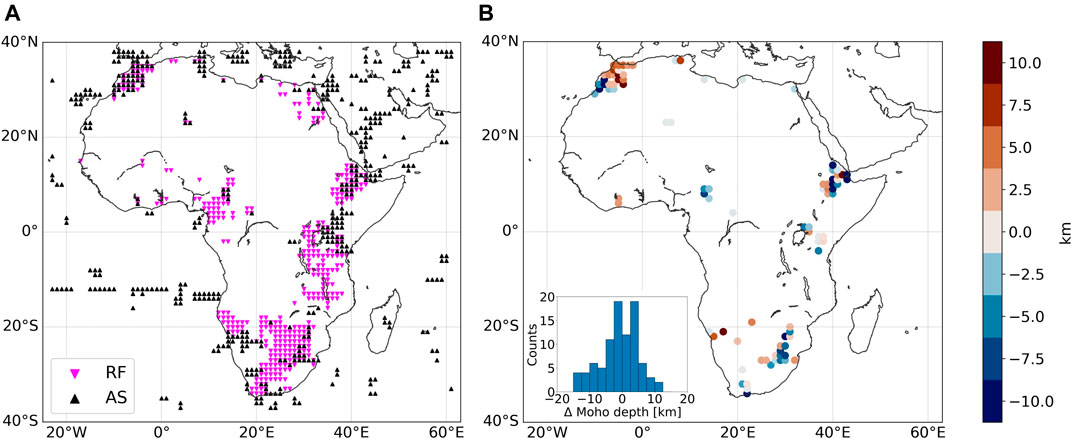
FIGURE 2. Location of the seismic stations, binned on a 1° grid. (A) Active source seismic estimates (AS), marked as black triangles, and receiver functions (RF), marked as pink inverted triangles. (B) Differences of AS and RF estimates at overlapping stations. Red colours indicate deeper RF estimates, blue colours deeper AS estimates. The inset histogram shows the cumulative differences.

2.3 K-Means Clustering of Seismic Tomography

A regionalization map is obtained by clustering seismic tomography data. We applied the k-means algorithm, which is an unsupervised machine learning algorithm. It has been frequently used to cluster seismic tomography data of different scale and resolution (e.g., Lekic and Romanowicz, 2011; Schaeffer and Lebedev, 2015; Garber et al., 2018; Eymold and Jordan, 2019). Compared to other algorithms, it is very fast and efficient. When applied to seismic tomography, it aids in identifying a certain number k of velocity-depth or ‘centroid’ profiles. Each single velocity-depth profile of the tomographic model is then allocated to a cluster in order to minimize the distance to the centroid profile.

The number of clusters k is the parameter that allows a high degree of freedom when clustering data. For a given data set, the number of clusters depends on its size and shape, as well as the target resolution. Lekic and Romanowicz (2011) applied the k-means algorithm to a set of upper mantle tomographies and found that k = 6 clusters “naturally group into families that correspond with known surface tectonics”. Schaeffer and Lebedev (2015) adapted this method to provide a regionalization of their model SL 2013sv, producing six clusters that are translated into different tectonic units.

We tested this approach for the continental seismic tomography model AF2019 of Celli et al. (2020). AF2019 is an azimuthally anisotropic S-wave tomography model for Africa, extending from the crust to the mantle transition zone. In agreement with the parametrization of Schaeffer and Lebedev (2015) we clipped the model AF2019 to 30–350 km, which covers the lower crust and the underlying mantle lithosphere, and sliced the model at 10 km intervals. By using this depth extension, we map distinct tectonic domains that represent the entire lithospheric architecture, rather than internal crustal features. Setting the upper boundary of the model to 30 km additionally ensures that structures of the upper mantle in regions of shallower crust are mapped as well. To be consistent with the measured height of the gravity data and the regularization of the inversion we resampled the model laterally to 1°, which is roughly 100 km (Haas et al., 2020).

We used the elbow method to identify an appropriate number of clusters k for the given data set. Varying the cluster numbers between k = 1 and k = 12, we find no statistical justification for a certain cluster number (Supplementary Figure S8). Instead, k = 6 clusters separate the tomography model in three distinct continental and oceanic tectonic domains that are in accordance with the definition introduced by Schaeffer and Lebedev (2015) (Supplementary Figure S9). Interestingly, the same number of clusters has been independently chosen for models with very different resolution, indicating that the choice of k = 6 reflects distinct seismotectonic units and is not affected by the resolving power of each model. Therefore, we choose k = 6 to represent the seismic tomography in terms of distinct tectonic domains (Figure 3). Compared to the previous regionalizations of Lekic and Romanowicz (2011) and Schaeffer and Lebedev (2015), our new regionalization map shows greater detail in the structure of all three cratons and particularly in the West African and Kalahari Cratons, previously seen as large, uniform blocks, retaining the resolution of AF2019 and validating their robustness across depths.

FIGURE 3

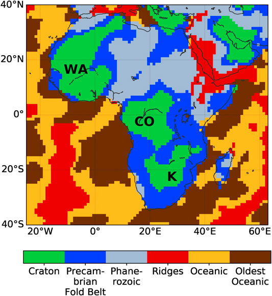
FIGURE 3. Tectonic regionalization map of the AF2019 tomography model. The clusters are translated into distinct tectonic domains, based on the definitions of Lekic and Romanowicz (2011) and Schaeffer and Lebedev (2015). The three continental cratons are indicated as WA=West African Craton, CO=Congo Craton, K=Kalahari Craton.

2.4 Two-step Gravity Inversion

We take the vertical gravity gradient g_zz at 225 km height as initial data to invert for the Moho depth. During the inversion, the density contrast at the Moho depth is kept laterally variable, as defined by the regionalization map. Together with the seismic data base the regionalization map constrains the estimated Moho depth.

We improve this approach by splitting the determination of lateral density variations into two steps. This ensures that closed polygons of the same tectonic domain can be varied individually. From a technical point of view, the imaged cratons of the African continent are well suited to be varied individually, as they form three coherent polygons, keeping the computational effort of the inversion reasonable (Figure 3).

In the first instance, the two hyperparameters, i.e. reference Moho depth z_ref = 32 km and reference density contrast Δ ρ_ref = 400 kg/m³, as well as an initial Moho depth of z₀ = 30 km are used to discretize a tesseroid model. According to Haas et al. (2020) A_ref is obtained by calculating the gravitational effect of shifting z₀ by δz = 1 km. Hence, the dimension of each tesseroid is 1° in lateral direction and 1 km in vertical direction. Using these values, we calculate the Jacobian A_ref only once. A_ref contains the gravitational effect of every g_zz data point (column of matrix) for every tesseroid (row of matrix). In the inversion, we select a range of Δ ρ = 200 : 50: 600 kg/m³, which is in accordance in terms of the compositional change at the Moho depth (Rabbel et al., 2013).

The two-step gravity inversion is based on the selection of tectonic units that are assigned with density contrasts during the inversion. The two steps are as follows:

1. Vary the density contrast for all tectonic units except the cratons (Figure 4A).

2. Vary the density contrast for cratons only (Figure 4B). Each craton is treated separately. Take the preferred density contrasts of step 1 for surrounding tectonic units.

FIGURE 4

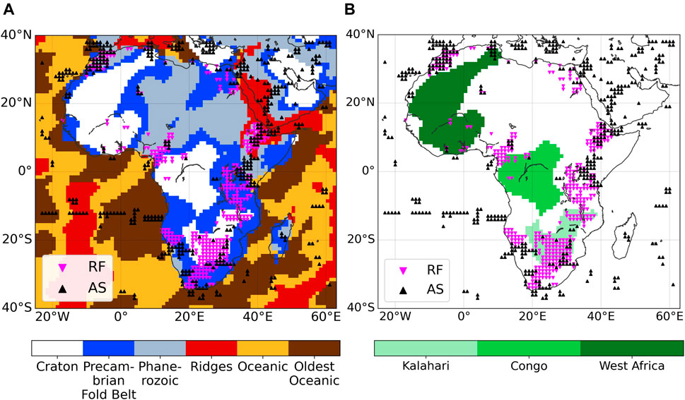
FIGURE 4. Schematic overview on the two steps of the gravity inversion. The triangles indicate the location of AS and RF stations, respectively. (A) Step 1: Vary density contrasts of the units Precambrian, Phanerozoic, Ridges, Oceans, Oldest Oceans. Cratons are masked by white colour. (B) Step 2: Vary density contrasts of individual cratons, namely West African Craton (dark green), Congo Craton (green), Kalahari Craton (light green). Other tectonic units are masked by white colour.

In the first step, nine density contrasts are varied for five tectonic domains, giving a number of n = 9⁵ = 59.049 combinations. For a certain density contrast i the Jacobian is defined as:

$A_i=A_{ref}\frac{\mathrm{\Delta }{\rho }_i}{\mathrm{\Delta }{\rho }_{ref}}(1)$

Where the regionalization defines a craton, Δ ρ_i is set to Δ ρ_ref.

For each iteration i a Moho depth z_i is estimated, derived from the Jacobian A_i (see Eqs. 4–6 in Haas et al., 2020). Together with the seismic estimates z_seis the inverted Moho depth z_i is used to calculate the RMS

$RM{S}_i=\sqrt{\frac{{\sum }_{j=1}^m\left(z_{seis}-z_i\right)}{m}},(2)$

where m is the number of seismic stations. Acknowledging the different station types the RMS is calculated for AS and RF stations separately (RMS_AS and RMS_RF). Afterwards, both RMS values are combined to a single value RMS_i,Comb, weighting the RMS of AS against the RMS of RF:

$RM{S}_{i,Comb}=\frac{RM{S}_{i,AS}\cdot Q+RM{S}_{i,RF}}{Q+1}(3)$

Q defines how much weight is given to the fit of the AS stations. We select Q = 2. This gives double weight to the RMS of the AS stations, as in continental scale data compilations receiver functions of different studies are prone to higher uncertainties (Szwillus et al., 2019). The specific density grid Δ ρ_i, defining the best fitting RMS_i,Comb, is stored for the next step.

In the second step, the density contrast of the three cratonic units are varied, resulting in n = 9³ = 729 combinations. Δ ρ for the other units is taken from the first step. Finally, the density contrasts that define the best-fitting RMS_i,Comb are taken to calculate the final Moho depth.

Splitting the density contrast variations in two steps significantly improves the total number of possible variations from n = 9⁸ = 43.046.721 to n = 9⁵ + 9³ = 59.778 combinations, making this approach computationally very efficient. For details, the reader is referred Haas et al. (2020).

3 Results

Figure 5 shows the density curves for the best-fitting models of both inversion steps, as defined by the combined RMS. The distribution for the individual constraints are documented in the Supplementary Material (Supplementary Figure S10). For the oceanic domains, including ridges, we estimate a density contrast between Δ ρ = 300 − 450 kg/m³ (Figure 5A). The flat curve for ridges is caused by different sensitivities of the constraints (Supplementary Figure S10). For the two continental domains, Precambrian Fold Belts and Phanerozoic, we estimate higher density contrasts. Phanerozoic is expressed as a pronounced maximum at a density contrast of Δ ρ = 600 kg/m³, whereas Precambrian Fold Belts show a rather flat distribution with a preferred density contrast of Δ ρ = 450 kg/m³. For the cratons, the Congo Craton reflects a distinct maximum at Δ ρ = 200 kg/m³, which is the lowest density contrast tested (Figure 5B). Like for the other domains, different sensitivities of AS and RF constraints cause shifts of the individual density curves (Supplementary Figure S10). For the Kalahari Craton, an intermediate density contrast of Δ ρ = 350 kg/m³ is preferred, while the West African Craton shows a smooth distribution of density contrasts with a slight plateau of higher density contrasts (Figure 5B).

FIGURE 5

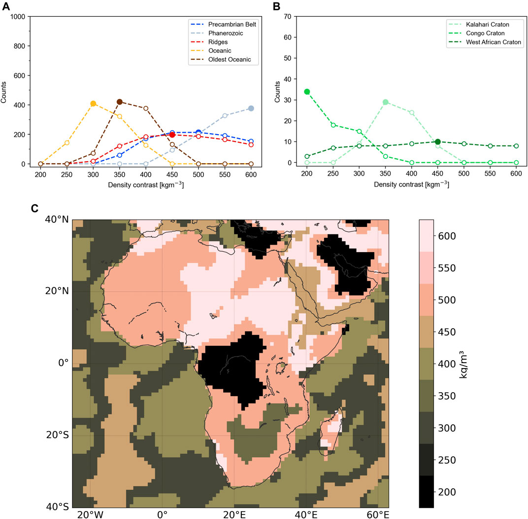
FIGURE 5. (A) Distribution of the density contrasts for the 1,000 best-fitting models of the first inversion step. (B) Distribution of the density contrasts in the second inversion step. Due to a limited number of model solutions only 70 models are compared with each other. Both distributions are shown for the combined RMS of both constraints. (C) Final estimated density contrasts at the Moho depth for the best-fitting model in a gridded space.

In a gridded space, the density contrasts illustrate higher values for continental compared to oceanic domains (Figure 5C). However, for the continents, the range of estimated density contrasts is wider than for the oceans. In the north, the West African Craton is indistinguishable from its surrounding, as the adjacent Precambrian Fold Belts fit the same density contrast (Δ ρ = 450 kg/m³). In the south, the Kalahari Craton slightly contrasts to the surrounding fold belts Δ ρ = 350 kg/m³ vs. Δ ρ = 450 kg/m³). As the most prominent anomaly on the continent, the Congo Craton is clearly distinguished from the Precambrian Fold Belts (Δ ρ = 250 kg/m³ vs. Δ ρ = 450 kg/m³).

The differences of the estimated density contrasts are partly reflected in the corresponding Moho depth (Figure 6A). Offshore, deeper Moho correlates with ridge features like the Walvis Ridge and the Mascarene Plateau in the Indian Ocean. With an average Moho depth of 32.9 km Ridges and Backarks are overestimated in our Moho model (Table 1). There are two reasons for the deep Moho at ridges: First, the gravity data may contain a remnant signal of thermal anomalies in the oceanic lithosphere. For oceanic ridges, this effect is expected to be strongest, as the oceanic lithosphere is very young and hot (Chappell and Kusznir, 2008). Second, parts of the East African Rift System, which is densely covered by seismic stations, fall into the same cluster, causing a bias towards the continents (Figure 4A). For older oceanic lithosphere and deep ocean basins, the Moho depth is mainly shallower than 15 km.

FIGURE 6

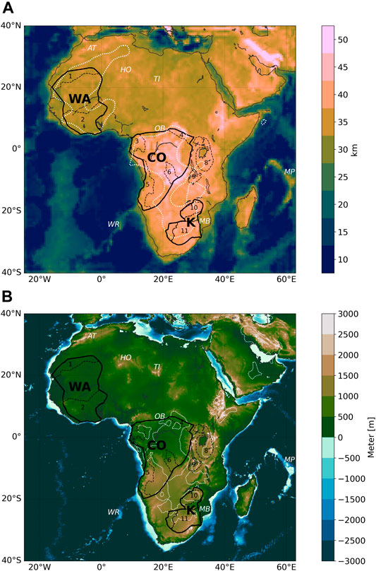
FIGURE 6. (A) Final estimated Moho depth. Black solid contours indicate the extent of the West African Craton (WA), Congo Craton (CO) and Kalahari Craton (K), as seen in surface geology. Black dashed contours represent smaller cratons and individual shields. 1: Reguibat, 2: Man-Leo, 3: Gabon-Cameroon, 4: Bomu-Kibali, 5: Angola, 6: Kasai, 7: Uganda, 8: Tanzania, 9: Bangweulu, 10: Zimbabwe, 11: Kaapvaal. Contours are taken from Begg et al., 2009. Other tectonic domains that are discussed in the text are indicated in white italic letters. AT: Atlas Mountains, HO: Hoggar Mountains, TI: Tibesti Mountains, OB: Oubanguides Mobile Belt, MB: Mozambique Basin, WR: Walvis Ridge, MP: Mascarene Plateau. White dotted lines indicate the +4% dV_s contours between 80–150 km, calculated from the AF2019 model. (B) Topographic map with same contours of cratonic and shield extent as in a). White dotted lines indicate the 40 km contour of the estimated Moho depth of a).

TABLE 1

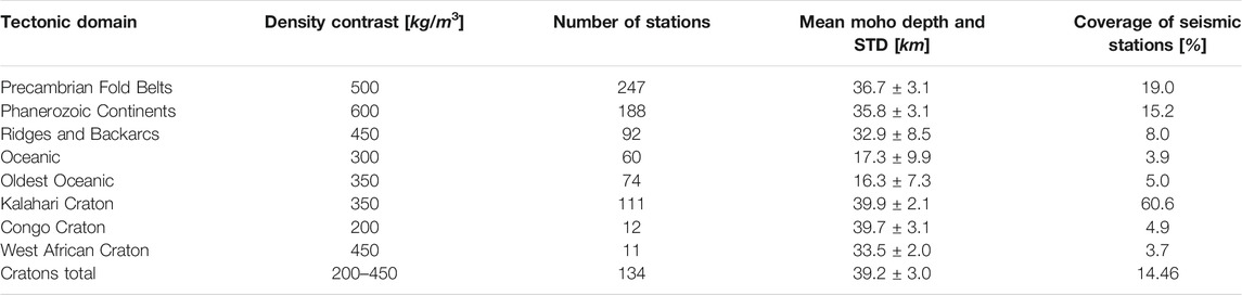
TABLE 1. Estimated density contrasts and distribution of seismic stations. STD = standard deviation.

On the African continent, western and northern Africa are characterized by a rather homogeneous Moho, extending from 30 to 35 km depth. Compared to the oceanic domains the estimated Moho depth is more constant for the individual domains, especially for the cratons, which is expressed by low standard deviation values (Table 1). With an average Moho depth of 33.5 km (Table 1) the West African Craton does not contrast from the surrounding mobile belts. Deeper Moho depths for West and North-East Africa correlate with high topography, including Atlas, Hoggar, and Tibesti Mountains.

As the largest tectonic domain in Central Africa, the Moho of the Congo Craton reaches depths deeper than 50 km in the Kasai Shield, which is the deepest structure of the African continent. However, the average Moho depth is 39.7 km, indicating a Moho with a rather heterogeneous geometry. Towards the northern Oubanguides Mobile Belt the Moho depth displays a sharp contrast. This is well established in the Gabon-Cameroon and Bomu-Kibali Shields, where the Moho depth reveals deep anomalies. In between the two shields and at the eastern boundary, the Moho depth is uplifted to around 35 km.

The adjacent Archean shields to the east (Uganda, Tanzania and Bangweulu) are characterized by an intermediate continental Moho depth around 40 km. In the Afar region further north, the Moho depth reaches up to 50 km.

The deep Moho of the Congo Craton extends through the Proterozoic fold belts inside the Kalahari Craton, which has an average Moho depth of 39.9 km (Table 1). The Moho depth for the internal Archean sub-cratons (Kaapvaal and Zimbabwe) is similar. This gives a homogeneous Moho depth of the Kalahari Craton, as expressed by a low standard deviation of 2.1 km (Table 1). Only the eastern boundary coincides with a sharp contrast in the Moho depth. Here, the Moho depth changes from 40 km in the Kalahari Craton to less than 30 km in the Mesozoic Mozambique Basin.

In many regions, the deep Moho depth correlates with high topography, i.e., in the East African Rift System, Tanzania Craton, Bangweulu Block, and parts of the Kalahari Craton (Figure 6B). In the southwestern Congo Craton, the high topography of the Angolan Shield partly correlates with a deep Moho. Towards the northern part of the Congo Craton, topography decreases to less than 500 m, while the deeper Moho is maintained to a large extent.

Our models for the Moho depth and associated density contrasts are estimated by the best-fitting Moho model compared to the initial seismic stations. Figure 7 shows the fit to the seismic stations for AS and RF constraints separately. For the AS constraints, the estimated Moho depth is more than 10 km deeper in the East African Rift System and the Cameroon Volcanic Line (Figure 7A). The latter is constrained by five stations north of the Congo Craton. West of the Kalahari Craton several station clusters reveal Moho depth estimates more than 10 km shallower. Locally, the differences between Moho depth estimates and AS constraints can be higher than 20 km (Figure 7C). However, most stations are binned between ±10 km. With a mean value of 1.51 km the estimated Moho depth is slightly deeper than the AS constraints.

FIGURE 7

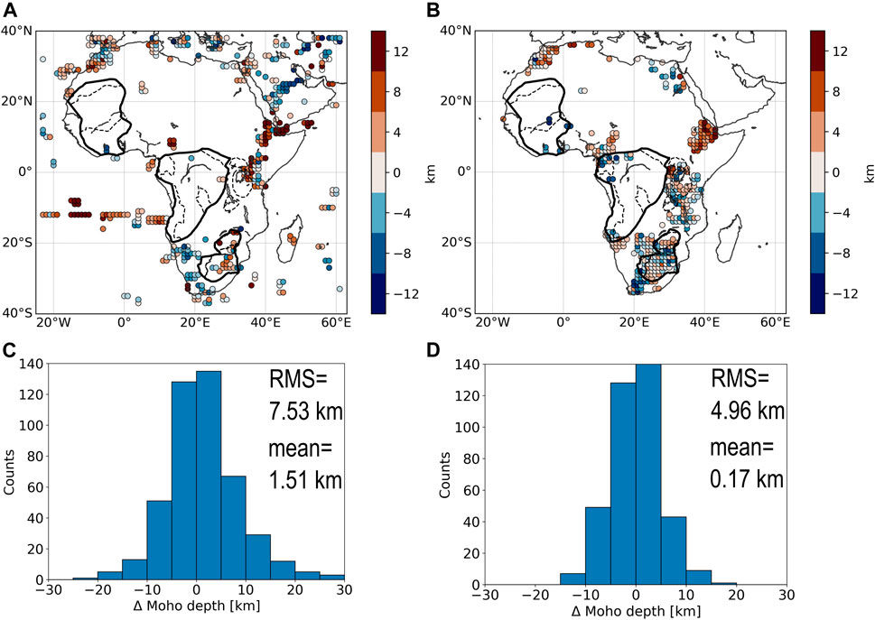
FIGURE 7. Fit of the estimated Moho depth to the seismic constraints. Red colours indicate a deeper estimated Moho depth, while blue colours indicate a shallower Moho depth compared to the seismic constraints. (A) Estimated Moho depth minus AS constraints, (B) Estimated Moho depth minus RF constraints, (C) Histogram of differences for AS constraints, (D) Histogram of differences for RF constraints.

For the RF constraints, the estimated Moho depth of the East African Rift System is deeper as well (Figure 7B), even though the difference is less strong as for the AS constraints. The well covered Kalahari Craton, as well as the Tanzania and Uganda Shield show a good fit with differences mainly within ±4 km. In the area of the Gabon-Cameroon Shield the estimated Moho depth is locally more than 12 km shallower. To the north, in the adjacent Cameroon Volcanic Line, this trend changes and the Moho depth estimate is only up to 4 km deeper than the RF constraints.

Interestingly, the cumulative histogram shows a better fit for the RF estimates compared to the AS estimates (Figure 7D), which is also expressed in the RMS_RF value (4.96 km RF vs 7.53 km for AS). There are two reasons for the better fit of the RF estimates: First, offshore stations lack in the RF data base. As a consequence, the overestimated Moho depth for ridges are not reflected in the RMS. Second, more RF than AS estimates are available for the continent, resulting in a good match of RF estimates with the gravity-estimated Moho for large parts of the Kalahari, Tanzania, and Uganda Cratons.

4 Discussion

4.1 Limitations of the Estimated Density Contrasts

The significance of the estimated density contrasts for each tectonic domain is manifested in the peaks of the density curves (Figure 5). Haas et al. (2020) showed that station coverage and amplitude of the gravity signal control the estimated density contrast distributions. This observation is also valid for the African continent, even though the poor station coverage in some tectonic domains hampers a progressive increase of density contrasts with tectonic age, as observed in the Amazonian Craton and its surroundings (Haas et al., 2020). The estimated density contrasts for the Phanerozoic domain and for the Congo Craton are located at the boundaries of the given range, representing realistic petrological assumptions (see Data and Methods). Nevertheless, the trend of the estimated density contrasts shows a flattening of the curve for the Phanerozoic domain, indicating that the estimated density contrasts are close to the theoretical peak. For the Congo Craton, the curve represents the dependence of the estimated density contrasts to a low number of receiver functions.

For the Phanerozoic domain, the seismic stations are predominantly located in mountainous regions (Atlas, Great Rift Valley, and Cameroon Volcanic Line), which are characterized by a deeper Moho that isostatically compensates the high topography. This coincides with a high density contrast across the Moho, which is also confirmed by gravity inversions in mountain ranges (e.g., Zhao et al., 2020). In the East African Rift System, the Moho depth is overestimated compared to both seismic constraints because of an unaccounted gravity signal of the upwelling mantle. Contrary to this, for the Cameroon Volcanic Line the AS constraints show a worse fit to the estimated Moho depth compared to the RF constraints of Tokam et al. (2010). However, in the same study, a deeper Moho depth between 43–48 km for the northern Congo Craton is identified, which is in stark contrast to our estimated Moho depth.

The impact of the poor station coverage is highly evident in the cratonic units. For the Congo Craton, the density curve of the AS constraints is flat, because no constraints are located in the Congo Craton (Supplementary Figure S10 and Table 1). Here, only few receiver functions that are located in the vicinity of the Congo Basin (Tokam et al., 2010) can be used to make any assumptions on Moho depth and density contrast. Given the sparse distribution of seismic stations and the uncertainties of sediment thickness, the Congo Craton contrasts to the surrounding fold belts by a distinct low density contrast, which fits in the classical view of smooth density transitions in cratonic lithosphere. However, the impact of the available sediment data on the estimated Moho depth illustrates that it is almost impossible to predict the Moho depth precisely. Clearly, more seismic stations are required to shed light in the crustal architecture of the Congo Basin and Congo Craton.

The West African Craton reflects the smoothest density curve of all cratons, which is caused both by the lowest station coverage of all tectonic units and the low amplitude of the gravity data (Table 1 and Figure 1). Generally, a low gravity signal inherently implies a flat Moho geometry. That means, even if the West African Craton was densely covered by seismic stations, the estimated Moho depth would not change significantly. Coincidentally, a wide range of density contrasts can explain the observed gravity signal, like it is the case for the West African Craton.

The large Moho depth variations between gravity and receiver functions estimates on a small scale illustrate the limits of the constraining procedure. Velocity contrasts do not necessarily coincide with density contrasts, especially between different tectonic settings, and variations in temperature and anisotropy can affect the local velocity structure (e.g., Fullea et al., 2021). To overcome this discrepancy a more detailed analysis on combining the characteristics of both methods is required. One strategy forward would be to calculate synthetic receiver functions from the initial density model, using published density to velocity conversions (e.g. Julià, 2007; Masters et al., 2011).

4.2 Comparison With Other Moho Depth Models

In this section, we compare our estimated Moho depth model on continental scale with the continental model of Globig et al. (2016) (Globig-Moho) and the global model of Szwillus et al. (2019) (Szwillus-Moho). The Globig-Moho represents the latest continental Moho model, while the Szwillus-Moho is a global Moho model, obtained by interpolation of active source seismics only. It is derived by the USGS GSC data base that serves as pointwise constraint in our inversion. Therefore, a comparison with the Szwillus-Moho reflects the difference to the seismic Moho depth in a gridded space.

Like our estimated Moho depth model the Globig-Moho shows a deeper Moho for central and southern Africa, including the Congo and Kalahari Cratons (Figure 8A). However, the bimodal pattern is not as pronounced as in our model. In the Globig-Moho, the West African Craton progressively thickens towards the Atlas Mountains and thins towards the West African coast. In our model, the Moho of the West African Craton is mainly flat. The difference map shows a long-wavelength trend that documents the upper mantle contribution in the geoid anomaly map that Globig et al. (2016) used as input data (Figure 8C). Similar to our model, the Globig-Moho in the Afar region is characterized by a deep Moho. The deep Moho depth of both models represent isostatic compensation caused by high topography. This is also reflected in the gravity data (Figure 1). The question is then how representative the isostatic state is for the Afar region. As the Afar region is underlain by an active plume, isostasy might be an inappropriate representation of the lithospheric state (Czechowski, 2019). Our Moho model rather shows the hypothetic isostatic state caused by the elevated topography in the Afar region.

FIGURE 8

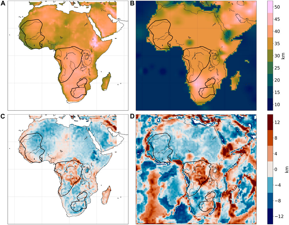
FIGURE 8. Comparison of Moho depth models. (A) Moho depth model of Globig et al. (2016), which is only defined for the African continent. (B) Moho depth model of Szwillus et al. (2019). (C) Difference of our estimated Moho model minus Globig-Moho. (D) Difference of our estimated Moho model minus Szwillus-Moho. Contours indicate cratons and shields, taken from Figure 6.

The Szwillus-Moho predominantly displays long-wavelength structures that arise from the sparse coverage of seismic stations (Figure 8B). As in all data-sparse regions, like the West African and Congo Cratons, the Szwillus-Moho represents global mean values for continental Moho depth. Therefore, these two cratons cannot be differentiated. The only region where the Moho depth varies on small scale is the East African Rift System. Here, the Moho depth deepens from 20 km in the Afar Region to 45 km in the Ethiopian Highlands and back to 25 km in the Great Rift Valley of Ethiopia. In our model, this region is characterized by a Moho more than 12 km deeper than the Szwillus-Moho (Figure 8D). Most probably, the differences reflect an unaccounted gravity signal of the underlying Afar plume.

The general difference pattern reflects stronger amplitudes compared to the Globig-Moho. A shallower Moho is located in the East African System and Congo Craton, as well as in the southern Kalahari Craton, whereas deeper Moho can be found in the Mozambique Basin and Damara Belt, separating the Congo Craton from the Kalahari Craton. The comparison to the Szwillus-Moho reproduces the difference of the pointwise constraints (Figure 7A), as well as the difference to average continental Moho depth in data sparse regions in a gridded space.

4.3 Correlation Between Archean Crust and Archean Lithospheric Mantle

The general architecture of mid-Archean lithosphere is characterized by thick lithosphere and a shallow and sharp Moho (Artemieva, 2009; Abbott et al., 2013). In Paleoproterozoic regions, the crust gradually thickens and the Moho gets more diffuse in terms of v_p/v_s-ratios (Abbott et al., 2013; Yuan, 2015). The West Australian Craton can be regarded as a classic example that fulfills those criteria (Yuan, 2015). However, cratonic regions like the West African Craton might not fit in this uniform picture. In what follows, we investigate how the three African cratons fit in this uniform picture and link the gravity-derived Moho depth to the geographic extension of cratons, as imaged by seismic tomography (Celli et al., 2020).

Cratonic lithosphere can be affected by various mechanisms. On the one hand, the composition and temperature of cratonic mantle lithosphere can be modified by metasomatism and plume activity (e.g., Lee et al., 2011; Kusky et al., 2014; Dave and Li, 2016; Wenker and Beaumont, 2018). On the other hand, its thermal boundary layer can be mechanically eroded or recycled into the convective mantle. In addition, it is often proposed that in the Archean the denser lower crust was delaminated and recycled into the convective mantle, therefore before cratonization (Abbott et al., 2013). Using seismic tomography, bedrock geology, and diamondiferous kimberlites, Celli et al. (2020) showed that a large portion of the African cratons has been eroded by mantle plumes.

The lateral extension of the Congo and Kalahari Cratons coincides with a Moho deeper than 40 km (Figure 6A). This could suggest late-to post-Archean crustal thickening before stabilization of the crust. However, the stabilization of the Kalahari Craton is dated to mid-Archean (Abbott et al., 2013 and references within). For the Kalahari Craton, magmatic underplating triggered by the Karoo volcanism might be an alternative explanation for the deep crust (Cox, 1993). However, 3D modelling suggests that the high topography is largely isostatically compensated by the crust, accompanied by lateral changes in lithospheric mantle density (Scheiber-Enslin et al., 2016). In this study, only a small portion of the topographic signal is explained by buoyant asthenosphere, causing excess elevation of the African superswell (Lithgow-Bertelloni and Silver, 1998). We follow the study of Scheiber-Enslin et al. (2016) and interpret the deep Moho depth of the Kalahari Craton as isostatic compensation of high topography. The same mechanism might explain the deep Moho for the Congo Craton, even though missing data of stabilization age and Neoproterozoic subsidence of the Congo Basin are additional sources that need to be considered. Located in the center of the Congo Craton, the lighter sediments of the Congo Basin may uplift the Moho depth a few kilometers. However, the overall pattern of deeper Moho depth is preserved (Supplementary Figure S4). Furthermore, large uncertainties in the sedimentary data base hamper a valid assessment of the gravitational effect.

Some Archean shields are not imaged by seismic tomography (Figure 6). This is evident for the Angolan Shield, as well as the Uganda and Tanzania Cratons. Celli et al. (2020) propose that the missing cratonic root for the Angolan Shield is the result of Tristan Plume activity, and for the Tanzania and Uganda Cratons by ongoing activity of the Afar Plume. Our estimated Moho depth shows that Archean crust is still preserved, while the underlying lithosphere has been partially eroded, indicating that the crustal structure has been affected only little by the process of cratonic destruction. At the southeastern edge of the Angolan Shield, the deep Moho partly correlates with high topography (Figure 6B). This small scale topographic uplift ocurred in the Neogene, forming the so called Angola dome (Klöcking et al., 2020). The uplift of the Angola dome might be sourced from a small positive temperature anomaly in the asthenosphere, causing thinning of the overlying mantle (Klöcking et al., 2020), while the deep Moho has been preserved (Figure 6A). Such a rejuvenation of the lithospheric mantle has also been observed for other cratons like the Wyoming Craton and the North China Craton (Gao et al., 2004; Zhao et al., 2009; Dave and Li, 2016).

The West African Craton is in stark contrast to the other African cratons. While seismic tomography reveals a large lateral extension of cratonic lithosphere, the Moho depth is shallow and does not differentiate from the surrounding tectonic units. The sediments of the Neoproterozoic Taoudeni Basin contribute only minor the estimated Moho depth (Supplementary Figures S4, S5). As the West African Craton amalgamated in the Paleoproterozoic (e.g., Block et al., 2015), the Moho depth is expected to be deeper than older cratons (Abbott et al., 2013). This raises the following question: Which process (es) caused the thinning of the crust without affecting the lithosphere?

Analysis of geological and geochronological data from NW Ghana suggests that the lower crust was largely exhumed and juxtaposed against the shallow crust during the Eburnean orogeny (2.15–2.0 Ga, Block et al., 2015). This exhumation involves extensional detachments that stretch and thin the upper crust, providing the space in the upper crust for the lower crust to flow into. The horizontal flow of the weak lower crust from regions of thicker crust towards regions of thinner crust would result in a thinner continental crust and a flat and shallower Moho. However, this process of gravitational collapse is often driven by to the convective removal of the thermal boundary layer of the lithosphere, which leads to thinning of the entire lithosphere (Rey et al., 2001; Rey et al., 2017). The preserved buoyancy of the Archean keel at the time of the Eburnean Orogeny may have prevented the recycling of the lithosphere thermal boundary layer into the convective mantle. Nevertheless, the association of a thinned crust, with a preserved thick lithospheric root remains enigmatic.

5 Conclusion

We have investigated the variable lithospheric architecture of the African cratons, based on a new gravity-derived continental Moho depth model. The model is constrained by a state-of-the-art tectonic regionalization map, calculated from the AF 2019 tomography model, and an updated seismic data base. This data base comprises different acquisition types that we distinguish between active source seismics and receiver functions.

Our two-step gravity inversion updates the method of Haas et al. (2020) by allowing flexible density contrasts for individual tectonic units. This splitting in two steps strongly decreases computation time. The estimated density contrasts at the Moho reveal large differences between the different tectonic domains and between the individual cratons. For the Congo Craton, we identify a density contrast of Δ ρ = 200 kg/m³. The Kalahari Craton is the best-constrained tectonic unit and shows an intermediate density contrast of Δ ρ = 350 kg/m³, which is typical of what we expect between the lower continental crust and the mantle. Uncertainties in the estimated density contrasts arise from different measuring techniques and sparse data coverage. This is well reflected in the poor distribution of density curves for the West African Craton.

The estimated Moho depth shows a bimodal pattern with deeper crust for the Congo and Kalahari Cratons and shallower crust for the West African Craton. The sediments of the intracratonic Congo and Taoudeni Basins, whose architecture is largely unknown, do not significantly change this observed pattern. We have demonstrated that the differences between the estimated Moho depth and the seismic constraints are not necessarily constant for both constraint types. This is well reflected in the Cameroon Volcanic Line, where the estimated Moho depth model fits receiver function constraints better than those from active source seismics.

We have analyzed the coupling between our Moho depth model and high seismic velocities in the mantle, as imaged by seismic tomography for the cratonic regions. For the southern and central cratons, the lithospheric keel matches with a deep Moho depth. Here, the deep Moho depth more likely represents an isostatic root of elevated topography and thick Archean crust. Contrary to that, the deep lithosphere of the West African Craton coincides with a flat and homogeneous Moho depth. Lower crustal exhumation with subsequent crustal flow and gravitational collapse cannot explain the observed pattern. Thus, for the West African Craton the observed lithospheric architecture remains enigmatic.

Clearly, more data from both active and seismic methods is required to further investigate the lithosphere of the West African and Congo Cratons. This would also help to disentangle the role of the yet very poorly explored big intracratonic sedimentary Congo and Taoudeni Basins for cratonic evolution.

In a next step, the variable build-up of the cratonic portions, as seen by the joint gravity inversion and seismological regionalization approach, should be tested for another continent. Moho depth variations between gravity and receiver functions estimates could be further investigated by calculating synthetic receiver functions from the accompanying density model. Special focus should be put to the coupling of the crustal and lithospheric structure, which is crucial for understanding the cratonization and destabilization of Earth’s early crust.

Data Availability Statement

Gravity gradient data are available from ESA: https://earth.esa.int/eogateway/missions/goce/goce-gravity-gradients-grids. The seismic tomography model AF2019 can be downloaded from the following webpage: https://nlscelli.wixsite.com/ncseismology/models. The constraints of seismic Moho depth are taken from the Globig et al. (2016) paper: https://agupubs.onlinelibrary.wiley.com/doi/full/10.100 2/2 016JB012972. Our estimated Moho depths, both with and without sediments, as well as the estimated density contrasts are available on the Github link below. We encourage the scientific community to test the presented inversion for their purposes. Therefore, we share our code on Github, where the inversion is reconstructed for a smaller test area: https://github.com/peterH105/Gradient_Inversion/.

Author Contributions

All authors listed have made a substantial, direct, and intellectual contribution to the work and approved it for publication.

Funding

This work has been funded by the Deutsche Forschungsgemeinschaft (DFG) within the project “Linking the deep structures of the cratons of Africa and South America by integrated geophysical modelling” (project number 336717379), as well as by European Space Agency (ESA) as a Support to Science Element (STSE) within the project “3D Earth-A Dynamic Living Planet.”

Acknowledgments

We thank Wolfgang Szwillus for discussions on clustering of seismic tomography data and implementing the gravity inversion code. All figures have been created with Matplotlib. We are thankful for the valuable comments of three reviewers.

Conflict of Interest

The authors declare that the research was conducted in the absence of any commercial or financial relationships that could be construed as a potential conflict of interest.

The handling editor declared a past collaboration with one of the authors JE.

Publisher’s Note

All claims expressed in this article are solely those of the authors and do not necessarily represent those of their affiliated organizations, or those of the publisher, the editors and the reviewers. Any product that may be evaluated in this article, or claim that may be made by its manufacturer, is not guaranteed or endorsed by the publisher.

Supplementary Material

The Supplementary Material for this article can be found online at: https://www.frontiersin.org/articles/10.3389/feart.2021.696674/full#supplementary-material

References

Abbott, D. H., Mooney, W. D., and VanTongeren, J. A. (2013). The Character of the Moho and Lower Crust within Archean Cratons and the Tectonic Implications. Tectonophysics 609, 690–705. doi:10.1016/j.tecto.2013.09.014

CrossRef Full Text | Google Scholar

Artemieva, I. M. (2009). The continental Lithosphere: Reconciling thermal, Seismic, and Petrologic Data. Lithos 109, 23–46. doi:10.1016/j.lithos.2008.09.015

CrossRef Full Text | Google Scholar

Artemieva, I. M., and Vinnik, L. P. (2016). Density Structure of the Cratonic Mantle in Southern Africa: 1. Implications for Dynamic Topography. Gondwana Res. 39, 204–216. doi:10.1016/j.gr.2016.03.002

CrossRef Full Text | Google Scholar

Begg, G. C., Griffin, W. L., Natapov, L. M., O'Reilly, S. Y., Grand, S. P., O'Neill, C. J., et al. (2009). The Lithospheric Architecture of Africa: Seismic Tomography, Mantle Petrology, and Tectonic Evolution. Geosphere 5, 23–50. doi:10.1130/GES00179.1

CrossRef Full Text | Google Scholar

Block, S., Ganne, J., Baratoux, L., Zeh, A., Parra-Avila, L. A., Jessell, M., et al. (2015). Petrological and Geochronological Constraints on Lower Crust Exhumation during Paleoproterozoic (Eburnean) Orogeny, NW Ghana, West African Craton. J. Meta. Geol. 33, 463–494. doi:10.1111/jmg.12129

CrossRef Full Text | Google Scholar

Bouman, J., Ebbing, J., Fuchs, M., Sebera, J., Lieb, V., Szwillus, W., et al. (2016). Satellite Gravity Gradient Grids for Geophysics. Sci. Rep. 6, 21050. doi:10.1038/srep21050

PubMed Abstract | CrossRef Full Text | Google Scholar

Celli, N. L., Lebedev, S., Schaeffer, A. J., and Gaina, C. (2020). African Cratonic Lithosphere Carved by Mantle Plumes. Nat. Commun. 11, 92. doi:10.1038/s41467-019-13871-2

PubMed Abstract | CrossRef Full Text | Google Scholar

Chappell, A. R., and Kusznir, N. J. (2008). Three-dimensional Gravity Inversion for Moho Depth at Rifted continental Margins Incorporating a Lithosphere thermal Gravity Anomaly Correction. Geophys. J. Int. 174, 1–13. doi:10.1111/j.1365-246X.2008.03803.x

CrossRef Full Text | Google Scholar

Cox, K. G. (1993). Continental Magmatic Underplating. Phil. Trans. R. Soc. Lond. A. 342, 155–166. doi:10.1098/rsta.1993.0011

CrossRef Full Text | Google Scholar

Czechowski, L. (2019). Mantle Flow and Determining Position of LAB Assuming Isostasy. Pure Appl. Geophys. 176, 2451–2463. doi:10.1007/s00024-019-02093-8

CrossRef Full Text | Google Scholar

Dave, R., and Li, A. (2016). Destruction of the Wyoming Craton: Seismic Evidence and Geodynamic Processes. Geology 44, 883–886. doi:10.1130/G38147.1

CrossRef Full Text | Google Scholar

Doucouré, C. M., and de Wit, M. J. (2003). Old Inherited Origin for the Present Near-Bimodal Topography of Africa. J. Afr. Earth Sci. 36, 371–388. doi:10.1016/S0899-5362(03)00019-8

CrossRef Full Text | Google Scholar

Emry, E. L., Shen, Y., Nyblade, A. A., Flinders, A., and Bao, X. (2019). Upper Mantle Earth Structure in Africa from Full‐Wave Ambient Noise Tomography. Geochem. Geophys. Geosyst. 20, 120–147. doi:10.1029/2018GC007804

CrossRef Full Text | Google Scholar

Eymold, W. K., and Jordan, T. H. (2019). Tectonic Regionalization of the Southern California Crust from Tomographic Cluster Analysis. J. Geophys. Res. Solid Earth 124, 11840–11865. doi:10.1029/2019JB018423

CrossRef Full Text | Google Scholar

Fadel, I., van der Meijde, M., and Paulssen, H. (2018). Crustal Structure and Dynamics of Botswana. J. Geophys. Res. Solid Earth 123 (10659–10), 10659–10671. doi:10.1029/2018JB016190

CrossRef Full Text | Google Scholar

Fishwick, S., and Bastow, I. D. (2011). Towards a Better Understanding of African Topography: A Review of Passive-Source Seismic Studies of the African Crust and Upper Mantle. Geol. Soc. Lond. Spec. Publications 357, 343–371. doi:10.1144/SP357.19

CrossRef Full Text | Google Scholar

Fishwick, S. (2010). Surface Wave Tomography: Imaging of the Lithosphere-Asthenosphere Boundary beneath central and Southern Africa? Lithos 120, 63–73. doi:10.1016/j.lithos.2010.05.011

CrossRef Full Text | Google Scholar

François, T., Burov, E., Meyer, B., and Agard, P. (2013). Surface Topography as Key Constraint on Thermo-Rheological Structure of Stable Cratons. Tectonophysics 602, 106–123. doi:10.1016/j.tecto.2012.10.009

CrossRef Full Text | Google Scholar

Fullea, J., Lebedev, S., Martinec, Z., and Celli, N. L. (2021). WINTERC-G: Mapping the Upper Mantle Thermochemical Heterogeneity from Coupled Geophysical-Petrological Inversion of Seismic Waveforms, Heat Flow, Surface Elevation and Gravity Satellite Data. Geophys. J. Int. 226, 146–191. doi:10.1093/gji/ggab094

CrossRef Full Text | Google Scholar

Gao, S., Rudnick, R. L., Yuan, H.-L., Liu, X.-M., Liu, Y.-S., Xu, W.-L., et al. (2004). Recycling Lower continental Crust in the North China Craton. Nature 432, 892–897. doi:10.1038/nature03162

PubMed Abstract | CrossRef Full Text | Google Scholar

Garber, J. M., Maurya, S., Hernandez, J. A., Duncan, M. S., Zeng, L., Zhang, H. L., et al. (2018). Multidisciplinary Constraints on the Abundance of diamond and Eclogite in the Cratonic Lithosphere. Geochem. Geophys. Geosyst. 19, 2062–2086. doi:10.1029/2018GC007534

CrossRef Full Text | Google Scholar

Globig, J., Fernàndez, M., Torne, M., Vergés, J., Robert, A., and Faccenna, C. (2016). New Insights into the Crust and Lithospheric Mantle Structure of Africa from Elevation, Geoid, and thermal Analysis. J. Geophys. Res. Solid Earth 121, 5389–5424. doi:10.1002/2016JB012972

CrossRef Full Text | Google Scholar

Haas, P., Ebbing, J., and Szwillus, W. (2020). Sensitivity Analysis of Gravity Gradient Inversion of the Moho Depth-A Case Example for the Amazonian Craton. Geophys. J. Int. 221, 1896–1912. doi:10.1093/gji/ggaa122

CrossRef Full Text | Google Scholar

Heit, B., Yuan, X., Weber, M., Geissler, W., Jokat, W., Lushetile, B., et al. (2015). Crustal Thickness and Vp/Vs Ratio in NW Namibia from Receiver Functions: Evidence for Magmatic Underplating Due to Mantle Plume-Crust Interaction. Geophys. Res. Lett. 42, 3330–3337. doi:10.1002/2015GL063704

CrossRef Full Text | Google Scholar

Hosny, A., and Nyblade, A. (2016). The Crustal Structure of Egypt and the Northern Red Sea Region. Tectonophysics 687, 257–267. doi:10.1016/j.tecto.2016.06.003

CrossRef Full Text | Google Scholar

Hu, J., Liu, L., Faccenda, M., Zhou, Q., Fischer, K. M., Marshak, S., et al. (2018). Modification of the Western Gondwana Craton by Plume-Lithosphere Interaction. Nat. Geosci 11, 203–210. doi:10.1038/s41561-018-0064-1

CrossRef Full Text | Google Scholar

Jessell, M. W., Begg, G. C., and Miller, M. S. (2016). The Geophysical Signatures of the West African Craton. Precambrian Res. 274, 3–24. doi:10.1016/j.precamres.2015.08.010

CrossRef Full Text | Google Scholar

Julià, J. (2007). Constraining Velocity and Density Contrasts across the Crust-Mantle Boundary with Receiver Function Amplitudes. Geophys. J. Int. 171, 286–301. doi:10.1111/j.1365-2966.2007.03502.x

CrossRef Full Text | Google Scholar

Klöcking, M., Hoggard, M. J., Rodríguez Tribaldos, V., Richards, F. D., Guimarães, A. R., Maclennan, J., et al. (2020). A Tale of Two Domes: Neogene to Recent Volcanism and Dynamic Uplift of Northeast Brazil and Southwest Africa. Earth Planet. Sci. Lett. 547, 116464. doi:10.1016/j.epsl.2020.116464

CrossRef Full Text | Google Scholar

Kusky, T. M., Windley, B. F., Wang, L., Wang, Z., Li, X., and Zhu, P. (2014). Flat Slab Subduction, Trench Suction, and Craton Destruction: Comparison of the North China, Wyoming, and Brazilian Cratons. Tectonophysics 630, 208–221. doi:10.1016/j.tecto.2014.05.028

CrossRef Full Text | Google Scholar

Lebedev, S., Boonen, J., and Trampert, J. (2009). Seismic Structure of Precambrian Lithosphere: New Constraints from Broad-Band Surface-Wave Dispersion. Lithos 109, 96–111. doi:10.1016/j.lithos.2008.06.010

CrossRef Full Text | Google Scholar

Lee, C.-T. A., Luffi, P., and Chin, E. J. (2011). Building and Destroying continental Mantle. Annu. Rev. Earth Planet. Sci. 39, 59–90. doi:10.1146/annurev-earth-040610-133505

CrossRef Full Text | Google Scholar

Lekic, V., and Romanowicz, B. (2011). Tectonic Regionalization without A Priori Information: A Cluster Analysis of Upper Mantle Tomography. Earth Planet. Sci. Lett. 308, 151–160. doi:10.1016/j.epsl.2011.05.050

CrossRef Full Text | Google Scholar

Lithgow-Bertelloni, C., and Silver, P. G. (1998). Dynamic Topography, Plate Driving Forces and the African Superswell. Nature 395, 269–272. doi:10.1038/26212

CrossRef Full Text | Google Scholar

Masters, G., Woodhouse, J. H., and Freeman, G. (2011). Mineos v1.0.2 [software], Computational Infrastructure for Geodynamics. Available at: https://geodynamics.org/cig/software/mineos/.

Google Scholar

Mooney, W. D. (2015). “Crust and Lithospheric Structure – Global Crustal Structure,” in Treatise on Geophysics. Editor G. Schubert (Amsterdam: Elsevier), 361–398.

Google Scholar

Rabbel, W., Kaban, M., and Tesauro, M. (2013). Contrasts of Seismic Velocity, Density and Strength across the Moho. Tectonophysics 609, 437–455. doi:10.1016/j.tecto.2013.06.020

CrossRef Full Text | Google Scholar

Rey, P. F., Mondy, L., Duclaux, G., Teyssier, C., Whitney, D. L., Bocher, M., et al. (2017). The Origin of Contractional Structures in Extensional Gneiss Domes. Geology 45, 263–266. doi:10.1130/G38595.1

CrossRef Full Text | Google Scholar

Rey, P., Vanderhaeghe, O., and Teyssier, C. (2001). Gravitational Collapse of the continental Crust: Definition, Regimes and Modes. Tectonophysics 342, 435–449. doi:10.1016/S0040-1951(01)00174-3

CrossRef Full Text | Google Scholar

Schaeffer, A. J., and Lebedev, S. (2015). “Global Heterogeneity of the Lithosphere and Underlying Mantle: A Seismological Appraisal Based on Multimode Surface-Wave Dispersion Analysis, Shear-Velocity Tomography, and Tectonic Regionalization,” in The Earth’s Heterogeneous Mantle. Editors A. Khan, and F. Deschamps (Cham: Springer International Publishing), 3–46. doi:10.1007/978-3-319-15627-9_1

CrossRef Full Text | Google Scholar

Scheiber-Enslin, S. E., Ebbing, J., and Webb, S. J. (2016). An Isostatic Study of the Karoo basin and Underlying Lithosphere in 3-d. Geophys. J. Int. 206, 774–791. doi:10.1093/gji/ggw164

CrossRef Full Text | Google Scholar

Sobh, M., Ebbing, J., Mansi, A. H., Götze, H. J., Emry, E. L., and Abdelsalam, M. G. (2020). The Lithospheric Structure of the Saharan Metacraton from 3‐D Integrated Geophysical‐Petrological Modeling. J. Geophys. Res. Solid Earth 125, 2511. doi:10.1029/2019JB018747

CrossRef Full Text | Google Scholar

Sun, M., Gao, S. S., Liu, K. H., Mickus, K., Fu, X., and Yu, Y. (2021). Receiver Function Investigation of Crustal Structure in the Malawi and Luangwa Rift Zones and Adjacent Areas. Gondwana Res. 89, 168–176. doi:10.1016/j.gr.2020.08.015

CrossRef Full Text | Google Scholar

Szwillus, W., Afonso, J. C., Ebbing, J., and Mooney, W. D. (2019). Global Crustal Thickness and Velocity Structure from Geostatistical Analysis of Seismic Data. J. Geophys. Res. Solid Earth 124, 1626–1652. doi:10.1029/2018JB016593

CrossRef Full Text | Google Scholar

Szwillus, W., Ebbing, J., and Holzrichter, N. (2016). Importance of Far-Field Topographic and Isostatic Corrections for Regional Density Modelling. Geophys. J. Int. 207, 274–287. doi:10.1093/gji/ggw270

CrossRef Full Text | Google Scholar

Tokam, A.-P. K., Tabod, C. T., Nyblade, A. A., Julià, J., Wiens, D. A., and Pasyanos, M. E. (2010). Structure of the Crust beneath Cameroon, West Africa, from the Joint Inversion of Rayleigh Wave Group Velocities and Receiver Functions. Geophys. J. Int. 183, 1061–1076. doi:10.1111/j.1365-246X.2010.04776.x

CrossRef Full Text | Google Scholar

Tugume, F., Nyblade, A., Julià, J., and van der Meijde, M. (2013). Precambrian Crustal Structure in Africa and Arabia: Evidence Lacking for Secular Variation. Tectonophysics 609, 250–266. doi:10.1016/j.tecto.2013.04.027

CrossRef Full Text | Google Scholar

Uieda, L., and Barbosa, V. C. F. (2016). Fast Nonlinear Gravity Inversion in Spherical Coordinates with Application to the South American Moho. Geophys. J. Int. 208, 162–176. doi:10.1093/gji/ggw390

CrossRef Full Text | Google Scholar

van der Meijde, M., Fadel, I., Ditmar, P., and Hamayun, M. (2015). Uncertainties in Crustal Thickness Models for Data Sparse Environments: A Review for South America and Africa. J. Geodynamics 84, 1–18. doi:10.1016/j.jog.2014.09.013

CrossRef Full Text | Google Scholar

Wang, T., Gao, S. S., Yang, Q., and Liu, K. H. (2021). Crustal Structure beneath the Ethiopian Plateau and Adjacent Areas from Receiver Functions: Implications for Partial Melting and Magmatic Underplating. Tectonophysics 809, 228857. doi:10.1016/j.tecto.2021.228857

CrossRef Full Text | Google Scholar

Wenker, S., and Beaumont, C. (2018). Can Metasomatic Weakening Result in the Rifting of Cratons? Tectonophysics 746, 3–21. doi:10.1016/j.tecto.2017.06.013

CrossRef Full Text | Google Scholar

Youssof, M., Thybo, H., Artemieva, I. M., and Levander, A. (2013). Moho Depth and Crustal Composition in Southern Africa. Tectonophysics 609, 267–287. doi:10.1016/j.tecto.2013.09.001

CrossRef Full Text | Google Scholar

Yu, Y., Liu, K. H., Reed, C. A., Moidaki, M., Mickus, K., Atekwana, E. A., et al. (2015). A Joint Receiver Function and Gravity Study of Crustal Structure beneath the Incipient Okavango Rift, Botswana. Geophys. Res. Lett. 42, 8398–8405. doi:10.1002/2015GL065811

CrossRef Full Text | Google Scholar

Yuan, H. (2015). Secular Change in Archaean Crust Formation Recorded in Western Australia. Nat. Geosci 8, 808–813. doi:10.1038/ngeo2521

CrossRef Full Text | Google Scholar

Zhao, G., Liu, J., Chen, B., Kaban, M. K., and Zheng, X. (2020). Moho beneath Tibet Based on a Joint Analysis of Gravity and Seismic Data. Geochem. Geophys. Geosyst. 21, 243. doi:10.1029/2019GC008849

CrossRef Full Text | Google Scholar

Zhao, L., Allen, R. M., Zheng, T., and Hung, S.-H. (2009). Reactivation of an Archean Craton: Constraints from P- and S-Wave Tomography in North China. Geophys. Res. Lett. 36, 2089. doi:10.1029/2009GL039781

CrossRef Full Text | Google Scholar