A Quantitative Method to Evaluate the Performance of Climate Models in Simulating Global Tropical Cyclones

The capability to reproduce tropical cyclones (TCs) realistically is important for climate models. A recent study proposed a method for quantitative evaluation of climate model simulations of TC track characteristics in a specific basin, which can be used to rank multiple climate models based on their performance. As an extension of this method, we propose a more comprehensive method here to evaluate the capability of climate models in simulating multi-faceted characteristics of global TCs. Compared with the original method, the new method considers the capability of climate models in simulating not only TC tracks but also TC intensity and frequency. Moreover, the new method is applicable to the global domain. In this study, we apply this method to evaluate the performance of eight climate models that participated in phase 5 of the Coupled Model Intercomparison Project. It is found that, for the overall performance of global TC simulations, the CSIRO Mk3.6.0 model performs the best, followed by GFDL CM3, MPI-ESM-LR, and MRI-CGCM3 models. Moreover, the capability of each of these models in simulating global TCs differs substantially over different ocean basins.

Introduction

Tropical cyclones (TCs) are among the most devastating natural disasters on Earth (e.g., Tonkin et al., 1997; Henderson-Sellers et al., 1998; Pielke et al., 2008; Peduzzi et al., 2012; Rappaport, 2014). In recent years, numerical models have become an important tool for investigating TC activities. With improvements in numerical models such as increased resolution, optimized dynamic framework, and parameterization schemes, great achievements have been made in studying TC activities. Nevertheless, the performance of global climate models for simulating multiple features of TCs (such as TC genesis location, intensity, and track) remains unsatisfactory (Emanuel et al., 2008; LaRow et al., 2008; Caron et al., 2010; Zhao and Held, 2010; Manganello et al., 2012; Tory et al., 2020; Zhang et al., 2021). In addition, because of the feedback effect of TC activities on atmospheric circulation, the simulated atmospheric circulation results will also be affected if models have poor ability to simulate TC activities (Chen et al., 2019). Therefore, it is very important to evaluate the ability of climate models on simulating TC activities. Due to the lack of metrics for quantitatively evaluating the performance of global climate models for TC simulation, it is hard to compare different global climate models and comprehensively evaluate their improvements.

Currently, the following methods are used to evaluate the performance of numerical models in simulating multiple features of TC activities. One is the statistical analysis method, for comparing spatial distributions of TC occurrence frequency. Differences or correlation coefficients between model simulations and observations are commonly calculated using this method (Zhou, 2012; Zhou and Xu, 2017). The second method is to use the correlation coefficient, root mean square error, or Taylor diagrams (Taylor, 2001) to quantize the difference of the large-scale environmental fields related to TC genesis (e.g., 500-hPa geopotential height and the genesis potential index) between simulations and observations (Song et al., 2015). The third is to classify TC tracks and compare the differences of TC track category between simulations and observations. The results are then used to determine model performance in simulating TC occurrence frequency and TC track (Strazzo et al., 2013; Shaevitz et al., 2014; Kossin et al., 2016).

To a certain extent, the abovementioned methods can be used to evaluate model performance in terms of TC simulations. However, these methods all have some weaknesses. First, most methods only account for one or two features of TCs. For example, only TC occurrence frequency or TC track classification is considered by some methods. Second, no quantitative metrics have been proposed to evaluate model performance in simulating TCs, and evaluation of model performance is limited to qualitative analysis. To address these issues mentioned above, Shen et al. (2018) proposed an index to quantitatively evaluate the performance of climate models in simulating density and geographical properties of the TC track. However, their method needs to be improved in several aspects because: (1) it only considers model performance in simulating the TC track and does not examine other aspects of TC characteristics (e.g., intensity); and (2) it only evaluates model performance in a single ocean and cannot provide a picture for global TC simulations. The objective of the present study is to supplement these aspects to expand the objective method proposed by Shen et al. (2018); then we can better evaluate the skill of climate models regarding TC simulation. The new method proposed in this study will be used to evaluate model performance of global TC simulations. It not only accounts for TC track density and track pattern as in Shen et al. (2018) but also considers TC intensity, monthly variation of TC frequency and differences in model capability between different oceans.

Data used in the present study and the evaluation method are introduced in Data and Method. Results are discussed in Results, followed by a summary in Conclusion.

Data and Method

Data

The data used in the present study include the TC best-track dataset provided by the International Best Track Archive for Climate Stewardship (IBTrACS) (Knapp et al., 2010) and the TC tracks simulated by eight global climate models of phase 5 of the Coupled Model Intercomparison Project (CMIP5) (Taylor, 2001). The observational dataset of the IBTrACS v03r10 for the period 1980–2005 is used to provide information on TC genesis time, latitude, longitude, and wind speed at the TC center at 6-h interval. The CMIP5 simulations are from CanESM2 (resolution: 2.8°×2.9°), CSIRO Mk3.6.0 (1.9°×1.9°), GFDL CM3 (2.5°×2.0°), GFDL-ESM2M (2.5°×2.0°), HadGEM2 (1.9°×1.2°), MIROC5 (1.4°×1.4°), MPI-ESM-LR (1.9°×1.9°), and MRI-CGCM3 (1.1°×1.2°), which have a relatively large number of simulated TCs among multiple CMIP5 climate models. Using the tracking algorithm proposed by Camargo and Zebiak (2002), which is based on TC characteristics, the simulated TC tracks are derived from the large-scale environmental fields in the CMIP5 historical experiments. For these climate model results, different thresholds are used for different model resolutions. Details and specific information about the eight models and the simulated TC track data can be found in Camargo (2013). The global TCs mentioned in the present study include TCs over six areas with the largest number of TC genesis, that is, the West Pacific Ocean (WP), the East Pacific Ocean (EP), the South Pacific Ocean (SP), the North Atlantic Ocean (NA), the North Indian Ocean (NI), and the South Indian Ocean (SI). These oceans are divided based on the official standard of the IBTrACS Basin Map. Slightly different to that used in IBTrACS, the region around Australia is not treated as a single area for TC genesis in this study. Instead, it is divided into SI and SP with the boundary located along 140°E (Figure 1A).

FIGURE 1

FIGURE 1. Distributions of logarithmic TC track density weighted by destructive potential based on (A) IBTrACS and (B–I) eight CMIP5 model simulations. The red line in (A) represents the division of areas.

Method

The method used is an extension of the method proposed by Shen et al. (2018). It includes the following three indexes: the index of TC track density weighted by TC destructive potential (WTD), the index of geographical properties of the TC track (GPT), and the index of monthly variation of TC frequency proportion (MVF). Detailed calculation of GPT can be found in Results of Shen et al. (2018). This index is used to evaluate the model simulation of geographical properties of the TC track. Note that the algorithm for calculating WTD in this study is the same as the basic algorithm for calculating the TC track density simulation index (DSI) in Shen et al. (2018), except that the weighting of TC destructive potential is considered when calculating the TC track density (see Eqs 1, 2).

Evaluation Index for TC Track Density Weighted by Destructive Potential

The selected areas are first divided into R×L grid boxes with horizontal resolution of 2°×2°, where R represents the number of grids along the meridional direction and L represents the number of grid along the latitudinal direction. TC records at 6-h interval are taken as independent samples. For any specific grid box, the number of TC track density is increased by one every time a TC center appears in the grid box. Based on this method, a large amount of TC records can form a map of TC track density, and the annual-mean TC track density can then be obtained. Different from the annual-mean TC track density used in Shen et al. (2018), the TC track density weighted by destructive potential is used in the present study to evaluate model performance. As suggested by Emanuel (2005), TC destructive potential can be estimated by integrating the cube of maximum wind speed over its lifetime (i.e., the power dissipation index; PDI). For each TC record, when the TC center is located in a grid box, the TC track density weighted by destructive potential (i.e., PDI-weighted TC track density) in the grid box is increased by the cube of the maximum wind speed rather than by 1. Finally, the weighted TC track density is calculated.

Unlike Shen et al. (2018) that used the DSI, we use the destructive potential as the weighting factor to calculate the weighted TC track density index (i.e., WTD). Our method considers not only the model capability for simulating TC duration and frequency, but also the model performance for TC intensity simulation; and the latter is more important for evaluating the model simulation of TC damage.

The algorithm for calculating the WTD simulated by a model in a grid box can be expressed by:

$\text{WTD}\left(g\right)=\{\begin{array}{cc}\frac{\ln \left(D_{o,g}\right)}{\ln \left(D_{s,g}\right)}& ,if{D}_{s,g}>D_{o,g}>0\\ \frac{\ln \left(D_{s,g}\right)}{\ln \left(D_{o,g}\right)}& ,if{D}_{o,g}\ge D_{s,g}>0\end{array},(1)$

where g denotes the gth grid in the area of concern, o represents the observation, s indicates the simulation, and D_s,g represents simulation of the PDI-weighted TC track density in the grid box. The weighted TC track density can be calculated by:

$D_{x,g}={\displaystyle {\sum }_{j=1}^c{\displaystyle {\sum }_{i=1}^n{V}_{i,j}^3}},(2)$

where x is o (observation) or s (simulation), i denotes the ith recording time of a TC, j indicates the jth TC, n represents the total number of times a TC occurs in a grid box, c is the total number of TCs that occur in the grid box, and V_i,j represents 10-m wind speed at the TC center. Note that the WTD has a larger magnitude due to the consideration of the destructive potential in its calculation; thus, the logarithm of WTD is used for comparison between observations and simulations. The sum of WTD in all grid boxes within a specific area divided by the number of valid grid boxes in the area yields the final WTD value for the area. The valid grid box mentioned here is defined as a grid box in which there exists at least one observed or simulated TC exposure. The detailed definition of valid grid boxes can be found in PDI-Weighted TC Track Density of Shen et al. (2018). For a specific area, the value of WTD is between 0 and 1, and the larger the value of WTD, the closer the model simulation is to the observation. In addition, it should be noted that the absolute values of the WTD scores are meaningless. The simulation performance of a model is judged by the relative values of the skill scores obtained from multiple climate models, but not the absolute values.

Evaluation Index for Geographical Properties of the TC Track

We use a mass moment of five variables, that is, the latitude and longitude of TC centroid and the variances of TC centroid along the zonal, meridional, and diagonal directions, to describe geographical properties of a TC (Camargo et al., 2007; Nakamura et al., 2009; Shen et al., 2018). The k-means clustering method is implemented to classify the observed TC tracks. Note that the slight difference between the present study and Shen et al. (2018) is that the number of clusters in each individual area is not empirically determined but based on an objective metric derived from the silhouette value. This is because many researchers attempted to classify TC tracks in the two areas of the WP and NA, but not in the other areas (e.g., NI, SI, SP, and EP). In this study, the silhouette coefficient (Peter, 1987) is used to determine the number of TC track clusters in each area (Camargo et al., 2007). The silhouette coefficient combines the cohesion and separation of the cluster to evaluate the effect of clustering. The calculation is as follows:

$S_j=\frac{b_j-a_j}{\max \left[a_j,b_j\right]},(3)$

For the sample point corresponding to the jth TC, the average value of the distance between this point and all other points in the same cluster A is calculated and denoted as a_j, which is used to quantify the degree of cohesion in a cluster. Another cluster B outside point j is then selected, and the average distance between j and all points in B is calculated. This procedure is repeated for all clusters, and the nearest average distance denoted by b_j can then be identified. The cluster corresponding to b_j is the neighbor class of j, which can be used to quantify the degree of separation between clusters. The silhouette coefficient of all sample points can be calculated, and the average value is the overall silhouette coefficient of the current cluster, which measures the coherence of clustering. The silhouette value S_j is between −1 and 1. The larger the value, the better the clustering effect, that is, the distinction between different classes is obvious; and the negative value indicates the points that may be classified incorrectly. The optimal classification number requires that for a large average value of S_j, the number of negative S_j value should be small. Previous studies used it to determine the number of TC track clusters, and reliable classification results were obtained (Camargo et al., 2007).

After the number of TC track clusters is determined by the silhouette coefficient, the k-means clustering method is used to classify TC tracks in each area, and the GPT algorithm proposed by Shen et al. (2018), Eq. 2) can then be used to evaluate model performance on the simulation of the TC track based on TC track classification.

Evaluation Index of Monthly Variation of TC Frequency Proportion

In addition to the WTD and GPT, the MVF is also an important index to evaluate the model performance on TC simulation. Based on the algorithm for root mean square error (RMSE) calculation, the MVF can be expressed by:

$\text{MVF}=\text{1}-\sqrt{\frac{1}{12}{\displaystyle {\sum }_{m=1}^{12}{\left(F_{s,m}-F_{o,m}\right)}^2}},(4)$

where m indicates the month, F_s,m represents the proportion of simulated TCs in the month m to the total number of simulated TCs in the entire year, and F_o,m is the ratio of observed TCs in the month m to the total number of observed TCs throughout the year.

Note that it is the TC frequency proportion rather than the TC frequency itself that is used in Eq. 4. This is because the model performance of TC frequency has already been considered in the TC-weighted track density (i.e., WTD), and the evaluation of the number of simulated TCs should be removed from the MVF to avoid redundant evaluation of the same TC feature. In this case, all three indexes (i.e., WTD, GPT, and MVF) independently assess different aspects of TC characteristics.

Comprehensive Evaluation Index

In order to simultaneously consider the simulated TC-weighted track density, geographical properties of TC track, and monthly variation of TC frequency proportion, the comprehensive evaluation index (CEI) for the performance of climate model on the simulation of multiple characteristics of TCs in a specific area is calculated as follows:

$\mathrm{CE}{\mathrm{I}}_z=\mathrm{WT}{\mathrm{D}}_z\times \mathrm{GP}{\mathrm{T}}_z\times \mathrm{MV}{\mathrm{F}}_z.(5)$

The subscript z represents one specific area. The PDI in each area or across the globe can be derived from the observational data (the sum of PDI values of all TCs in an area or across the globe). Then, the proportion of the PDI in each area to the global value can be obtained. Taking the ratio of PDI in each area as the weight of the CEI_z for performance evaluation in each area, the CEI on multiple regions can be acquired.

Overview of Calculation Procedure

The calculation of the new evaluation index includes the following steps.

1. Calculate spatial distribution of TC-weighted track density in each area based on observations and model simulations.

2. Use Eq. 1 to calculate WTD for the weighted track density simulation of climate models in each selected area.

3. The classification number of observed TC tracks in multiple areas can be determined by Eq. 3 according to their own characteristics. The k-means clustering method is then applied to divide them into different classes, and the proportions of various classes of observed TC track in a certain area to the total number of TCs in that area can then be obtained.

4. According to TC track clusters derived from observations, TC tracks simulated by climate models are also classified to the same track classes, and the proportion of each class of TCs to total simulated TCs is calculated.

5. Use Eq. 2 in Shen et al. (2018) to calculate the GPT of climate models used over multiple areas.

6. Calculate monthly TC genesis frequency in each area from observations and simulations and obtain their proportions to the total number of TCs in the entire year.

7. Use Eq. 4 to calculate the MVF for climate models in different areas.

8. Use Eq. 5 to calculate the CEI_z of climate models in each area.

9. Calculate the PDI of TCs in each area from observations; obtain the ratio of PDI in each area to the global PDI; multiply the CEI_z of the climate model in each area by the PDI ratio in that area to obtain the global CEI for each climate model.

10. Sort the magnitude of CEI, and identify the model that can best simulate multiple features of TC activities.

Results

PDI-Weighted TC Track Density

Figure 1 shows distributions of TC track density weighted by destructive potential in logarithmic scale in 2°×2° grid boxes over various areas. For observed TCs, the weighted track density is the largest in the WP and EP close to the land (i.e., the eastern coast of Eurasia and the western coast of North America) and the second largest in Western Australia and western NA, while the values are relatively small in the SP and NI. Compared to the other latitudes, the TC-weighted track density is the largest near 15 N/S. This is because TCs tend to reach their maximum intensity near 15 N/S during their life cycles. There are large differences in the spatial distribution of PDI-weighted TC track density between simulations and observations (Figure 1). This indicates that besides the significant underestimation of TC intensity, these climate models exhibit relatively low skills in reproducing the observed spatial distribution characteristics.

In the WP region, the CSIRO Mk3.6.0 model performs the best, and the GFDL CM3 is the second best. The CanESM2 and MIROC5 yield the worst results in this study. The WTD evaluation scores listed in Table 1 also show that among these models, the CSIRO Mk3.6.0 model has the highest score of 0.623, followed by the GFDL CM3 and HadGEM2 with 0.531 and 0.510, respectively, and the CandESM2 and MIROC5 have the lowest scores of 0.347 and 0.33, respectively. In the NA area, the eight CMIP5 models all yield poor results, and none of the simulations is close to the observations. Even worse, several models can hardly simulate any TC (such as the CanESM2, CSIRO Mk3.6.0, and HadESM2). Relatively speaking, the results of GFDL CM3 and MPI-ESM-LR are slightly better. Correspondingly, the scores of these two models are also the highest at 0.379 and 0.392, respectively, while the scores of the aforementioned three models that can hardly simulate any TC have relatively low scores of 0.142, 0.174, and 0.177, respectively. In the EP area, although the numbers of TCs simulated by the GFDL CM3 and MRI-CGCM3 are relatively large, there are many fictitious TCs in the western part of the EP. Compared with TC underestimation, the fictitious TCs in this area severely lower the score. As a result, the scores of these two models are not the highest (0.540 and 0.545, respectively). In the EP area, the MIROC5 and MPI-ESM-LR have the highest scores of 0.580 and 0.582 respectively, followed by the GFDL_ESM2M of 0.555. In the SP area, the CSIRO Mk3.6.0 model performs the best with the highest score of 0.667, and the GFDL_ESM2M is the worst at 0.497. In the NI area, the MPI-ESM-LR has the highest score of 0.522, and the GFDL_ESM2M has the lowest score of 0.323. In the SI area, the MRI-CGCM3 has the highest score of 0.693, closely followed by the HadESM2 (0.683); and the MIROC5 has the lowest score of 0.503.

TABLE 1

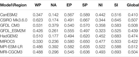
TABLE 1. Index of TC track density weighted by TC destructive potential for eight CMIP5 climate models in different areas and globe (WTD).

The distributions of TC-weighted track density simulated by individual models and their corresponding WTD scores indicate that the WTD score can effectively reflect the performance of these models in terms of TC track density and intensity. Results show that there exist large differences between different models for TC simulation in different areas. For example, the CSIRO Mk3.6.0 model can better simulate TCs in the WP, whereas it does the worst in the NA. It is worth noting that the algorithm for WTD calculation involves the identification of effective grid boxes, and the number of effective grids boxes are related to observations and simulations of the selected models in each area. Therefore, the scoring method in this study determines the performance of an individual model based on the WTD magnitude of its simulation relative to that of the other models in the same area. Thus, it makes no sense to compare absolute values of WTD between simulations in different areas. The proportions of PDI in individual regions to global total PDI (Figure 2) determined from observations are used as weighting factors of WTD scores in various areas to obtain the overall performance score for each model in each area (Table 1). In term of WTD scores, the MPI-ESM-LR demonstrates the best comprehensive performance (0.512), followed by the GFDL CM3, CSIRO Mk3.6.0, and MRI-CGCM3 (0.508, 0.507, 0.504). The CanESM2 performs the worst (0.410).

FIGURE 2

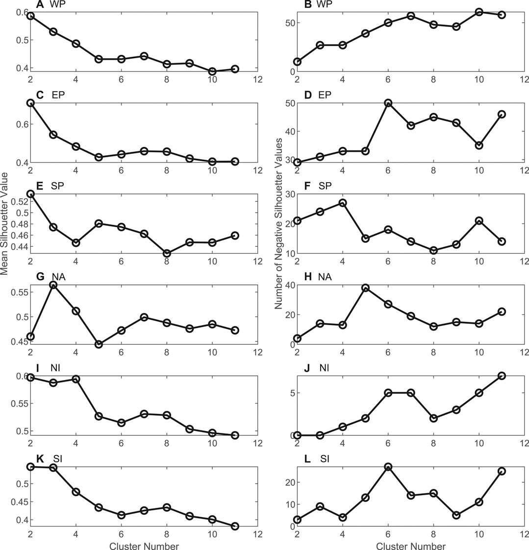
FIGURE 2. Changes in mean silhouette values for observed TCs in different areas (A,C,E,G,I, and K), and the number of negative silhouette values (B,D,F,H, and J) with the cluster number of TC track.

Simulation on Geographical Properties of TC Track

The average silhouette coefficients of characteristic TC track vectors in each area under different cluster numbers and the curves of the number of samples with silhouette coefficient less than 0 can be calculated using Eq. 3. Results are shown in Figure 2. According to the principle that the optimal cluster number corresponds to large average silhouette coefficient and to the smallest number of samples with silhouette coefficient less than 0, the optimal classification numbers of TC tracks in each area are obtained, which are 2 in the WP, EP, SP, SI, and NI, and 3 in the NA. Consistent with the setting in Shen et al. (2018), the weights of the three elements associated with the variance in different directions (i.e., zonal, meridional, and diagonal directions) and the other two elements associated with the centroid (i.e., latitude and longitude of the TC centroid) are set to 1/9 and 1/3 to weaken the effects of TC track pattern, length, and direction represented by the variances. Based on the number of clusters determined above, the k-means clustering method is applied to classify the observed TCs, and the initial center point of k-means cluster is randomly selected. The TC track classification in each area is obtained after repeated clustering. According to the latitude and longitude of multiple TC tracks of different track clusters, the average tracks for different classes of TC tracks in each area are obtained and displayed in Figure 3.

FIGURE 3

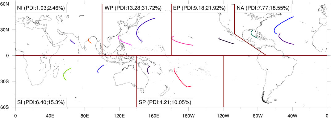
FIGURE 3. Distributions of mean tracks for various TC track clusters in different regions based on IBTrACS best-track data. The deep red line indicates the divisions of individual areas, and the color curves indicate the average tracks of TCs of different track clusters. The number in brackets indicates the PDI value in a specific area (units: 1013 m³ s⁻²) and its ratio to global total PDI.

The divisions of regions according to the IBTrACS standard are marked by lines in deep red color (Figure 3). Different color curves represent the average TC tracks of different clusters. In using the k-means clustering method, classification is based on internal similarity of the samples. Figure 3 shows that in each area, the observed TC track clusters obtained based on TC genesis position and track characteristics (e.g., length, pattern, and direction) demonstrate obvious differences. In the evaluation of model performance on the simulation of TC track classification, we compare the proportions of various TC track clusters simulated by the model with that of observations. According to the cluster centers of various TC track classes in different areas obtained from the observations, we calculate the Euclidean distances between multiple TC track vectors simulated by the eight models and individual cluster centers. The TC tracks are classified according to the shortest distance principle. Based on the classification results of TC tracks simulated by each model in different areas, the proportion of the number of TCs of various classes in an area simulated by the models to the total number of TCs in the area can be obtained. Using Eq. 2 in Shen et al. (2018), the GPT scores of each model in different areas and over the globe are calculated (Table 2). The closer the GPT value is to one, the closer the classification ratio of each track class simulated by this model is to the observations. In addition, the score has nothing to do with the number of simulated TCs, since it is solely determined by the TC track classification ratio.

TABLE 2

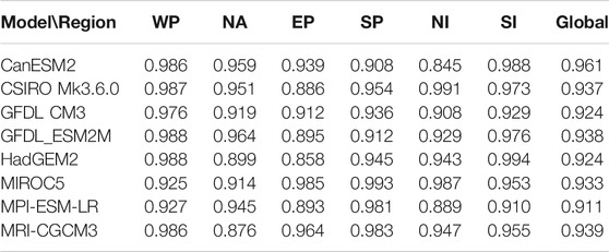
TABLE 2. Index of geographical properties of TC track for eight CMIP5 models in different areas and globe (GPT).

Table 2 shows clearly that in the WP, except for the MIROC5 and MPI-ESM-LR that have obvious lower scores for TC track classification, the scores of all the other models are very close. In other words, for the two clusters of TC tracks in the WP, although the numbers of TCs simulated by these models are significantly lower than the observation, most models can simulate the observed TC track classification ratio. In the EP, the GPT score of the MIROC5 model is the highest of 0.985, followed by the MRI-CGCM3 of 0.964. In the NA, the best model for the simulation of TC track classes is the GFDL_ESM2M (GPT of 0.964). Although the CanESM2 and CSIRO Mk3.6.0 models only simulate very few numbers of TCs in the NA, their performances are better than the MRI-CGCM3, which is the worst (GPT of 0.876). In the SP, the MIROC5 model is the best (GPT of 0.993), followed by the MPI-ESM-LR and MRI_CGCM43 models. In the SI, the HadGEM2 model yields the best simulation (0.994), followed by the CanESM2 model (0.988). In the NI, the CSIRO Mk3.6.0 model has the highest score of 0.991, followed by the MIROC5 model (0.987), and the CanESM2 model performs the worst (0.845). The GPT scores weighted by PDI in individual areas show that for the eight climate models, the CanESM2 model gives the best overall simulation of the TC track classification around the globe (0.961), and the MPI-ESM-LR model is the worst (0.911; Table 2).

Monthly Variation in the Proportion of TC Frequency

Figure 4 displays monthly variation of the ratio of TC frequency in each month to annual-mean TC frequency averaged over 1980–2005 for both observations and model simulations. The black curve in each panel represents observation, and color curves are model simulation results. Generally, these models have simulated the basic trend of monthly variation in TC frequency proportion in the six ocean areas. For example, in the Northern Hemisphere, TCs occur more frequently around August, except for the NI, where the two TC frequency peaks occur in May and October, respectively. In the Southern Hemisphere, TCs occur more frequently around January. Nevertheless, there are still differences between model simulations and observations. Compared with the other areas, the simulations in the WP, SP, and SI are better. All the models fail to simulate the peak values in July and August in the EP; and the simulated peaks occur in September and October instead. The differences between simulations and observations are more significant in the NA and NI than in the other areas.

FIGURE 4

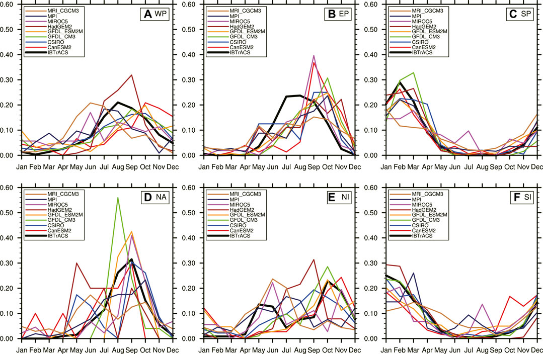
FIGURE 4. Variation in the proportion of monthly mean TC frequency to annual-mean TC frequency averaged over the period 1980–2015 in the six areas from observations and model simulations. The abscissa is month, and the ordinate is TC frequency proportion. The black curve represents observations, and the other curves represent the results of the eight CMIP5 models.

To quantitatively compare the model performance on simulating monthly variation of TC frequency proportion, we calculate the score for TC monthly frequency proportion. Table 3 shows that the scores in the WP, SP, and SI overall are higher than those in the other areas. This result is consistent with that shown in Figure 4. In the WP, the MVF is the highest for the CSIRO Mk3.6.0 model (0.971), and the second highest is the GFDL CM3 (0.963). In the EP, MVF values are similar for the MRI-CGCM3, MPI-ESM-LR, MIROC5, and GFDL_ESM2M, all showing relatively good simulations. In the SP, the CanESM2 has the highest MVF (0.979). In the NA, the MPI-ESM-LR (0.944) and GFDL_ESM2M (0.941) have relatively high values. In the NI, the CSIRO Mk3.6.0 model (0.944) and GFDL CM3 (0.943) have the highest MVF. In the SI, the GFDL CM3 has the highest MVF (0.988). Comparison of individual models shows that the CanESM2 performs the best in the SP and the second best in the NI. The CSIRO Mk3.6.0 model and GFDL CM3 both perform well in the SI and WP, while the GFDL_ESM2M and HadGEM2 perform well in the SP and SI. The MPI-ESM-LR performs the best in the SP, and the second best in the WP. The MRI-CGCM3 performs well in the SI. In summary, from the perspective of simulating monthly variation of TC frequency proportion, these models perform better in the SP and SI than in the other areas in the Southern Hemisphere; in the Northern Hemisphere, the simulations are the best in the WP. Considering the comprehensive results over all regions across the globe, the overall score is the best (0.932) for the CSIRO Mk3.6.0, followed by the GFDL CM3, GFDL_ESM2M, and MPI-ESM-LR, whose MVF scores are all of 0.930. The overall performance of the HadGEM2 (0.917) and MRI-CGCM3 (0.914) are relatively poor. Overall, there is no large difference in MVF among the various models.

TABLE 3

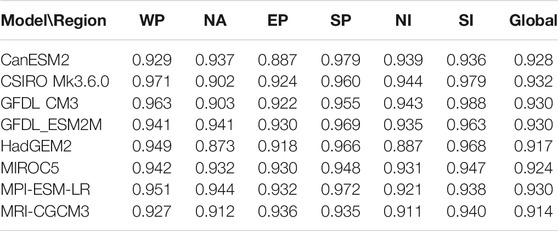
TABLE 3. Index of monthly variation of TC frequency proportion for eight CMIP5 models in different areas and globe (MVF).

Comprehensive Index

Values of the CEI obtained using Eq. 4 are listed in Table 4. Comprehensively considering the simulation of each model in terms of TC-weighted track density, TC track classification, and monthly variation in TC frequency proportion, it can be seen that in the WP the CSIRO Mk3.6.0 simulation is the best (0.597), the GFDL CM3 and HadGEM2 perform the second best (0.499 and 0.478, respectively), and the MIROC5 is the worst (0.287). In the NA, the simulations of the MPI-ESM-LR and GFDL CM3 are relatively good with the values of 0.349 and 0.315, respectively, and the other models are not ideal (all lower than 0.240). In the EP, the MIROC5 performs the best (0.532), followed by the MPI-ESM-LR and MRI-CGCM3 (0.484 and 0.492, respectively), which have similar scores. The HadGEM2 simulation is poor (0.389). In the SP, the CSIRO Mk3.6.0 and MIROC5 models demonstrate almost the same capability in terms of comprehensive simulation of TC-weighted track density, TC track classification, and monthly frequency proportion (both 0.611). Following the CSIRO Mk3.6.0 and MIROC5 models, the MPI-ESM-LR also shows relatively good capability (0.605). In the NI, the MIROC5 performs relatively well (0.438), followed by the MPI-ESM-LR and MRI-CGCM3 (0.427 and 0.425, respectively). In the SI, the HadGEM2 shows the best capability (0.658), while the MRI-CGCM3 and CSIRO Mk3.6.0 models are the second best (0.622 and 0.615, respectively). The global CEI score of each model is obtained using the PDI-weighted average of CEI scores in each area. As shown in Table 4, there are relatively small differences in global CEI scores (<0.1) despite the relatively large CEI differences in some areas (e.g., >0.3 in the WP) among the eight models. The four models with top CEI scores are the CSIRO Mk3.6.0 model, GFDL CM3, MPI-ESM-LR, and MRI-CGCM3 (0.443, 0.437, 0.434, and 0.433, respectively). The performances of the MIROC5 and CanESM2 are relatively poor (0.363 and 0.365, respectively).

TABLE 4

TABLE 4. Comprehensive evaluation index (CEI) for the eight CMIP5 models in different areas and globe.

Many previous studies have found that the model spatial resolution contributes significantly to model performance in simulating TC (e.g., Zhao et al., 2009; Murakami et al., 2015; Roberts et al., 2020; Tory et al., 2020). The above results also show that the models with relatively high horizontal resolution have relatively high scores. However, based on the model selected here, the correlation coefficient between the global CEI scores and the model resolution is not significant at the 90% confidence level. Moreover, the model with the highest resolution (i.e., MRI-CGCM3) does not have the highest score in simulating TCs. This maybe the fact that these CMIP5 climate models are all with spatial resolution of 1.1–2.5°, which are still too coarse to properly identify TC, so an increase in model resolution does not yield to a significant improvement in the performance of these models. In addition, dynamic cores of climate models and physical parameterization scheme will also affect the final simulation effect of TC (Zhang et al., 2021).

Conclusion

Different from the recent quantitative method to evaluate the capability of climate models in terms of TC simulation (Shen et al., 2018), the new method proposed in this study not only considers the capability of climate models for simulating density and geographical properties of TC tracks but also accounts for TC intensity and monthly variation characteristics of TC frequency. Moreover, the new method is applicable to TCs in regional oceans and over the globe. Specifically, compared with the method proposed by Shen et al. (2018), the new method has been optimized from three aspects. First, the method of Shen et al. (2018) can only assess the capability of climate models in simulating limited features of TC track, while the new method considers the TC destructive potential (the cube of the wind speed) in the calculation of TC track density, which actually implicitly considers TC intensity. Second, in terms of TC frequency simulation, a new evaluation component is added to consider the simulation of monthly variation of TC frequency. Third, the evaluation method for the WNP TCs in the previous study (Shen et al., 2018) is expanded to the global scale. Moreover, in the evaluation of the model capability for simulating global TC track classes, an objective approach (i.e., silhouette coefficient) is implemented to obtain the classification number of TC tracks in each ocean area. This number is later used in the k-means clustering. Furthermore, in calculating the score of model capability in TC simulation in each area, we do not consider the importance of each area equally. Instead, the PDI over the individual area is used as weighting coefficient to obtain the score for global simulation. This is because the PDI can reflect the destructive potential of TC, and we pay more attention to the regions with stronger potential damage by the TC.

After the optimization of the evaluation method in the above three aspects, this method is applied to the IBTrACS best-track data and TC simulations of eight CMIP5 models. Results of model simulations and observations are compared to obtain the ranking of model capability in simulating TC track density weighted by destructive potential, TC track classification, and monthly variation of TC frequency proportion. Large differences are found among model simulations of the above 3 TC features. In addition, the capabilities of the eight models are different in different areas. In the WP, the CSIRO Mk3.6.0 model performs the best; in the NA, the MPI-ESM-LR performs the best; in the EP, the MIROC5 is the best; in the SP, the CSIRO Mk3.6.0 and MIROC5 demonstrate the same capability, yet the CSIRO Mk3.6.0 model performs better in the simulation of TC-weighted track density and monthly variation of TC frequency proportion, while the MIROC5 performs better in simulating TC track classes. In the SI, the HadGEM2 performs the best. For the simulation over multiple areas across the globe, the CSIRO Mk3.6.0 model performs better overall, followed by the GFDL CM3, MPI-ESM-LR, and MRI-CGCM3.

he purposes of the present study are to optimize and to expand the objective method proposed in Shen et al. (2018) and to make it more effectively reflect the capability of climate models in terms of simulating TCs. The model capability in simulating multiple characteristics of TCs is comprehensively considered. The new method is applied to obtain performance scores of the eight CMIP5 models in six study areas. Obviously, the performances of these models are different in different areas. Therefore, when selecting models for follow-up research, appropriate climate models with better simulation capability should be selected based on the region of concern. Once the CMIP6 model outputs have been released fully, especially those variables used to identify TC tracks, we will use the newly proposed method to evaluate the performances of CMIP6 models.

Data Availability Statement

The best-track data is from the International Best Track Archive for Climate Stewardship (IBTrACS) dataset (https://www.ncdc.noaa.gov/oa/ibtracs/). Further inquiries can be directed to the corresponding author.

Author Contributions

YiS calculated the experimental data and wrote the paper. YuS, ZZ, and TL revised and optimized this paper.

Funding

This work is sponsored by China NSF Grants 42075035, 42088101, and 41675077.

Conflict of Interest

The authors declare that the research was conducted in the absence of any commercial or financial relationships that could be construed as a potential conflict of interest.

Publisher’s Note

All claims expressed in this article are solely those of the authors and do not necessarily represent those of their affiliated organizations, or those of the publisher, the editors and the reviewers. Any product that may be evaluated in this article, or claim that may be made by its manufacturer, is not guaranteed or endorsed by the publisher.

Acknowledgments

The authors thank Suzana J. Camargo for providing tropical cyclone track data tracking from CMIP5 climate model dataset.

References

Camargo, S. J. (2013). Global and Regional Aspects of Tropical Cyclone Activity in the CMIP5 Models. J. Clim. 26, 9880–9902. doi:10.1175/jcli-d-12-00549.1

CrossRef Full Text | Google Scholar

Camargo, S. J., Robertson, A. W., Gaffney, S. J., Smyth, P., and Ghil, M. (2007). Cluster Analysis of Typhoon Tracks. Part I: General Properties. J. Climate 20, 3635–3653.

Camargo, S. J., and Zebiak, S. E. (2002). Improving the Detection and Tracking of Tropical Cyclones in Atmospheric General Circulation Models. Wea. Forecast. 17, 1152–1162. doi:10.1175/1520-0434(2002)017<1152:itdato>2.0.co;2

CrossRef Full Text | Google Scholar

Caron, L.-P., Jones, C. G., and Winger, K. (2010). Impact of Resolution and Downscaling Technique in Simulating Recent Atlantic Tropical Cylone Activity. Clim. Dyn. 37 (5), 869–892. doi:10.1007/s00382-010-0846-7

CrossRef Full Text | Google Scholar

Chen, X., Zhong, Z., Zhong, Z., Hu, Y., Zhong, S., Lu, W., et al. (2019). Role of Tropical Cyclones over the Western North Pacific in the East Asian Summer Monsoon System. Earth Planet. Phys. 3 (2), 147–156. doi:10.26464/epp2019018

CrossRef Full Text | Google Scholar

Emanuel, K. A. (2005). Increasing Destructiveness of Tropical Cyclones Over the Past 30 Years. Nature 436, 686

Emanuel, K., Sundararajan, R., and Williams, J. (2008). Hurricanes and Global Warming: Results from Downscaling IPCC AR4 Simulations. Bull. Amer. Meteorol. Soc. 89, 347–368. doi:10.1175/bams-89-3-347

CrossRef Full Text | Google Scholar

Henderson-Sellers, A., Zhang, H., Berz, G., Emanuel, K., Gray, W., Landsea, C., et al. (1998). Tropical Cyclones and Global Climate Change: A post-IPCC Assessment. Bull. Amer. Meteorol. Soc. 79, 19–38. doi:10.1175/1520-0477(1998)079<0019:tcagcc>2.0.co;2

CrossRef Full Text | Google Scholar

Knapp, K. R., Kruk, M. C., Levinson, D. H., Diamond, H. J., and Neumann, C. J. (2010). The International Best Track Archive for Climate Stewardship (IBTrACS). Bull. Amer. Meteorol. Soc. 91, 363–376. doi:10.1175/2009bams2755.1

CrossRef Full Text | Google Scholar

Kossin, J. P., Emanuel, K. A., and Camargo, S. J. (2016). Past and Projected Changes in Western North Pacific Tropical Cyclone Exposure. J. Clim. 29, 5725–5739. doi:10.1175/jcli-d-16-0076.1

CrossRef Full Text | Google Scholar

LaRow, T. E., Lim, Y.-K., Shin, D. W., Chassignet, E. P., and Cocke, S. (2008). Atlantic basin Seasonal hurricane Simulations. J. Clim. 21, 3191–3206. doi:10.1175/2007jcli2036.1

CrossRef Full Text | Google Scholar

Manganello, J. V., Hodges, K. I., Kinter, J. L., Cash, B. A., Marx, L., Jung, T., et al. (2012). Tropical Cyclone Climatology in a 10-km Global Atmospheric GCM: toward Weather-Resolving Climate Modeling. J. Clim. 25, 3867–3893. doi:10.1175/jcli-d-11-00346.1

CrossRef Full Text | Google Scholar

Murakami, H., Vecchi, G. A., Underwood, S., Delworth, T. L., Wittenberg, A. T., Anderson, W. G., et al. (2015). Simulation and Prediction of Category 4 and 5 Hurricanes in the High-Resolution GFDL HiFLOR Coupled Climate Model. J. Clim. 28, 9058–9079. doi:10.1175/jcli-d-15-0216.1

CrossRef Full Text | Google Scholar

Nakamura, J., Lall, U., Kushnir, Y., and Camargo, S. J. (2009). Classifying North Atlantic Tropical Cyclone Tracks By Mass Moments. J. Climate 22, 5481–5494.

Peduzzi, P., Chatenoux, B., Dao, H., De Bono, A., Herold, C., Kossin, J., et al. (2012). Global Trends in Tropical Cyclone Risk. Nat. Clim Change 2 (4), 289–294. doi:10.1038/nclimate1410

CrossRef Full Text | Google Scholar

Peter, R. J. (1987). Silhouettes: A Graphical Aid to the Interpretation and Validation of Cluster Analysis. J. Comput. Appl. Maths. 20, 53–65. doi:10.1016/0377-0427(87)90125-7

CrossRef Full Text | Google Scholar

Pielke, R. A., Gratz, J., Landsea, C. W., Collins, D., Saunders, M. A., and Musulin, R. (2008). Normalized Hurricane Damage in the United States: 1900-2005. Nat. Hazards Rev. 9 (1), 29–42. doi:10.1061/(asce)1527-6988(2008)9:1(29)

CrossRef Full Text | Google Scholar

Rappaport, E. N. (2014). Fatalities in the United States from Atlantic Tropical Cyclones: New Data and Interpretation. Bull. Am. Meteorol. Soc. 95 (3), 341–346. doi:10.1175/bams-d-12-00074.1

CrossRef Full Text | Google Scholar

Roberts, M. J., Camp, J., Seddon, J., Vidale, P. L., Hodges, K., Vanniere, B., et al. (2020). Impact of Model Resolution on Tropical Cyclone Simulation Using the HighResMIP-PRIMAVERA Multimodel Ensemble. J. Clim. 33, 2557–2583. doi:10.1175/jcli-d-19-0639.1

CrossRef Full Text | Google Scholar

Shaevitz, D. A., Camargo, S. J., Sobel, A. H., Jonas, J. A., Kim, D., Kumar, A., et al. (2014). Characteristics of Tropical Cyclones in High‐resolution Models in the Present Climate. J. Adv. Model. Earth Syst. 6, 1154–1172. doi:10.1002/2014ms000372

CrossRef Full Text | Google Scholar

Shen, Y., Sun, Y., Camargo, S. J., and Zhong, Z. (2018). A Quantitative Method to Evaluate Tropical Cyclone Tracks in Climate Models. J. Atmos. Oceanic Technol. 35 (9), 1807–1818. doi:10.1175/jtech-d-18-0056.1

CrossRef Full Text | Google Scholar

Song, Y., Wang, L., Lei, X., and Wang, X. (2015). Tropical Cyclone Genesis Potential index over the Western North Pacific Simulated by CMIP5 Models. Adv. Atmos. Sci. 32, 1539–1550. doi:10.1007/s00376-015-4162-3

CrossRef Full Text | Google Scholar

Strazzo, S., Elsner, J. B., Larow, T., Halperin, D. J., and Zhao, M. (2013). Observed versus GCM-Generated Local Tropical Cyclone Frequency: Comparisons Using a Spatial Lattice. J. Clim. 26 (21), 8257–8268. doi:10.1175/jcli-d-12-00808.1

CrossRef Full Text | Google Scholar

Taylor, K. E. (2001). Summarizing Multiple Aspects of Model Performance in a Single Diagram. J. Geophys. Res. 106 (D7), 7183–7192. doi:10.1029/2000jd900719

CrossRef Full Text | Google Scholar

Tonkin, H., Landsea, C., Holland, G. J., and Li, S. (1997). “Tropical Cyclones and Climate Change: A Preliminary Assessment,”. Assessing Climate Change: Results from the Model Evaluation Consortium for Climate Assessment. Editors W. Howe, and A. Henderson-Sellers (Sydney: Gordon & Breach), 327–360.

Google Scholar

Tory, K. J., Ye, H., and Brunet, G. (2020). Tropical Cyclone Formation Regions in CMIP5 Models: a Global Performance Assessment and Projected Changes. Clim. Dyn. 55, 3213–3237. doi:10.1007/s00382-020-05440-x

CrossRef Full Text | Google Scholar

Zhang, W., Villarini, G., Scoccimarro, E., Roberts, M., Vidale, P. L., Vanniere, B., et al. (2021). Tropical Cyclone Precipitation in the HighResMIP Atmosphere-Only Experiments of the PRIMAVERA Project. Clim. Dyn. 57, 253–273. doi:10.1007/s00382-021-05707-x

CrossRef Full Text | Google Scholar

Zhao, M., and Held, I. M. (2010). An Analysis of the Effect of Global Warming on the Intensity of Atlantic Hurricanes Using a GCM with Statistical Refinement. J. Clim. 23, 6382–6393. doi:10.1175/2010jcli3837.1

CrossRef Full Text | Google Scholar

Zhao, M., Held, I. M., Lin, S.-J., and Vecchi, G. A. (2009). Simulations of Global hurricane Climatology, Interannual Variability, and Response to Global Warming Using a 50-km Resolution GCM. J. Clim. 22, 6653–6678. doi:10.1175/2009jcli3049.1

CrossRef Full Text | Google Scholar

Zhou, B. T. (2012). Model Evaluation and Projection on the Linkage between Hadley Circulation and Atmospheric Background Related to the Tropical Cyclone Frequency over the Western North Pacific. Atmos. Oceanic Sci. Lett. 5, 473–477. doi:10.1080/16742834.2012.11447036

CrossRef Full Text | Google Scholar

Zhou, B., and Xu, Y. (2017). How the "best" CMIP5 Models Project Relations of Asian-Pacific Oscillation to Circulation Backgrounds Favorable for Tropical Cyclone Genesis over the Western North Pacific. J. Meteorol. Res. 31, 107–116. doi:10.1007/s13351-017-6088-4

CrossRef Full Text | Google Scholar