The Nonlinear Radiative Feedback Effects in the Arctic Warming

The analysis of radiative feedbacks requires the separation and quantification of the radiative contributions of different feedback variables, such as atmospheric temperature, water vapor, surface albedo, cloud, etc. It has been a challenge to include the nonlinear radiative effects of these variables in the feedback analysis. For instance, the kernel method that is widely used in the literature assumes linearity and completely neglects the nonlinear effects. Nonlinear effects may arise from the nonlinear dependency of radiation on each of the feedback variables, especially when the change in them is of large magnitude such as in the case of the Arctic climate change. Nonlinear effects may also arise from the coupling between different feedback variables, which often occurs as feedback variables including temperature, humidity and cloud tend to vary in a coherent manner. In this paper, we use brute-force radiation model calculations to quantify both univariate and multivariate nonlinear feedback effects and provide a qualitative explanation of their causes based on simple analytical models. We identify these prominent nonlinear effects in the CO₂-driven Arctic climate change: 1) the univariate nonlinear effect in the surface albedo feedback, which results from a nonlinear dependency of planetary albedo on the surface albedo, which causes the linear kernel method to overestimate the univariate surface albedo feedback; 2) the coupling effect between surface albedo and cloud, which offsets the univariate surface albedo feedback; 3) the coupling effect between atmospheric temperature and cloud, which offsets the very strong univariate temperature feedback. These results illustrate the hidden biases in the linear feedback analysis methods and highlight the need for nonlinear methods in feedback quantification.

Introduction

Radiative forcing and feedbacks strongly influence the Arctic climate. The warming in the Arctic has occurred in a faster pace than the global average, due to greenhouse gas forcing and amplifying feedbacks (Stocker et al., 2013). It requires accurate quantification of the radiative effects of associated feedback variables (surface albedo, atmospheric temperature, water vapor, cloud, etc.,) in order to ascertain their contributions to the climate change of interest. For instance, based on the energy budget balance with regard to the Top-of-Atmosphere (TOA), surface or atmospheric budget and assuming the warming induced thermal radiation (Planck effect) balances the radiation changes caused by feedbacks, one can infer how much global or regional warming, e.g., the Arctic warming amplification, can be attributed to individual feedbacks (Held and Soden 2000; Lu and Cai 2009; Pithan and Mauritsen 2014).

Often assumed in feedback analysis is linear additivity of the radiative effects of different feedback variables. For instance, the widely adopted kernel method (Soden and Held 2006) measures the radiation change caused by a feedback variable ($X$) by multiplying a pre-calculated radiative kernel ($\frac{\partial R}{\partial X}$) with the climate response ($dX$). Due to its simple concept and computational efficiency, a large number of studies have been conducted using this method (e.g., Soden and Held 2006; Zelinka et al., 2012; Vial et al., 2013; Zhang and Huang, 2014) and pre-computed kernels based on different atmospheric datasets, including climate models, reanalyses and satellite data (e.g., Soden et al., 2008; Yue et al., 2016; Huang et al., 2017).

The nonlinear effects, however, are often too large to ignore. When individual feedback terms are independently measured, such as the non-cloud feedbacks in the clear-sky case in the kernel method, the ignored nonlinear effects may lead to a non-closure of the radiation budget, i.e., the sum of the individual terms cannot reproduce the overall radiation change (e.g., Huang 2013; Vial et al., 2013). In the Arctic, where climate perturbations are of large magnitudes, e.g., in the case of sea ice melt, the non-closure issue is especially noticeable (e.g., Shell et al., 2008; Block and Mauritsen 2013; Zhu et al., 2019). Besides the large perturbations in surface albedo, the Arctic is also noted for its strong and unique lapse rate (e.g., Pithan and Mauritsen 2014) and cloud (e.g., Kato et al., 2006) feedbacks. It should be noted that although some methods exhibit a seemingly good radiation closure, the nonlinear effects are not treated but hidden in the feedback term(s) measured as a residual, e.g., the cloud feedback term in the typical kernel method, including the adjusted cloud radiative forcing (aCRF) technique (Shell et al., 2008; Soden et al., 2008).

Although the existence of the nonlinear effects has been recognized (e.g., Zhang et al., 1994; Colman et al., 1997), their impacts were seldom isolated and quantified. Some recent works have specifically addressed the nonlinearity issue in the radiative feedback analysis. Zhu et al. (2019) for the first time used a neural network model (a nonlinear diagnostic method without linearity assumption) to assess the radiative feedbacks and identified a few strong nonlinear effects, including a strong cloud-water vapor coupling effect in the tropical climate variations and a strong nonlinear dependence of radiation flux on the surface albedo. Using Partial-Radiative-Perturbation (PRP) experiments and brute-force radiation model-based computations, Huang and Huang (2021) verified the cloud-water vapor coupling effect and offered an analytic estimation of this effect on the longwave radiation. Shakirova and Huang (2021) advanced the neural network model of Zhu et al. and demonstrated its advantages particularly for quantifying the albedo feedback.

In this paper, we aim to give an overview of the nonlinear radiative feedback effects in Arctic climate change. Based on a heuristic climate change scenario of broad interest: the abrupt quadrupling of atmospheric CO₂ (4xCO₂), we investigate how the nonlinear radiative effects arise from the univariate and multivariate variations of the feedback variables, such as atmospheric and surface temperature (t), water vapor (q), surface albedo (a) and cloud (c), and measure how the nonlinear effects compare to the linear effects in terms of magnitude and pattern. We note that in this paper we are not concerned with how the changes in these variables are resulted, which if nonlinearly related to the surface warming may also cause nonlinearity in climate feedbacks, but focus on how their changes, as projected by the GCM, lead to nonlinear changes in the TOA longwave (LW) and shortwave (SW) radiation energy fluxes. In the following sections, we will define, demonstrate and discuss the various feedback effects of interest in order.

Method: Feedback Definitions

Here, we define a radiative feedback as the (partial) radiation change, in the units of W m⁻², due to one or multiple feedback variables. This should be distinguished from a feedback parameter, which is normalized by surface temperature change and is in the units of W m⁻² K⁻¹.

Consider the radiation field of interest, e.g., the TOA or surface radiation flux, as a function of the feedback variables: $R=R\left(x, y, z\right)$, where the letters ($x, y, z$) are generic notations of the feedback variables. The total radiation change in a given climate change scenario can thus be expressed by a Taylor series as

$\begin{array}{c}\Delta R_{(x,y,z)}=R\left(x_2, y_2, z_2\right)-R\left(x_1, y_1, z_1\right)\\ =\frac{\partial R}{\partial x}\Delta x+\frac{\partial R}{\partial y}\Delta y+\frac{\partial R}{\partial z}\Delta z\hspace{1em}\hspace{1em}\hspace{1em}\left(\mathrm{univariate linear effects}\right)\\ +\frac{1}{2}[\frac{{\partial }^{2}R}{\partial x^2}{\left(\Delta x\right)}^2+\frac{{\partial }^{2}R}{\partial y^2}{\left(\Delta y\right)}^2+\frac{{\partial }^{2}R}{\partial z^2}{\left(\Delta z\right)}^2\hspace{1em}\left(\mathrm{univariate nonlinear effects}\right)\\ +2\frac{{\partial }^{2}R}{\partial x\partial y}\Delta x\Delta y+2\frac{{\partial }^{2}R}{\partial y\partial z}\Delta y\Delta z+2\frac{{\partial }^{2}R}{\partial x\partial z}\Delta x\Delta z]\hspace{0.17em}\hspace{0.17em}\hspace{0.17em}\hspace{0.17em}\hspace{0.17em}\left(\mathrm{multivariate nonlinear effects}\right)\\ + O\left({\Delta }^3 \right)\end{array}(1)$

where the subscripts 1 and 2 denote two different climate states, e.g., those before and after quadrupling CO₂ (noted as 1xCO₂ and 4xCO₂, respectively from now on); such terms as $\Delta x=x_2-x_1$ denote the climate responses. The terms on the righthand side of Eq. (1) illustrate three types of radiative effects that we aim to elucidate here:

1) The univariate linear effects, such as $\frac{\partial R}{\partial x}\Delta x$, which we denote as $\Delta R_x$;

2) The univariate nonlinear effects, such as $\frac{1}{2}\frac{{\partial }^{2}R}{\partial x^2}{\left(\Delta x\right)}^2$, which we denote as $\Delta R_{xx}$;

3) The multivariate nonlinear effects, such as $\frac{{\partial }^{2}R}{\partial x\partial y}\Delta x\Delta y$, which we denote as $\Delta R_{xy}$.

To avoid confusion, we denote a univariate feedback, i.e., the overall radiation change due to a single variable, as $\Delta R_{\left(x\right)}$, which consists of both univariate linear ($\Delta R_x$) and univariate nonlinear ($\Delta R_{xx}$) effects:

$\begin{array}{c}\Delta R_{\left(x\right)}=R\left(x_2, y_1,\mathrm{...}\right)-R\left(x_1, y_1,\mathrm{...}\right)\\ =\frac{\partial R}{\partial x}\Delta x+\frac{1}{2}\frac{{\partial }^{2}R}{\partial x^2}{\left(\Delta x\right)}^2+O\left({\Delta }^3\right)\\ =\Delta R_x+\Delta R_{xx}\end{array}(2)$

Equation (2) is written following the PRP concept (Wetherald and Manabe 1988) and measures the univariate feedbacks by simply evaluating the radiation flux twice: first with an unperturbed profile, $R\left(x_1, y_1,\mathrm{...}\right)$, and then perturbing x only, $R\left(x_2, y_1,\mathrm{...}\right)$. Note that other unperturbed independent variables than y are omitted in these expressions. If not otherwise stated, unspecified independent variables all take the unperturbed values when the radiation fluxes are evaluated in the following. The evaluation of the radiation fluxes can be done using a physical model, i.e., a radiative transfer model (RTM) (Huang and Huang 2021), or a statistical model, e.g., a neural network model that emulate the radiation fluxes (Zhu et al., 2019).

Similarly, a bivariate feedback can be expressed as:

$\begin{array}{c}\Delta R_{\left(x,y\right)}=R\left(x_2, y_2\right)-R\left(x_1, y_1\right)\\ =\frac{\partial R}{\partial x}\Delta x+\frac{\partial R}{\partial y}\Delta y+\frac{1}{2}\frac{{\partial }^{2}R}{\partial x^2}{\left(\Delta x\right)}^2+\frac{1}{2}\frac{{\partial }^{2}R}{\partial y^2}{\left(\Delta y\right)}^2+\frac{{\partial }^{2}R}{\partial x\partial y}\Delta x\Delta y+O\left({\Delta }^3\right)\\ =\Delta R_x+\Delta R_y+\Delta R_{xx}+\Delta R_{yy}+\Delta R_{xy}\end{array}(3)$

From Eq. 2 and Eq. 3, the bivariate coupling effect $\Delta R_{xy}$ can be obtained as

$\begin{array}{c}\Delta R_{xy}=\Delta R_{\left(x,y\right)}-\Delta R_{\left(x\right)}-\Delta R_{\left(y\right)}\\ =R\left(x_2, y_2\right)-R\left(x_2, y_1\right)-R\left(x_1, y_2\right)+R\left(x_1, y_1\right)\end{array}(4)$

Based on the above equations and following Huang and Huang (2021), we evaluate the radiation fluxes and isolate the respective feedback effects $\left(\Delta R_x, \Delta R_{xx}, \Delta R_{xy}, etc.\right)$, using the Rapid Radiative Transfer Model (RRTM, Mlawer et al., 1997). Using this RTM, the TOA and surface radiation fluxes are computed offline from instantaneous atmospheric profiles generated by the Community Earth System Model, CESM1.2, in a quadrupling CO₂ experiment (Wang and Huang, 2020). More details of the flux computation can be found in Huang and Huang (2021); we note that the radiative transfer computations, including the PRP computations, are based on instantaneous (3-hourly, as opposed to monthly mean) profiles at the original horizontal resolutions (1.9 ° × 2.5 °) of the CESM and then averaged monthly or annually in all the results presented in the following section.

Note that we use a one-sided PRP, starting with the unperturbed climate and then prescribing the change(s) in the variables of interest, to define feedbacks, i.e., how much radiation change is caused by the change of the feedback variable(s) of concern. Some studies opt to use two-sided perturbations (e.g., Colman and McAvaney 1997). In contrast to Eq. (2), one may evaluate the feedback of x as

$\begin{array}{c}\delta R_{\left(x\right)}=\frac{1}{2}R\left[\left(x_2, y_1\right)-R\left(x_1, y_1\right)+R\left(x_2, y_2\right)-R\left(x_1, y_2\right)\right]\\ \approx \frac{1}{2}[{\frac{\partial R}{\partial x}|}_{y1}\Delta x+{\frac{\partial R}{\partial x}|}_{y2}\Delta x]\approx \frac{1}{2}[{\frac{\partial R}{\partial x}|}_{y1}\Delta x+\left({\frac{\partial R}{\partial x}|}_{y1}+{\frac{\partial }{\partial y}\left(\frac{\partial R}{\partial x}\right)|}_{y1}\Delta y\right)\Delta x\\ =\frac{\partial R}{\partial x}+\frac{1}{2}\frac{{\partial }^{2}R}{\partial x\partial y}\Delta x\Delta y\end{array}(5)$

which, as shown in the above expansion, effectively includes nonlinear coupling effects such as $\frac{1}{2}\frac{{\partial }^{2}R}{\partial x\partial y}\Delta x\Delta y$ in $\delta R_{\left(x\right)}$. When individual feedbacks are evaluated this way, their sum can better reproduce the overall radiation change, i.e., achieving a better radiation closure. However, it should be noted these "individual" feedbacks $\delta R_{\left(x\right)}$ differ from the univariate feedbacks $\Delta R_{\left(x\right)}$ as $\delta R_{\left(x\right)}$ contains coupling effects. To disclose these coupling effects, we adopt the one-sided formulations as exemplified by Eq. 2, Eq. 3, and Eq. 4

Results

In this paper, we use the climate change in an abrupt 4xCO₂ experiment of CESM (Wang and Huang, 2020) to provide a context for examining the linear and nonlinear radiative feedbacks. As illustrated in Figure 1 for a few selected variables, this scenario represents strong perturbations in the Arctic climate, including reduction in surface albedo due to sea ice melt, surface warming and atmospheric moistening. The feedback quantifications presented in the following are based on the two months exemplified in Figure 1 if not otherwise noted.

FIGURE 1

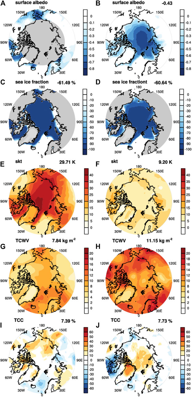
FIGURE 1. Changes in climate variables in the 4xCO₂ experiment, exemplified by two months a January (left column) and a June (right column). (A,B) Suface albedo; (C,D) sea ice fraction; (E,F) surface skin temperature; (G,H) column-integrated water vapor; (I,J) total cloud fraction. The numbers on the upper right corner of each panel are the Arctic mean values, averaged over the latitude range of 70–90°N. Shaded in grey are regions with no data, for instance, due to no solar insolation to infer surface albedo in (A).

Univariate Linear Effects

The univariate linear effect $\Delta R_x$ can be measured, following its definition, by multiplying the radiative linear sensitivity kernel $K_x=\frac{\partial R}{\partial x}$ with the climate response $\Delta x\mathrm{:}{R}_x=K_x\Delta x$. This is the core idea of the kernel method (Soden et al., 2008). The kernels are usually pre-computed, again, following the PRP idea, by prescribing small perturbations to the individual variables, e.g., 1-K in atmospheric and surface temperatures, several percent change in water vapor concentration, or 0.01 increment of surface albedo (e.g., Shell et al., 2008):

$K_x=\frac{\Delta R_0}{\Delta x_0}=\frac{R\left(x_1+\Delta x_0, y_1\right)-R\left(x_1, y_1\right)}{\Delta x_0}(6)$

so that the kernel method is in essence to scale up the radiation change due to an infinitesimal (small) perturbation, $R_0$, to estimate the radiation change due to a finite (large) perturbation:

$\Delta R_x=K_x\Delta x=\Delta R_0\frac{\Delta x}{\Delta x_0}(7)$

It is worth noting that when defining and applying the kernels, it is advisable to choose a scaling scheme appropriate to the radiation dependency on the feedback variable. For instance, in the case of such greenhouse gases as carbon dioxide and water vapor, their radiative effects are logarithmically dependent on their concentrations (e.g., Bani Shahabadi and Huang., 2014), so that it is common to define the water vapor kernel with respect to the change in the logarithm of the specific humidity, i.e., $K_q=\frac{\Delta R_0}{\Delta {\left(ln\left(q\right)\right)}_0}$, or, in an approximate form, using the fractional change in q in the denominator, i.e., $K_q=\frac{\Delta R_0}{{\left(\Delta q/q\right)}_0}$. As shown by Figure 2, using the logarithmic scaling scheme, the radiation change caused by water vapor perturbations, even when the perturbations are of large magnitudes (about 200% increase of TCWV), can be well approximated according to Eq. (7).

FIGURE 2

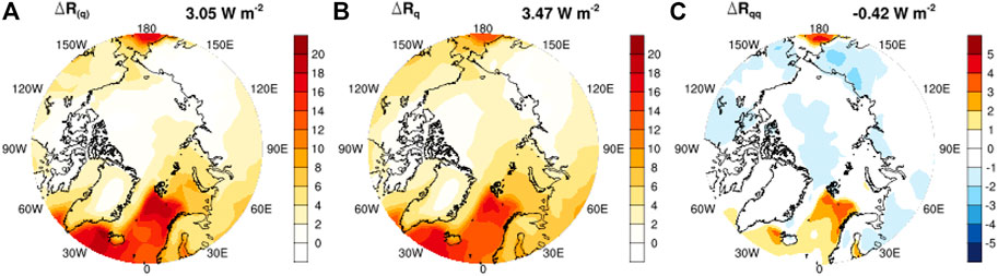
FIGURE 2. Clear-sky univariate water vapor LW feedback. (A) RTM-computed (truth) overall univariate feedback, $\Delta R_{\left(q\right)}$; (B) kernel-estimated univriate linear feedback, $\Delta R_q$, based on logarithmic scaling; (C) the residual (A–B), i.e., the univariate nonlinear feedback, $\Delta R_{qq}$. Shown here is the clear-sky TOA LW radiation flux change due to the water vapor change in January in the 4xCO₂ experiment (as illustrated in Figure 1E). The kernel used in (B) is computed from the GCM instantaneous atmospheric profiles of the same month and is not subject to the bias discussed in Eq. 8.

The validations against RTM-computed truth in Figures 2, 3 show that the non-cloud univariate radiative feedbacks $\Delta R_{\left(x\right)}$, even in the case of large climate perturbations, can be reasonably approximated by the linear term $\Delta R_x$. This is the basis of the kernel method (Soden et al., 2008). Nevertheless, the biases, i.e., the univariate nonlinear effects $\Delta R_{xx}$ may amount to non-negligible extent: in the case of the univariate water vapor feedback and the surface albedo feedback, the biases can amount to more than 10% in terms of Arctic mean (averaged over 70–90°N).

FIGURE 3

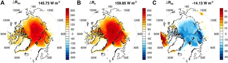
FIGURE 3. All-sky univariate surface albedo SW feedback. (A) RTM-computed (truth), $\Delta q{R}_{\left(a\right)}$; (B) kernel-estimated univariate linear feedback,$\Delta R_a$; and (C) the residual (A–B), i.e., the univariate nonlinear term $\Delta R_{aa}$. Shown here is the all-sky TOA SW radiation flux change due to the surface albedo change in June in the 4xCO₂ experiment (as illustrated in Figure 1B).

It should be cautioned that the kernel itself has a dependency on the atmospheric conditions (x, y, z, … ) and such dependency should be recognized when interpreting the kernel-diagnosed feedbacks. The kernels appropriate to evaluating the linear feedbacks in Eq. 1, Eq. 2, and Eq. 3, and used to compute $\Delta R_q$ in Figure 2 and $\Delta R_a$ in Figure 3, are computed from the GCM atmopsheric profiles in the unperturbed (1xCO2) climate, i.e., $K_x={\frac{\partial R}{\partial x}|}_{x_1,y_1,z_1}$, where ($x_1,y_1,z_1$) denotes the 1xCO₂ climate. If computed from different atmospheric states, the kernel values may quantitatively differ (e.g., see the kernel comparisons in Huang et al., 2017; Smith et al., 2020 and others). If a kernel computed from a different atmospheric state $(x_1^{\prime },y_1^{\prime },z_1^{\prime })$ is used to measure the linear feedback, a bias is resulted:

$\begin{array}{c}\Delta R_x^{\prime }={\frac{\partial R}{\partial x}|}_{x_1^{\prime },y_1^{\prime },z_1^{\prime }}\Delta x\\ \approx \left({\frac{\partial R}{\partial x}|}_{x_1,y_1,z_1}+{\frac{{\partial }^{2}R}{\partial x^2}|}_{x_1,y_1,z_1}d{x}^{\prime }+{\frac{{\partial }^{2}R}{\partial x\partial y}|}_{x_1,y_1,z_1}d{y}^{\prime }+{\frac{{\partial }^{2}R}{\partial x\partial z}|}_{x_1,y_1,z_1}d{z}^{\prime }\right)\Delta x\\ =\Delta R_x+bias\end{array}(8)$

Equation (8) shows that the bias can be considered one type of nonlinear effect in that it, like the nonlinear effects analyzed below, results from the nonlinear dependency of the radiation on the feedback variables (e.g., $\frac{{\partial }^{2}R}{\partial x\partial y}$). For the simplicity of the expressions, we omit the notation ${\left(\mathrm{...}\right)|}_{x_1,y_1,z_1}$ in the following, where the conditioned states can be inferred from the context.

The magnitude of the feedback bias caused by kernel bias is proportional to the discrepancies in the atmospheric states ($d{x}^{\prime }$, $d{y}^{\prime }$, and $d{z}^{\prime }$ in Eq. (8)), which may introduce noticeable quantitative differences in the kernels. For example, one may see from Fig. S3 of Huang et al. (2017), as well as the discussions of Sanderson and Shell (2012), the temperature kernel discrepancies due to the ubiquitous discrepancies in the cloud distribution in different atmospheric datasets used for kernel computation. Here, as a sanity check, we recalculate the Arctic mean clear-sky water vapor feedback shown in Figure 2 using the clear-sky kernels of Huang et al. (2017) and obtain an Arctic mean $\Delta R_q$ of 5.79 W m⁻² (Figure 4). This, compared to the RTM-computed truth value of 3.05 W m⁻², representes a 90% bias and is much larger than the bias when the correct (GCM 1xCO₂ climate based) kernels are used (3.47 W m⁻², as shown by Figure 2B). The results indicates that, contradictory to common belief, there may be large biases, especially in regional (e.g., Arctic) feedbacks, resulting from kernel biases.

FIGURE 4

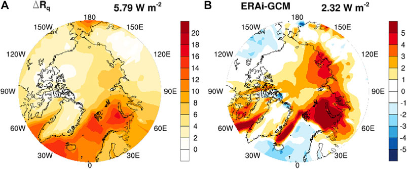
FIGURE 4. Clear-sky water vapor feedback bias due to kernel bias. (A) Like Figure 2B, but using the kernels computed from different atmospheric profiles (Huang et al., 2017); (B) Bias compared to Figure 2B.

Lastly, we note that cloud feedback is difficult, if not impossible, to be approximated by linear kernels. This is because cloud variations involve multiple radiative properties, including cloud fraction, droplet concentration and size distribution, etc., each of which may experience large, discrete perturbations and strongly affect the radiative sensitivity to each other. The cloud radiative effects measured in the cloud property histogram method (Zelinka et al., 2012) illustrate how the radiative sensitivity to cloud varies strongly with the cloud properties. Among other issues, a notable challenge is the vertical masking effect: for instance, the increase of upper-level clouds greatly reduces the sensitivity of the TOA fluxes to the lower-level clouds.

In summary, the non-cloud univariate feedbacks in general can be approximated well by the kernel method, although one should be mindful about the biases introduced by kernel discrepancies. One most noticeable univariate nonlinear effect in the Arctic is the surface albedo feedback. We further analyze this and other nonlinear effects in the following subsections.

Univariate Nonlinear Effects

Because radiative transfer is a complex nonlinear process (e.g., see Goody and Yung 1989), atmospheric radiation fluxes generally have a nonlinear dependency on the feedback variables and thus the univariate nonlinear effects generally exist.

Temperature

With regard to the univariate temperature feedback, a well-recognized cause of the nonlinearity is the Planck function, although this nonlinearity is weak at the terrestrial temperatures. Based on the Stefan-Boltzmann Law,

$R=\sigma t^4(9)$

Given the constant $\sigma$ = 5.67 × 10⁻⁸ W m⁻² K⁻⁴, one may find that the nonlinear effect $\frac{{\partial }^{2}R}{\partial t^2}$ is only about 1% of the linear effect $\frac{\partial R}{\partial t}$, for a 1-K perturbation around the equivalent blackbody temperature of Earth (t = 255K). Another cause of the nonlinearity is the dependence of the gas absorptivity on the temperature, which also has a minor impact (Huang et al., 2007). This explains why the temperature feedback in the case of large perturbations can still be very well approximated by the linear kernels (not shown).

Water Vapor

The univariate water vapor feedback is generally well estimated when the logarithmic scaling scheme is used, although Figure 2C shows that the bias (i.e., the univariate nonlinear effect, $\Delta R_{qq}$) can be non-negligible. A notable reason that causes the feedback to deviate from the logarithmic behavior is the unsaturated atmospheric absorption in the mid-infrared window around 10 μm wavelength. Here, the surface emission strongly contributes to the OLR and thus the water vapor feedback cannot be interpreted simply as the elevation of the atmospheric emission level, which gives rise to the logarithmic dependence (Bani Shahabadi and Huang., 2014). Figure 5 suggests that the water vapor feedback estimation may be improved if different scaling schemes are used for different spectral bands: logarithmic in the absorption bands (where atmospheric optical depth is large) and linear in the window bands (where optical depth is small):

$\Delta R_{\left(q\right)}=K_q^{log}\Delta \left(ln\left(q\right)\right)+K_q^{lin}\Delta q(10)$

where the logarithmic kernel $K_q^{log}$ accounts for the logarithmic response of the radiation flux in the absorption bands to water vapor perturbation and the linear kernel $K_q^{lin}$ accounts for the linear response in the window band. Further research is required to develop and validate a global hybrid kernel set.

FIGURE 5

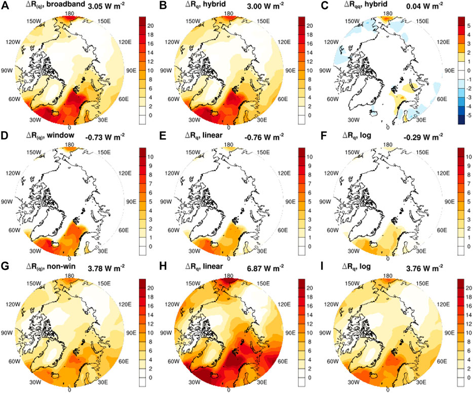
FIGURE 5. Spectral breakdown of the clear-sky univariate water vapor feedback. (A) RTM-computed (truth) broadband univariate feedback, $\Delta R_{\left(q\right)}$; (B) kernel-diagnosed broadband feedback, $\Delta R_q$, using the hybrid scaling (Eq. 10); (C) residual, $\Delta R_{qq}$. (D–F) Window band (700–1,180 cm⁻¹) feedback, computed by RTM and estimated by linear and logarithmic scaling. (G–I) Like (D–F), but for the non-window (absorption) bands.

Surface Albedo

The univariate surface albedo feedback shows especially strong nonlinear dependence on the surface albedo a (Figure 6). This is because the multiple scattering of radiation between the surface and atmosphere renders a nonlinear dependency of planetary albedo on surface albedo. Following Stephens et al. (2015), the planetary albedo $a_p$ can be expressed as

$a_p=r+\frac{a{\tau }^2}{1-ra}(11)$

FIGURE 6

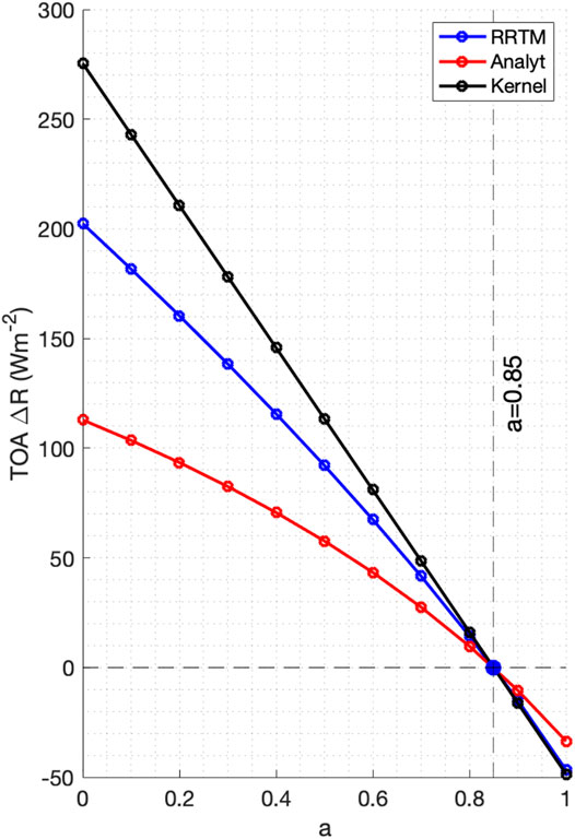
FIGURE 6. All-sky univariate surface albedo SW feedback corresponding to different albedo values. By perturbing the surface albedo to values from 0 to 1, the TOA SW feedback is computed by three different methods: RRTM-computed truth, kernel-estimation and the single-layer analytical model (Eq. 11). The results are compuated based on one arbitrarily chosen grid box at (78°W, 82°N), where the intial surface albedo is 0.85.

Here $r$ and $\tau$ denote atmospheric reflectance and transmittance respectively; they are related as $\tau +r+\epsilon =1$, where $\epsilon$ denotes atmospheric absorptivity. This relation means that $a_p$ and thus the net shortwave radiation flux at TOA has a nonlinear dependency on a:

$\frac{\partial a_p}{\partial a}=\frac{{\tau }^2}{{\left(1-ra\right)}^2}(12)$

That the radiative sensitivity to surface albedo continuously varies with the albedo value makes it difficult for any linear methods such as the kernel method to accurately measure the albedo feedback. It is interesting to notice from Eq. (12) that the radiative sensitivity decreases with a. This means that if the surface albedo kernel is computed with relatively larger albedo values under the unperturbed climate (1xCO₂), it will overestimate the univariate albedo feedback in a warming scenario (4xCO₂). This is clearly seen from Figure 6. If the kernel method is used to estimate the feedback when sea ice completely melts, the intercepts on y-axis indicate the overestimate can be serveral dozens of W m⁻². This overestimation issue was also noted in the previous studies (e.g., Block and Mauristen 2013; Zhu et al., 2019). It is also interesting to notice that although the analytical model qualitatively captures the change of radiative sensitivity to albedo, it does not accurately predict it. The neural network method proposed by Zhu et al. (2019) and Shakirova and Huang (2021) may be better suited for the albedo feedback quantification and deserves further development and more extensive validations.

Multivariate Nonlinear Effects

Besides the univariate nonlinear effects, Eq. (1) indicates that multivariate nonlinear effects, represented by such terms as $\frac{{\partial }^{2}R}{\partial x\partial y}\Delta x\Delta y$, may also strongly contribute to the radiative flux variations. Such terms are often referred to as the coupling effects because they result from concerted variations of the involved variables; otherwise, if their covariance were small, the average of this term over time or region would be negligible. In reality, this necessary condition is usually met because the variations of the feedback variables of concern tend to be strongly correlated. For instance, temperature warming and sea ice melt may expose more open water, which in turn leads to more evaporation, atmospheric humidity and cloudiness.

Due to large computational expenses of the brute-force RTM-based feedback calculation, we base our discussions on two representative months in the 4xCO₂ experiment: January (winter) for the longwave feedbacks and June (summer) for the shortwave feedbacks, because the two types of feedbacks are the most prominent in the two respective seasons. Figures 7,8 show the radiative feedbacks corresponding to the changes in the feedback variables illustrated in Figure 1. Table 1 summarizes their Arctic mean values. These results disclose two strongest multivariate feedback effects in the Arctic: the coupling effect between temperature and cloud, $\Delta R_{tc}$, in the longwave and the coupling effect between albedo and cloud, $\Delta R_{ac}$, in the shortwave.

FIGURE 7

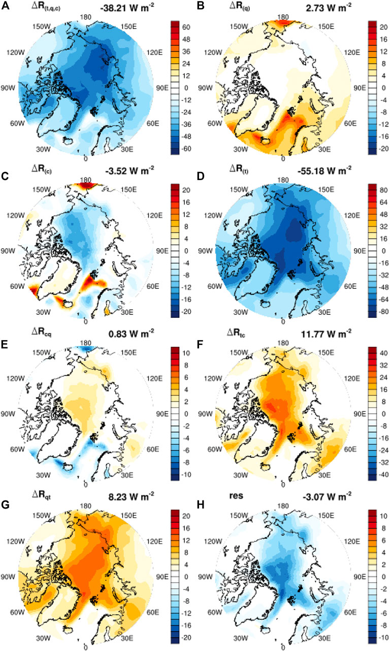
FIGURE 7. All-sky LW feedback effects in January. Units: W m⁻². Shown here are the total and component all-sky feedbacks in the 4xCO₂ experiment evaluated according to Eq. 2, Eq. 3, and Eq. 4 by using an RTM. t: atmospheric and surface temperatures; q: atmospheric water vapor; c: cloud; a: surface albedo; res: residual. The Arctic mean values are noted on the top right corner of each panel.

FIGURE 8

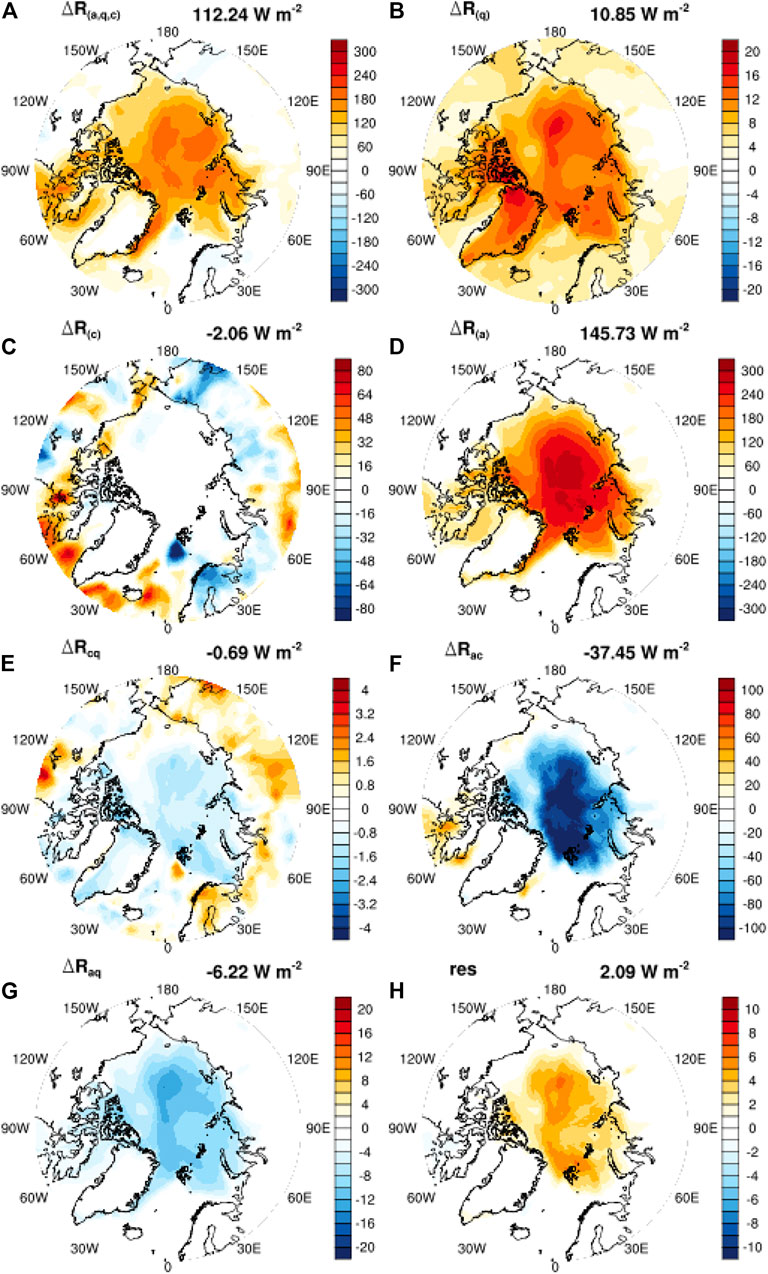
FIGURE 8. Like Figure 7, but for the all-sky SW feedback effects in June. Units: W m⁻².

TABLE 1

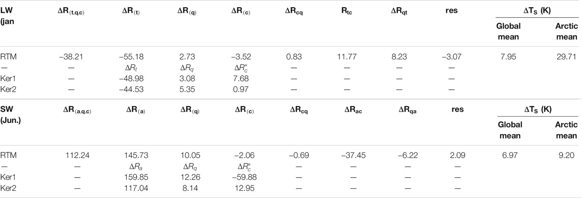
TABLE 1. Arctic mean all-sky feedbacks in the 4xCO2 experiment for the two selected months. Units: W m-2. Area-weighted averages are taken for the region 70–90°N. Two sets of radiative kernels have been used to measure the univariate linear feedbacks: Ker1 is computed from the GCM instantaneous profiles in this work and thus is of no kernel bias; Ker2 is the kernel computed by Huang et al. (2017) from the ERA-interim reanalysis profiles, which leads to biases in diagnosed univariate feedback as explained by Eq. 8.

In the longwave, we find that the multivariate (bivariate) feedback is dominated by the coupling effect between temperature and cloud, $\Delta R_{tc}$. The pattern of this coupling effect resembles, but strongly offsets, the univariate temperature feedback, $\Delta R_{\left(t\right)}$, which is the dominant feedback that controls the overall LW feedback in the Arctic. This coupling effect can be explained by a simple analytical model. Consider a single-layer atmosphere, with temperature $t_a$ and emissivity (absorptivity) $\epsilon$, and assume the surface to be a blackbody with temperature $t_s$:

$OLR=\left(1-\epsilon \right)\sigma t_s^4+\epsilon \sigma t_a^4(13)$

Hence, the coupling effect $\Delta OL{R}_{tc}$ is found to be

$\Delta OL{R}_{tc}=4\sigma \left(t_a^3\text{Δ}{t}_a-t_s^3\text{Δ}{t}_s\right)\frac{d\epsilon }{dc}\Delta c(14)$

Because the warming in the Arctic is capped in near-surface layers, $\text{Δ}{t}_a<<\text{Δ}{t}_s$. This leads to reduction in OLR, offseting the increase of OLR by temperature warming. The coupling effect between temperature and water vapor can be understood in the same way. Becaue water vapor affects OLR also by affecting the atmospheric emissivity; the coupling effect $\Delta OL{R}_{tq}$ is thus also affected by the factor $(t_a^3\text{Δ}{t}_a-t_s^3\text{Δ}{t}_s)$ in Eq. (14). Although this nonlinear effect arises from the nonuniform vertical structure of temperatuure warming and thus share the physical cause of the temperature lapse rate feedback, this nonlinear effect should be distinguished from the lapse rate feedback, which is part of the univariate temperature feedback, $\Delta R_t$. Note that the sign of $\Delta R_{tc}$ and $\Delta R_{cq}$ is positive in Figure 7 because the fluxes are defined to be downward positive.

In the shortwave, the dominant multivariate effect is found to be the albedo-cloud coupling, which offsets the univariate albedo feedback. From the simple model described above (Eq. 11 and Eq. 12, this can be understood as cloud-caused reduction in the atmospheric transmittance and thus reduction in the radiative senstivity to surface albedo.

It is interesting to note that the patterns of some coupling feedback effects are correlated with the change patterns of the associated feedback variables. For example, the LW cloud-temperature coupling effect is correlated with surface temperature change, with a correlation coefficient of 0.86; the LW cloud-water vapor coupling effect is correlated with total water vapor (TCWV) at 0.62; the SW albedo-cloud coupling effect is correlated with the surface albedo change at 0.89. Such relation suggests that it may be possible to estimate these nonlinear effects using analytical or statistical models. Huang and Huang (2021) used such an model to explain the cloud-water vapor coupling effect and found it to be the dominant multivariate longwave feedback effect in the tropics. Although this coupling effect is not as strong compared to the temperature-related coupling effects in the Arctic, we find that adopting the same estimation method of Huang and Huang, 2021, Eq. 19 and using a parameter value appropriate to the Arctic (A = 0.04 kg⁻¹ m²), we can very well predict the cloud-water vapor coupling effect (spatial correlation = 0.99, RMSE = 0.41 W m⁻²). Future works are warranted to identify methods for explaining and predicting the other coupling effects.

Lastly, for comparison, we include in Table 1 the respective feedbacks analyzed from the kernel method, i.e., the univariate linear effects for non-cloud feedbacks and the cloud feedback ($\Delta R_c^{\ast }$) obtained as a residual of total radiation change decomposition. Besides the biases in the univariate feedbacks as noted above, it is worth noting that the kernel-based estimations may also greatly bias the cloud feedback, mainly due to its negligence of the coupling effects.

Conclusions and Discussions

In this paper, we present an overview of the nonlinear effects in both longwave and shortwave radiative feedbacks in the CO₂-driven Arctic warming. Based on brute-force radiation model calculations we disclose the most prominent nonlinear feedback effects and based on simple analytical models we offer explanations of their physcial causes. Although the presentation and discussion are focused on the Arctic feedbacks, the diagnostic framework (Eq. 1) and the theoretical explanations are applicable to global feedback analyses.

We identify these important nonlinear feedback effects:

1) The univariate nonlinear effect in the surface albedo feedback in the shortwave. This nonlinearity can be understood from a simple analytical model [Eq. (11)] that accounts for the coupling, due to multiple-scattering, between the surface and atmosphere (clouds). This coupling makes the radiative sensitivity to surface albedo decrease with the surface albedo value (Figure 6). Because of this effect, it generally leads to an overestimate of the surface albedo feedback when albedo kernels computed from the current climate are used to quantify the albedo feedback in a warming climate (Figure 3; Table 1).

2) The bivariate surface albedo-cloud coupling effect in the shortwave. This effect is attributable to the masking effect of cloud increase that damps the radiative sensitivity to surface albedo. This effect is the most prominent in the summer when solar insolation is strong, as illustrated by Figure 8 for the month of June.

3) The multivariate temperature-cloud feedback in the longwave. This effect is attributable to the fact that the Arctic warming is much stronger at and near the surface than in the upper air, which leads to a damping effect on the temperature feedback. This nonlinear effect should be distinguished from the temperature lapse rate feedback and is found to be the strongest in the winter as illustrated by Figure 7 for the month of January.

4) Although the univariate water vapor feedback largely scales logarithmically with water vapor changes, it is found that the relation deviates from the logarithmic scaling, especially in the window band. This is due to the unsaturated atmospheric absorption in this band and suggests that a hybrid scaling method as proposed by Eq. (10) may improve the accuracy of the kernel-diagnosed water vapor feedback (compare Figure 2C and Figure 5C).

It should be noted that the large nonlinear effects discovered here is not limited to the 4xCO₂ experiment. As shown by Huang and Huang (2021) for the longwave feedbacks and Shakirova and Huang (2021) for the shortwave feedbacks, similar, strong nonlinear effects exist even also interannual climate variations. It is noted that the nonlinear effects may quantitatively differ in different forcing experiments, thus requiring them to be assessed more comprehensively in future work.

The strong nonlinear effects as disclosed here call into question the accuracy of linear methods currently used in the feedback analysis. Nonlinear methods are needed to improve the accuracy of feedback quantificaiton when RTM-based PRP experiments are not feasible due to its forbidding computational demands. Especially in need are replacement of the linear kernels for the surface albedo feedback and cloud feedback quantification. Although a handful of studies have touched this topic, for instance, using quadratic fitting (Colman et al., 1997), histogram (Zelinka et al., 2012) and neural network (Zhu et al., 2019) methods, this challenging problem demands devoted research programs to further develop, test and mature the candidate methods.

Data Availability Statement

The datasets presented in this study can be found in online repositories. The names of the repository/repositories and accession number(s) can be found below: The CESM codes can be downloaded from National Center for Atmospheric Research (NCAR) website (http://www.cesm.ucar.edu/models/cesm1.2/). The RRTM code can be downloaded at http://rtweb.aer.com/rrtm_frame.html.

Author Contributions

YH designed the research and wrote the paper. HH conducted the longwave feedback analysis and AS conducted the shortwave feedback analysis.

Conflict of Interest

The authors declare that the research was conducted in the absence of any commercial or financial relationships that could be construed as a potential conflict of interest.

Publisher’s Note

All claims expressed in this article are solely those of the authors and do not necessarily represent those of their affiliated organizations, or those of the publisher, the editors and the reviewers. Any product that may be evaluated in this article, or claim that may be made by its manufacturer, is not guaranteed or endorsed by the publisher.

Acknowledgments

We thank Tim Merlis, Ivy Tan, Patrick Taylor and two reviewers, whose comments helped improve this paper. We acknowledge grants from the Natural Sciences and Engineering Research Council of Canada (RGPIN-2019-04511) and from the Fonds de recherche du Québec—Nature et technologies (2021-PR-283823).

References

Bani Shahabadi, M., and Huang, Y. (2014). Logarithmic Radiative Effect of Water Vapor and Spectral Kernels. J. Geophys. Res. Atmos. 119 (10), 6000–6008. doi:10.1002/2014jd021623

CrossRef Full Text | Google Scholar

Block, K., and Mauritsen, T. (2013). Forcing and Feedback in the MPI-ESM-LR Coupled Model under Abruptly Quadrupled CO2. J. Adv. Model. Earth Syst. 5 (4), 676–691. doi:10.1002/jame.20041

CrossRef Full Text | Google Scholar

Colman, R. A., Power, S. B., and McAvaney, B. J. (1997). Non-linear Climate Feedback Analysis in an Atmospheric General Circulation Model. Clim. Dyn. 13 (10), 717–731. doi:10.1007/s003820050193

CrossRef Full Text | Google Scholar

Colman, R., and McAvaney, B. J. (1997). A Study of General Circulation Model Climate Feedbacks Determined from Perturbed SST Experiments. J. Geophys. Res. 102, 19 383–419. doi:10.1029/97jd00206

CrossRef Full Text | Google Scholar

Huang, H., and Huang, Y. (2021). Nonlinear Coupling between Longwave Radiative Climate Feedbacks. J. Geophys. Res.

CrossRef Full Text | Google Scholar

Huang, Y. (2013). On the Longwave Climate Feedbacks. J. Clim. 26 (19), 7603–7610. doi:10.1175/jcli-d-13-00025.1

CrossRef Full Text | Google Scholar

Huang, Y., Ramaswamy, V., and Soden, B. (2007). An Investigation of the Sensitivity of the clear‐sky Outgoing Longwave Radiation to Atmospheric Temperature and Water Vapor. J. Geophys. Res. Atmospheres 112 (D5). doi:10.1029/2005jd006906

CrossRef Full Text | Google Scholar

Huang, Y., Xia, Y., and Tan, X. (2017). On the Pattern of CO2 Radiative Forcing and Poleward Energy Transport. J. Geophys. Res. Atmos. 122 (10), 578–593. doi:10.1002/2017jd027221

CrossRef Full Text | Google Scholar

Mlawer, E. J., Taubman, S. J., Brown, P. D., Iacono, M. J., and Clough, S. A. (1997). Radiative Transfer for Inhomogeneous Atmospheres: RRTM, a Validated Correlated-K Model for the Longwave. J. Geophys. Res. 102 (D14), 16663–16682. doi:10.1029/97jd00237

CrossRef Full Text | Google Scholar

Sanderson, B. M., and Shell, K. M. (2012). Model-Specific Radiative Kernels for Calculating Cloud and Noncloud Climate Feedbacks. J. Clim. 25 (21), 7607–7624. doi:10.1175/jcli-d-11-00726.1

CrossRef Full Text | Google Scholar

Shakirova, A., and Huang, Y. (2021). An Neural Network Model for Shortwave Radiative Feedback Estimation. J. Geophys. Res. Atmosphere under revision for.

Google Scholar

Shell, K. M., Kiehl, J. T., and Shields, C. A. (2008). Using the Radiative Kernel Technique to Calculate Climate Feedbacks in NCAR's Community Atmospheric Model. J. Clim. 21 (10), 2269–2282. doi:10.1175/2007jcli2044.1

CrossRef Full Text | Google Scholar

Smith, C. J., Kramer, R. J., and Sima, A. (2020). The HadGEM3-GA7.1 Radiative Kernel: the Importance of a Well-Resolved Stratosphere. Earth Syst. Sci. Data Discuss 12, 2057–2068. doi:10.5194/essd-2019-254

CrossRef Full Text | Google Scholar

Soden, B. J., and Held, I. M. (2006). An Assessment of Climate Feedbacks in Coupled Ocean-Atmosphere Models. J. Clim. 19 (14), 3354–3360. doi:10.1175/jcli3799.1

CrossRef Full Text | Google Scholar

Soden, B. J., Held, I. M., Colman, R., Shell, K. M., Kiehl, J. T., and Shields, C. A. (2008). Quantifying Climate Feedbacks Using Radiative Kernels. J. Clim. 21 (14), 3504–3520. doi:10.1175/2007jcli2110.1

CrossRef Full Text | Google Scholar

Vial, J., Dufresne, J.-L., and Bony, S. (2013). On the Interpretation of Inter-model Spread in CMIP5 Climate Sensitivity Estimates. Clim. Dyn. 41 (11-12), 3339–3362. doi:10.1007/s00382-013-1725-9

CrossRef Full Text | Google Scholar

Wang, Y., and Huang, Y. (2020). The Surface Warming Attributable to Stratospheric Water Vapor in CO2‐caused Global Warming. J. Geophys. Res. Atmospheres 125, e2020JD032752. doi:10.1029/2020JD032752

CrossRef Full Text | Google Scholar

Wetherald, R. T., and Manabe, S. (1988). Cloud Feedback Processes in a General Circulation Model. J. Atmos. Sci. 45 (8), 1397–1416. doi:10.1175/1520-0469(1988)045<1397:cfpiag>2.0.co;2

CrossRef Full Text | Google Scholar

Yue, Q., Kahn, B. H., Fetzer, E. J., Schreier, M., Wong, S., Chen, X., et al. (2016). Observation-Based Longwave Cloud Radiative Kernels Derived from the A-Train. J. Clim. 29, 2023–2040. doi:10.1175/JCLI-D-15-0257.1

CrossRef Full Text | Google Scholar

Zelinka, M. D., Klein, S. A., and Hartmann, D. L. (2012). Computing and Partitioning Cloud Feedbacks Using Cloud Property Histograms. Part I: Cloud Radiative Kernels. J. Clim. 25 (11), 3715–3735. doi:10.1175/jcli-d-11-00248.1

CrossRef Full Text | Google Scholar

Zhang, M. H., Hack, J. J., Kiehl, J. T., and Cess, R. D. (1994). Diagnostic Study of Climate Feedback Processes in Atmospheric General Circulation Models. J. Geophys. Res. 99 (D3), 5525–5537. doi:10.1029/93jd03523

CrossRef Full Text | Google Scholar

Zhang, M., and Huang, Y. (2014). Radiative Forcing of Quadrupling CO2. J. Clim. 27 (7), 2496–2508. doi:10.1175/jcli-d-13-00535.1

CrossRef Full Text | Google Scholar

Zhu, T., Huang, Y., and Wei, H. (2019). Estimating Climate Feedbacks Using a Neural Network. J. Geophys. Res. Atmos. 124 (6), 3246–3258. doi:10.1029/2018jd029223

CrossRef Full Text | Google Scholar