Exploring the Adequacy of Steady-State-Only Calibration

This paper explores the adequacy of steady-state-only calibration as a precursor to use of a groundwater model for decision-support. First, it reviews metrics by which a decision-support model should be judged. On the basis of these metrics, it establishes the shortcomings that a decision-support model may incur through foregoing transient calibration. These are 1) failure to reduce the uncertainties of management-salient model predictions to the extent that available data allows, and 2) creation of unquantifiable bias in management-salient predictions. Two methodologies for quantification of these deficiencies are proposed. The first of these addresses uncertainty reduction. This is relatively easy to implement, as it requires only that sensitivities of pertinent model outputs to a model’s parameters be calculated. The second methodology addresses predictive bias. Implementation of this second methodology is more expensive as it requires repeated calibration of a steady state model against stochastic realizations of a transient model.These methods are demonstrated using a synthetic case which explores the viability of steady-state-only calibration of models deployed to examine the impacts of pumping on stream flows and groundwater levels. It is demonstrated that, for some predictions of management interest, steady-state-only calibration is more than sufficient for this kind of decision-support modelling.

Introduction

In this paper we address the utility of steady state model calibration. In particular, we inquire whether a model that has undergone only steady state calibration can provide a basis for decision support, especially in contexts where some management-salient predictions are transient in nature.

Often, in courtrooms and in other forums of public debate, a steady state model is susceptible to challenge. An opposing party may argue that groundwater processes are never steady state, and that the role of simulation is to replicate real-world processes on a computer. It follows that a simulator must prove its worth by reproducing the full historical behaviour of a natural system, and not some abstract artifact such as “average behaviour”. Unless it can do this, its decision-support role is questionable at best and invalidated at worst.

This argument is, of course, too simplistic. However, this does not prevent its repetition, nor its ability to influence the perceptions of those who are unfamiliar with modelling concepts. At the same time, its refutation in the court of public opinion is not easy. Part of the reason for this is that the metrics by which decision-support modelling should be judged are not clear—even to many in the groundwater industry. Even if they were made clear, and were commonly accepted, assessment of a particular modelling strategy according to appropriate metrics may not be a straightforward matter.

The purpose of this paper is to state decision-support metrics, and to present an example of how steady-state-only model calibration can be assessed using these metrics. However, before doing this, it is salient to consider some of the problems that beset calibration of a transient model, and the assumptions and abstractions on which transient simulation rests.

Transient recharge processes are complex. The processes which prevail during moderate rain events may differ greatly from those that prevail during times of heavy rainfall. During a significant rain event, shallow saturation, and fast vertical flow through macropores, can deliver water rapidly to an aquifer. Meanwhile, surficial ponding of water and overbank flow of streams can enhance and concentrate recharge at other locations. Nor is simulation of groundwater recharge processes straightforward in drier times. If unsaturated drainage of water through a vertical soil column at the representative elementary volume scale can be described by Richard’s equation, it does not follow that this same equation describes spatially-averaged drainage over the many heterogeneous soil columns which collectively fill a single groundwater model cell (Farthing and Ogden, 2017). Complications are increased where irrigation supplements rainfall, and where groundwater recharge experiences significant delays as it travels through the unsaturated zone (Healy and Scanlon, 2010; Hocking and Kelly, 2016). All of these processes are difficult to simulate.

Simulation of the transient behaviour of groundwater is also beset with difficulties. Transient groundwater models take longer to build and run than steady state models. Their numerical stability may be compromised as a fluctuating water table traverses multiple layers of a model. These factors render computer-aided calibration and uncertainty analysis much more difficult than for steady state models.

While the information content of transient water levels and fluxes is higher than that of their static counterparts, this information must inform many more parameters when history-matching (also referred to as calibration or data assimilation) is undertaken under transient conditions. The additional parameters that must be informed through history-matching of a transient model include those that describe groundwater storage, as well as those that describe partitioning of rainfall and irrigation between recharge, runoff and evapotranspiration in the unsaturated zone. Nevertheless, if model predictions of management interest are similar in nature to those that comprise a transient calibration dataset, then assimilation of this information can indeed reduce the uncertainties of these predictions. This reduction occurs even if individual model parameters remain nonunique, and even if some of them must adopt roles which compensate for abstract representations of the real world in a numerical simulator (Schilling et al., 2014; Doherty, 2015).

In other cases, the uncertainties of predictions made by a transient model may be reduced very little, if at all by history-matching. This is the case if the conditions under which predictions of future system behaviour are required are very different from those which prevailed in the past. Under these conditions, it is not impossible for history-matching to achieve good replication of historical transient system behaviour while introducing unquantifiable bias to predictions of future transient behaviour, especially those pertaining to extremely wet and extremely dry conditions (Doherty and Christensen, 2011; White et al., 2014; Knowling et al., 2020a).

In contrast to transient models, steady state models generally run quickly. They are much more easily subjected to computer-aided history-matching and uncertainty analysis. At the same time, reliable estimates of long-term recharge to use in these models can often be obtained through techniques such as chloride balance (Shaw and Thorburn, 1985; Wood, 1999; Crosbie et al., 2017). Furthermore, an inversion process based on steady-state-only history-matching can focus on estimation of conductance parameters while avoiding the simultaneous estimation of parameters which affect transient groundwater behaviour. It is these conductance parameters that determine the final state of a system when it is subjected to long-term stresses which are significantly different from those which it has experienced in the past.

Decision Support Metrics

Metrics through which the efficacy of decision-support modelling can be assessed were presented by Freeze et al. (1990). Use of these metrics in assessing model simplification strategies has been discussed by Doherty and Simmons (2013), and more recently by Doherty and Moore (2019). These metrics are based on the premise that predictions made by a groundwater model are uncertain. Uncertainties arise from the complex and heterogenous processes that affect groundwater recharge and movement through the subsurface, coupled with a deficit of data that have the potential to inform the properties which govern these processes. A high degree of non-uniqueness (sometimes referred to as equifinality) therefore accompanies the parameterization of a groundwater model. Parameter non-uniqueness induces a high degree of uncertainty in some model predictions, particularly those which describe a groundwater system’s response to new stresses.

Ideally, modelling serves the decision-making process by sampling the posterior probability distributions of predictions of management interest (Knowling et al., 2020b; White et al., 2020). Here we use “posterior” in the Bayesian sense. Bayes equation states that assimilation of information that is resident in the historical behaviour of a system reduces uncertainties associated with predictions of its future behaviour below those which they would possess if informed by expert knowledge alone. When predictions of future system behaviour are accompanied by assessments of their uncertainties, decision-makers are acquainted with the risks associated with contemplated management strategies.

In practice, characterization of the entire posterior probability distribution of a prediction of management interest may be neither possible nor necessary. Taking this into account, the primary requirements of effective decision-support modelling are now listed.

• The decision-support modelling process should provide at least an approximate characterization of the uncertainties of decision-critical model predictions, particularly as these pertain to unwanted aspects of system behaviour.

• Because estimates of posterior uncertainty are themselves uncertain, they should err on the conservative side so that risks are overestimated rather than underestimated.

• Where choices between different management options are difficult to make, and where risks are high, the decision-support modelling process should reduce predictive uncertainties as much as possible through data assimilation; this can be achieved through computer-aided history-matching.

Application to Steady State Modelling

We now apply these metrics to a context in which a numerical model is run under steady state conditions for the purpose of history-matching but may be deployed to make predictions which are transient in nature. Obviously, some of the model’s parameters to which management-salient predictions are sensitive are not informed by the past transient behaviour of the system when the model undergoes steady-state-only calibration. Knowledge of these uninformed parameters must therefore be based on local expertise and site characterization.

Steady-state-only history-matching impacts the ability of decision-support modelling to satisfy the above-listed metrics in three distinct ways. To simplify the following discussion, we categorize these impacts as type 1, 2 and 3 in order to conform with the convention adopted by Nicol and Doherty (2021) to describe shortcomings induced by use of a simple model in place of a more complex one. These are now described. Figure 1 depicts the conceptual workflow adopted for analysing these shortcomings in our study. The steps that comprise this workflow are applicable to more general analyses of decision-support model appropriateness.

FIGURE 1

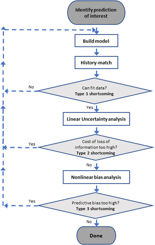
FIGURE 1. Flow chart for examining shortcomings in model design.

Type 1 Shortcomings

A simplified model may not be able to replicate past system behaviour as well as a more complex model. This may lead to high levels of model-to-measurement misfit as it is calibrated. History-matching therefore fails to assimilate all of the information that is resident in measurements of historical system behaviour. The uncertainties of decision-critical model predictions may not therefore be reduced to levels that are commensurate with this information, as the model does not hold enough parameters to provide receptacles for it. The information that is denied entry to the model expresses itself as so-called “structural noise”. This manifests itself as model-to-measurement misfit which bears significant spatial and/or temporal correlation.

Because the principal agent of model-to-measurement misfit under these circumstances is model structural inadequacies rather than random measurement error, its effect on posterior parameter and predictive uncertainties is difficult to characterize. Nevertheless, methods have been proposed that can accommodate, to some extent, parameter and predictive uncertainties forthcoming from model inadequacies. See, for example, Kennedy and O’Hagan (2001), Cooley and Christensen (2006) and Oliver and Alfonzo (2018).

We refer to modelling shortcomings arising from this source as type 1 shortcomings. They are often of secondary concern in steady state model calibration. This is because it is generally possible to attain a good fit between model outputs and (processed) field measurements that comprise a steady state calibration dataset in a highly-parameterized, regularized inversion setting. If a good fit cannot be achieved, this is normally indicative of severe conceptual and structural model inadequacies as discussed in the paragraph above. Once these have been exposed by the steady state history-matching process, they can be rectified.

Type 2 Shortcomings

In the present context, we classify type 2 shortcomings as those that arise from the impaired capacity of steady-state-only model calibration to reduce the posterior uncertainties of predictions of future transient groundwater behaviour. When a model undergoes steady-state-only calibration, the history-matching process is not given access to information that has the capacity to reduce some of these uncertainties. Inflated uncertainties may render the choice between one management strategy and another more difficult.

Fortunately, as is demonstrated below, the decision-support repercussions of type 2 shortcomings are relatively easy to assess through linear analysis (Doherty, 2015). Based on information forthcoming from this analysis, modellers, and modelling stakeholders, can decide whether the benefits of transient calibration are worth the cost in their particular management context.

Type 3 Shortcomings

Despite achieving a good fit with field measurements, a simplified model may not represent all processes and/or parameters that affect these measurements. Fitting them with abbreviated processes/parameters may introduce parametric and predictive bias. We denote calibration-induced bias as type 3 shortcomings herein. This is much more difficult to recognize and quantify than the other two types of shortcomings.

In the context of the present discussion, type 3 shortcomings arise from the fact that the “steady state” condition is a conceptual artifact. As groundwater levels rise and fall with season, the direction of groundwater flow may change as discharge locations shift. Selection of a time, or averaging process, that can be decreed as “steady state” may be questionable if recharge and discharge processes are nonlinear (as they usually are). Consequently, the assumption that temporally-averaged borehole water levels comprise a system’s response to temporally-averaged recharge may be questionable. Alternatively, a modeller may assume that borehole heads that prevailed over a time period when they were relatively static can be considered to be steady state for the purpose of model calibration; however, the groundwater recharge that prevailed over this time may be difficult to quantify.

Conceptually, uncertainties in “steady state recharge” and in “steady state heads” can be acknowledged by ascribing appropriate uncertainties to these quantities when undertaking computer-based data assimilation. These uncertainties are then propagated to model parameters, and thereby to model predictions. However, head and recharge uncertainties that describe departures from the steady state assumption are likely to exhibit high degrees of spatial correlation. In practice, their uncertainties will be very difficult to characterize.

Means through which parameter and predictive biases incurred by history-matching of a defective model can be characterized are described by Doherty and Christensen (2011) and White et al. (2014). We briefly discuss the latter method first.

White et al. (2014) demonstrate that, for the purpose of analysing calibration-induced predictive bias, the relationship between a simple model and a “correct” model is that the former can be derived from the latter by fixing certain of its parameters at incorrect values. As noted above, this may not impair the ability of the history-matching process to attain a good fit between simple model outputs and field measurements, especially in highly parameterized contexts. However, in attaining this fit, estimated parameters of the simple model may adopt roles which compensate for its defects. To the extent that decision-critical model predictions are sensitive to either the defect parameters, and/or to the parameters that compensate for these defects as the model is calibrated, they may inherit bias. In theory, this bias can be quantified using linear analysis. In practice this procedure is difficult to implement when exploring the repercussions of steady-state-only model calibration as “defect parameters” cannot be readily defined in this context.

In contrast, the methodology proposed by Doherty and Christensen (2011) to explore the impacts of model defects on post-history-matching predictive bias does not require identification of “defect parameters”. However, implementation of this method requires much greater numerical effort. It also requires definition of a “correct” model and a complementary simple model. The propensity for predictive bias can be evaluated through paired-model analysis. We base our analysis of type 3 shortcomings arising from steady-state-only calibration on this methodology.

Methodology

Details of analyses used for exploration of drawbacks incurred by steady-state-only calibration are now provided. We do not address type 1 shortcomings herein as we assume that parameters of a steady state model can be adjusted in order for its outputs to provide a satisfactory fit with a steady state calibration dataset.

Analysis of Type 2 Shortcomings

If the action of a model on its parameters is approximated by the action of a matrix on a vector, its action during the calibration process can be described by the following equation.

$\mathbf{h}=\mathbf{Zk}+\mathbf{\epsilon }(1)$

In Equation 1, the vector h denotes observations comprising a calibration dataset, while the vector k denotes model parameters. The vector ε expresses noise associated with the measurement dataset. Each column of the matrix Z is comprised of sensitivities of a calibration-relevant model output to a single parameter (Z is also often referred to as the Jacobian matrix).

Let C(k) denote the prior covariance matrix of model parameters. The diagonal elements of this matrix represent the squares of prior parameter standard deviations, i.e. the uncertainties of model parameters when the latter are informed by expert knowledge alone. Off-diagonal elements of C(k) reflect prior parameter correlation. For spatial parameters such as hydraulic conductivity, spatial correlation reflects a tendency for above- and below-average values of this hydraulic property to exhibit spatial continuity.

Let C(ε) (another covariance matrix) denote the statistical properties of whatever is responsible for model-to-measurement misfit. When calibrating a steady state model, C(ε) receives contributions from errors in field measurements, as well as from errors in the assumption that a particular field measurement represents a steady state condition. For convenience, this matrix is often assumed to be diagonal, this implying that measurement errors are independent of each other (a tenuous assumption when its relationship to model structural and conceptual imperfections is recognized). The magnitudes of the elements of C(ε) dictate the level of model-to-measurement fit that should be pursued through history-matching.

Suppose that the model makes a prediction. We denote it as s (a scalar). Its action in making this prediction can be characterized by the equation:

$s={\mathbf{y}}^{\mathbf{t}}\mathbf{k}(2)$

In this equation, the elements of the vector y are sensitivities of the prediction s to each of the elements of k. Let us characterize the post-calibration variance of s by the symbol σ²_s. (Variance is the square of standard deviation.) In a linear world, the variance of prior uncertainty of s can be computed using the following matrix equation.

${\text{σ}}_{\text{s}}^2={\mathbf{y}}^{\mathbf{t}}\text{C}\left(\mathbf{k}\right)\mathbf{y}(3)$

Meanwhile, the variance of posterior predictive uncertainty can be computed using either of the following two equivalent matrix equations.

${\text{σ}}_{\text{s}}^2={\mathbf{y}}^{\mathbf{t}}\text{C}\left(\mathbf{k}\right)\mathbf{y}-{\mathbf{y}}^{\mathbf{t}}\text{C}\left(\mathbf{k}\right){\mathbf{Z}}^{\mathbf{t}}{\left[\mathbf{Z}\text{C}\left(\mathbf{k}\right){\mathbf{Z}}^{\mathbf{t}}+\text{C}\left(\mathbf{\epsilon }\right)\right]}^{-1}\mathbf{Z}\text{C}\left(\mathbf{k}\right){\mathbf{y}}^{\mathbf{t}}(4)$

${\text{σ}}_{\text{s}}^2={\mathbf{y}}^{\mathbf{t}}{\left[{\mathbf{Z}}^{\mathbf{t}}{\text{C}}^{-1}\left(\mathbf{\epsilon }\right)\mathbf{Z}+{\text{C}}^{-1}\left(\mathbf{k}\right)\right]}^{-1}\mathbf{y}(5)$

Equation 4 is particularly revealing. The second term of this equation quantifies the extent to which history-matching reduces the uncertainty variance of s. See Doherty (2015) for further details.

Use of the above equations requires that a modeller fill the Z matrix and y vector with model-output-to-parameter sensitivities. This can normally be done by running the model repeatedly with each of its parameters in turn varied incrementally from a reference value. Model outputs are divided by parameter differences to obtain sensitivities.

It is important to note that when undertaking linear uncertainty analysis, the reference parameter fields on which finite-difference model runs are based do not need to express heterogeneity that is embodied in C(k); in fact, these parameter fields can be homogeneous. The effect of parameter heterogeneity on predictive uncertainty is expressed solely through Equations 3, 4 and 5. It is also important to note that these equations do not include k. Nor do they include the observation vector h nor the prediction s. This has an important repercussion. It means that the ability of a history-matching process to reduce the uncertainty of a prediction of interest can be gauged without actually gathering the data that comprises the history-matching dataset, nor actually subjecting the model to history-matching. The above equations require only the sensitivities of model outputs that would be matched to a notional calibration dataset. The calibration dataset does not have to actually exist. (We note, however, that model nonlinearities are best accommodated by evaluating sensitivities using calibrated parameter values.)

Assessment of type 2 shortcomings that beset steady-state-only calibration is therefore a relatively simple matter. It requires only that the following steps be undertaken.

1. Construct a transient model to run over an historical time period, and then over a predictive time period.

2. Identify measurements comprising a transient history-matching dataset. As stated above, these measurements may have been taken only in our imagination.

3. Build a representative C(ε) matrix on the basis of likely misfits between model outputs and respective members of the history-matching dataset.

4. Build a parameter covariance matrix C(k) based on experience, and knowledge of the area that the model represents. Construction of this matrix is normally based on one or a number of variograms. Utility software from the PEST (Doherty, 2020) and PyEMU (White et al., 2016) suites can be used for this task.

5. Populate the Z and y matrices of Equations 4, 5 through repeated model runs based on finite parameter differences.

6. Compute the posterior uncertainty of a prediction s, or of a number of predictions of interest, using Equation 4 or 5.

7. Configure the model to run under steady state conditions; specify a notional steady state calibration dataset.

8. Build a C(ε) matrix for this steady state calibration dataset, this reflecting the fit that the modeller expects to attain with it.

9. Populate the steady state Z and y matrices through repeated model runs based on finite parameter differences.

10. Compute the posterior uncertainty of s again using Equation 4 or 5 on the basis of steady-state-only calibration. Presumably this uncertainty will be greater than that calculated under the presumption of transient calibration.

11. The difference between these two posterior uncertainties quantifies type 2 shortcomings as they pertain to steady-state-only calibration.

Analysis of Type 3 Shortcomings

As stated above, we employ the method developed by Doherty and Christensen (2011) for exploration of predictive bias incurred through steady-state-only calibration. Steps are as follows; see the above publication for theory.

1. Populate a transient model with a suite of random parameter fields sampled from the prior parameter probability distribution, of which C(k) is the covariance matrix.

2. Run the transient model under both calibration and predictive conditions using each of these parameter fields. For a prediction s, model outputs obtained in this way constitute samples of its prior probability distribution. We denote the value of this prediction as calculated using the i’th random parameter set as s_i.

3. Formulate a steady state history-matching dataset for each random parameter set, using transient heads and fluxes computed by the model at steady state measurement locations. Steady state measurements can generally be computed from transient model outputs by temporal averaging.

4. Populate a C(ε) matrix to characterize steady state history-matching. Calculate a target least-squares objective function that reflects this C(ε).

5. For each parameter set i, calibrate a steady state version of the model against the steady state calibration dataset obtained from the transient model. Employ Tikhonov regularization as described by Doherty (2003) to ensure that the objective function is not less than the target.

6. For each parameter set i, make the model prediction s_i using steady-state-calibrated parameter values when making transient predictions; use prior mean values for storage parameters that were not estimated through steady state calibration.

7. Create a scatter plot in which the s_i prediction made by the transient model is plotted on the y axis while the s_i prediction made by the complementary steady-state-calibrated model is plotted on the x axis for all i.

Doherty and Christensen (2011) explain how an “s vs s” plot obtained in this manner should be interpreted. Refer to Figure 2. The total vertical scatter of s measures the prior uncertainty of this prediction. Meanwhile, points in the scatter plot should ideally be disposed symmetrically about a line whose slope is unity. To the extent that parameters must adopt roles that compensate for model defects in order to fit the calibration dataset, the s vs s scatter plot endures a sideways shift. Often this shift is parameter-dependent and results in a best-fit slope of less than unity. This shift is a measure of predictive bias; as such, it specifies the magnitude of type 3 shortcomings as it pertains to the prediction. Meanwhile, the vertical scatter about the line of best fit is indicative of the posterior uncertainty of the prediction; because the model is nonlinear, this can vary with the value of the prediction.

FIGURE 2

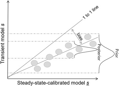
FIGURE 2. Comparison of predictions made by transient models and complimentary steady state models.

Obviously, this process is numerically intensive. However, the numerical burden is somewhat mitigated if the steady state model runs quickly.

A Synthetic Case Study

General

We now apply these methodologies to a simple synthetic case. The issue that is addressed in this example is the effect of groundwater extraction on groundwater levels and stream flows, particularly on low stream flows. We identify a number of management-pertinent predictions that are required of the modelling process. Some of these are time-averaged quantities that characterize the long-term effects of groundwater extraction on a stream. Other predictions, though long term, have transient overtones, in particular the fraction of time over which flow in the stream is below a certain threshold.

In this example, subsurface properties, stream flows, rainfall and potential evaporation rates reflect those encountered in many New Zealand studies that have been undertaken to explore this issue (see, for example, Knowling et al., 2019; White et al., 2019; Hemmings et al., 2020). The authors do not claim that conclusions drawn from this single study can be applied in all management contexts. However, the methodologies that are outlined herein are generally applicable.

Figure 3A shows the rectangular domain of a synthetic model whose dimensions are 7 km by 12 km. The model includes a single layer which represents an unconfined aquifer. The land surface is planar and slopes to the south west; highest and lowest elevations are 11.96 and 0.05 m respectively. A perennial stream flows along the bottom of the model domain. Its bed is incised 6 m into the land surface; this is referred to as “reach 1” in the discussion that follows. Another stream, referred to as “reach 2”, flows down the western border of the model domain. Its incision varies between 5 m at its southern end where it joins the larger stream, and 0 m at a distance of 6 km upstream. All other model boundaries are of the no-flow type.

FIGURE 3

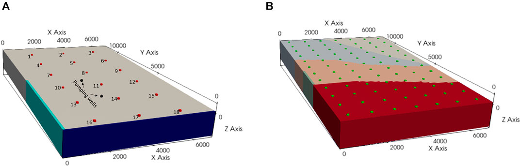
FIGURE 3. Rectangular domain of the synthetic model. (A) Reach 1 runs along the bottom of the model domain (dark blue) and reach 2 runs along the side of the model domain (turquoise). Observation wells are depicted as red circles, and the two pumping wells are depicted as black circles. (B) Spatial distribution of soils across the model domain; brown soils are red, pallic soils are pink, and the two moderate soils are blue (moderate 1) and green (moderate 2). Pilot point locations are depicted as green circles.

Flow of water within the model domain is simulated using MODFLOW-NWT (Niswonger et al., 2011) based on a uniform grid whose cells are 100 m by 100 m. Its streamflow routing (SFR) package simulates stream flow and inflow of groundwater to reaches 1 and 2. Figure 4A shows flow of water into the upstream end of reach 1 over a 9 year period, this being the model’s simulation time; there is no external inflow to reach 2. Water level variations within reach 1 induced by variations in streamflow span a range of about 2.8 m during the 9 year simulation time.

FIGURE 4

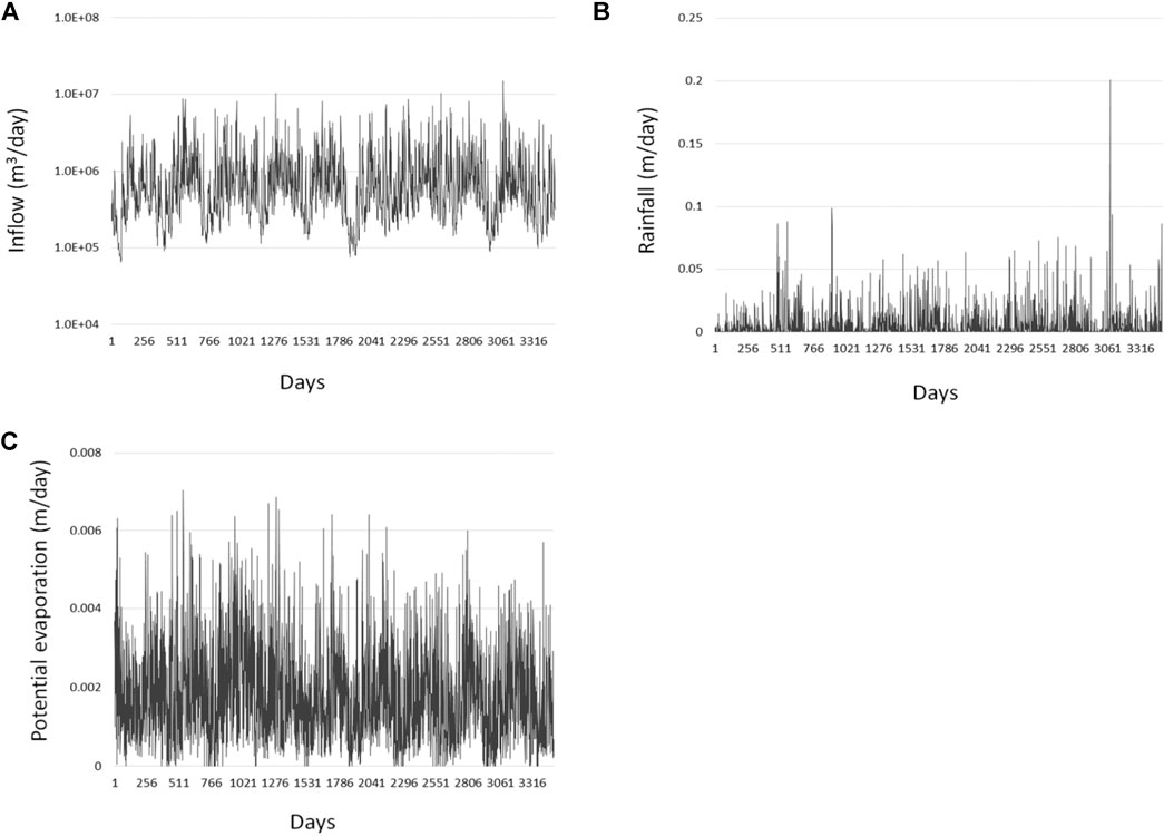
FIGURE 4. Time series of inputs for the synthetic model. (A) Upgradient inflows into reach 1, (B) rainfall; and (C) potential evaporation.

Figure 3A depicts 18 observation wells. In assessment of type 2 model shortcomings, steady state heads in nine of these wells (4, 5, 6, 10, 11, 12, 16, 17, 18) were selected for inclusion in the calibration dataset. Heads in these and other wells comprise model predictions. In analysis of type 3 model shortcomings, all 18 observation wells comprise the calibration dataset.

Model Parameters

Hydraulic property heterogeneity is represented using pilot points, the locations of which are shown in Figure 3A. Log-average values of 60 m/day and 0.01 are assumed for hydraulic conductivity and specific yield respectively. Spatial variability of both of these quantities is expressed by a log-exponential variogram with a range of 4.5 km; the sill of the log (to base 10) hydraulic conductivity variogram is 0.25 while that of the log specific yield variogram it is 0.0625. The high values of hydraulic conductivity and the low values of specific yield reflect conditions that prevail in many New Zealand catchments wherein groundwater flows through open framework gravels of extremely high permeability embedded in pervasive, clay-bound gravels of low specific yield.

Streambed and drain conductances along all of reaches 1 and 2 respectively are set to a uniform value of 1.0 m²/d. This is high enough to present minimal impediment to groundwater efflux into these streams. Nevertheless, these conductance parameters are included in the analyses described herein. The prior standard deviation attributed to the log of each of these conductances is 0.25.

Transient groundwater recharge is simulated using the LUMPREM lumped-parameter model. This is described by Watson et al. (2013) and Moeck et al. (2016). It is publicly available as Doherty (2020). LUMPREM simulates water balance within the plant root zone. It receives rainfall on a daily basis; water is lost as evapotranspiration, drainage recharge, macropore recharge and runoff. Nonlinear, user-parameterizable relationships govern the rates of evapotranspiration and below-root-zone drainage recharge as functions of soil moisture content. Time series of rainfall and potential evapotranspiration are shown in Figures 4B,C. The domain of the groundwater model is divided into four zones that are characterized by four different soil types, namely brown, pallic and two moderate soil types; see Figure 3B. A different instance of LUMPREM calculates recharge within each of these zones. Stochastic parameterization of these LUMPREM instances reflects the properties of these soil types, and a pasture vegetation type.

Model Timing

Time series of stream flow, rainfall and potential evapotranspiration for the 9 year simulation period which is the focus of the present study were extracted from much longer time series based on a much longer simulation time. This particular simulation time window was selected for the current study because of its following desirable features.

1. Borehole water levels show considerable variation over this time, with a range of more than 2 m at the upper extent of the model where this variation is greatest, this reflecting the transient nature of the simulated system.

2. Borehole water levels at the end of this time period are not too different from those at its beginning, no more than 0.01 m at the upper extent of the model.

The first requirement contributes to the integrity of the study documented herein, and conclusions drawn from it. The second underpins our use of average heads as steady state heads. In real-world practice, where the quality and quantity of borehole water level measurements can vary over a model domain, a modeller may adopt a different, and perhaps somewhat subjective, scheme for assignment of steady state heads to different wells. In our case, the use of averaging as a mechanism for representation or steady state conditions eliminates subjectivity, at the same time as it explores the relationship between “steady state” and “average”.

For the numerical experiments which comprise the present investigation, the model is run twice over its 9 year simulation period—once for calibration purposes and once for predictive purposes. To eliminate extraneous contributions to model-calculated quantities, the same set of starting conditions is employed for both of these runs. These starting conditions were calculated during the longer model run from which the 9 year simulation period was extracted. For the 9 year calibration run (i.e., the first of the model runs), conditions are as described above. During the 9 year prediction period, two pumping wells are introduced to the model domain. Their locations are depicted in Figure 3A. Each of these wells pumps at a uniform rate of 2,500 m³/day for 6 months of each year; these are summer months in which evaporation is high and rainfall is low. The first pumping period commences at the start of the simulation; subsequent pumping periods begin on the same day of each subsequent year. Joint yearly extraction from these two wells amounts to about 14% of long-term average recharge into the entire model domain.

Steady State Model Calibration

As stated above, steady state quantities are calculated as averages of respective transient quantities over the 9 year simulation period. In particular:

• Average LUMPREM-calculated recharges are supplied as steady state recharges in each of the four recharge zones.

• Average stream inflows are used as up-catchment flows into reach 1.

• The calibration dataset is comprised of average heads in 9 of the 18 observation wells (see Figure 3A above), average groundwater inflows into reach 1, and average groundwater inflows into reach 2.

• However, in analyzing type 3 model shortcomings, average heads in all 18 observation wells comprise the calibration dataset.

Predictions

Analyses described in the previous section are applied to the following four transient predictions:

• Time-averaged heads in the 18 observation wells depicted in Figure 3A.

• Time-averaged drawdowns in each of these wells. Drawdown is calculated as average head over the 9 year simulation time when pumps are not operating (i.e., the calibration period) minus average head over the 9 year prediction period when pumps are operating.

• Average depletion of groundwater inflow into each of reaches 1 and 2. Depletion of groundwater inflow is calculated as average groundwater inflow over the calibration period minus average groundwater inflow over the prediction period.

• Total time during the 9 year prediction period over which flow in each of reaches 1 and 2 is less than the Q95 threshold for each of these reaches. The Q95 threshold is the value of flow that is exceeded 95 percent of the time during the 9 year calibration period.

This suite of predictions is typical of those that are commonly employed to examine the effects of proposed pumping on the health of nearby rivers and streams.

Spatial heterogeneity of hydraulic conductivity affects the direction of groundwater flow in the south western part of the model domain. The disposition of areas of high and low hydraulic conductivity in any hydraulic property realization that is drawn from the prior parameter probability distribution determines how much groundwater leaves the system through each of reaches 1 and 2. The distribution of specific yield also influences flow into both of these reaches; higher, up-catchment groundwater levels induce greater amounts of reach 2 inflow. The presence of reach 2 therefore induces the direction of groundwater flow to change with season; furthermore, seasonal variation in its flow direction is realization-dependent. Hence, as well as introducing uncertainty to predictions of groundwater inflow into both of reaches 1 and 2, hydraulic property heterogeneity also introduces uncertainty to the notion of “steady state”.

The fourth of the above predictions is sensitive to the timing of the growth and decay of cones of groundwater depression that surround the two pumping wells. Parameters which govern this process have the capacity to be informed by transient calibration. Uncertainties associated with predicted durations of low stream flow are therefore expected to be higher when they are made by a model that has been calibrated under steady state conditions, than by a model that has been calibrated under transient conditions.

Results

Model Predictions

Time series of heads in a number of representative wells during the 9 year calibration period in which pumps are not operating, and during the 9 year prediction period during which pumps are operating, are provided in Figure 5. Time series of aquifer inflows into reaches 1 and 2 during the calibration and prediction periods are provided in Figure 6. The mean parameters used to calculate values of predictions of management interest are listed in the Supplementary Material Table S1. The calculated predictions are listed in the Supplementary Material Tables S2, S3 and S4.

FIGURE 5

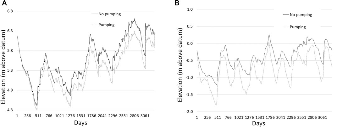
FIGURE 5. Time series of heads in two representative wells during the 9 year calibration period in which pumps are not operating, and during the 9 year prediction period during which pumps are operating. (A) Observation bore B2 located in the upper part of the groundwater model domain, and (B) observation bore B14 located in the lower part of the groundwater model domain.

FIGURE 6

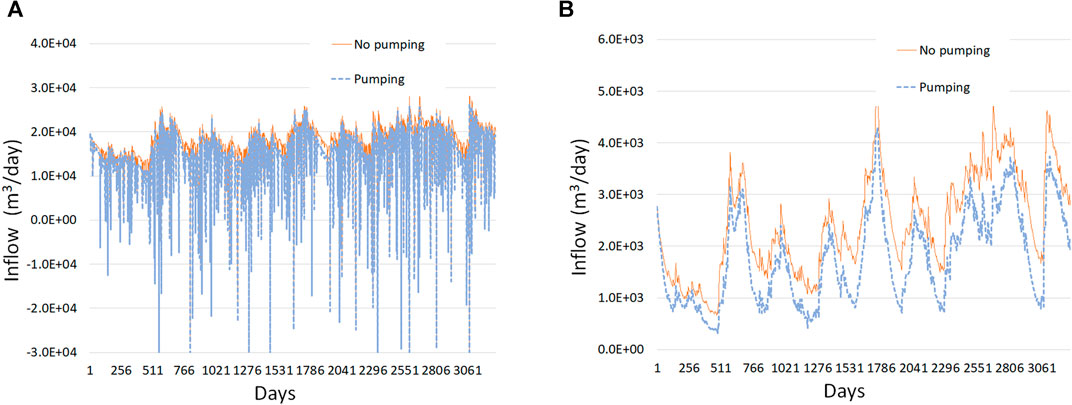
FIGURE 6. Time series of aquifer inflow into stream reaches 1 and 2 during the calibration and prediction periods for: (A) reach 1; and (B) reach 2.

Linear Analysis

Parameter Estimability

Before presenting the results of linear analysis as they pertain to the present study, we present a number of figures that depict other easily-achieved outcomes of linear analysis. They demonstrate the comparative capacity of steady state and transient calibration to reduce the posterior uncertainties of model parameters. It must be borne in mind, however, that the use of a model in decision-support depends on its ability to reduce the uncertainties of specific predictions, and not necessarily of parameters. Reducing the uncertainties of parameters to which predictions of management interest are not sensitive is therefore of secondary importance; this is further discussed below.

Figure 7A maps the relative posterior uncertainty of the log (to base 10) of hydraulic conductivity throughout the model domain attained through steady-state-only calibration. The relative posterior uncertainty, r, of a parameter is calculated as:

$r=\frac{{\mathit{\sigma }}_{\mathit{post}}}{{\mathit{\sigma }}_{\mathit{pre}}}(6)$

where σ_pre is the standard deviation of prior uncertainty of the parameter and σ_post is its standard deviation of its posterior uncertainty.

FIGURE 7

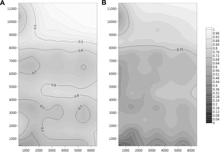
FIGURE 7. Maps of the relative posterior uncertainty of the log of hydraulic conductivity throughout the model domain attained through: (A) steady-state-only calibration, and (B) transient calibration.

Figure 7B maps this same statistic following transient calibration. These figures demonstrate the enhanced capacity of a transient dataset to inform hydraulic conductivity parameters, notwithstanding the fact that it must also inform other parameters.

Figure 8 maps the relative posterior uncertainty of the log of specific yield achieved through transient model calibration. This parameter type is not informed by steady-state-only model calibration. The ability of transient model calibration to reduce the uncertainty of this parameter type is readily apparent from this figure.

FIGURE 8

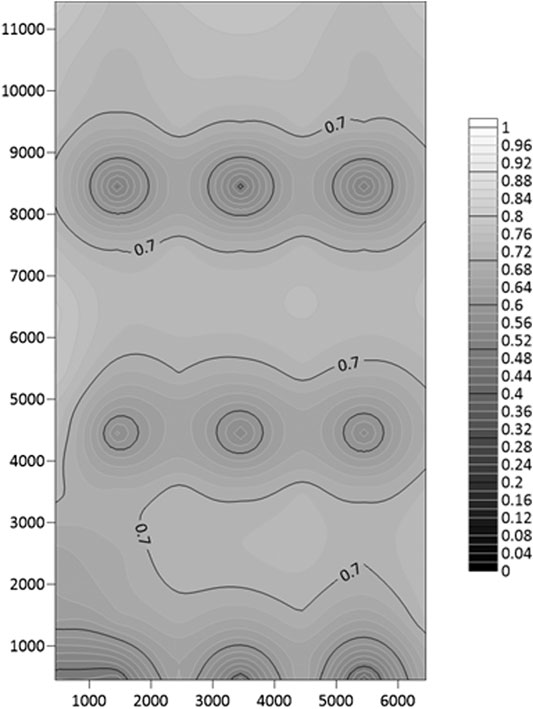
FIGURE 8. Map of the relative posterior uncertainty of the log of specific yield achieved through transient calibration.

Figure 9 charts relative posterior uncertainties of parameters belonging to the four soil-specific instances of the LUMPREM recharge model achieved through both steady state and transient calibration of the composite recharge/groundwater model. The back row of this figure shows relative posterior uncertainties achieved through steady-state-only calibration, whereas the front row shows relative posterior uncertainties achieved through transient calibration. Even though recharge is a transient phenomenon, steady-state-only calibration has a small capacity to reduce the uncertainties of LUMPREM parameters because time-averaged LUMPREM-calculated recharges are provided to the steady state version of the groundwater model.

FIGURE 9

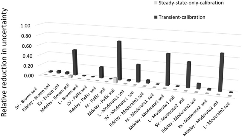
FIGURE 9. Relative reduction in LUMPREM parameter uncertainties achieved through history-matching to transient (back row) and steady state data (front row).

Analysis of Type 2 Shortcomings

We now consider the predictions which are the focus of the present study.

Figures 10A,B show the uncertainties associated with heads and drawdowns in all of the wells depicted in Figure 3A. Each of these figures has three rows. The back row provides standard deviations of prior prediction uncertainty. The middle row provides prediction standard deviations posterior to steady-state-only calibration. The front row provides prediction standard deviations posterior to transient calibration. These figures indicate that steady-state-only calibration considerably reduces the uncertainties of average head predictions, and that further uncertainty reductions accrued through transient calibration are small. The same does not apply to predictions of drawdown. These predictions benefit from the ability of transient history-matching to access extra information.

FIGURE 10

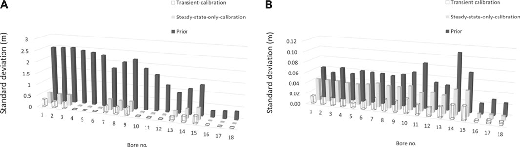
FIGURE 10. Uncertainties associated with predictions of pumping impacts on: (A) average groundwater levels in monitoring wells 1–18; and (B) average drawdowns in monitoring wells 1–18.

Figures 11A,B depict uncertainties associated with stream flow predictions in reaches 1 and 2. The same protocols are adopted for the three rows of each of these figures as are adopted for those of the previous figure. Figure 11A pertains to average stream flow depletion while Figure 11B pertains to flow duration below the Q95 level.

FIGURE 11

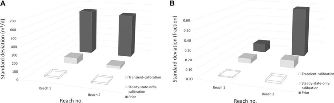
FIGURE 11. Uncertainties associated with predictions of: (A) the average stream depletion rate in reach 1 and reach 2; (B) the proportion of days below the low flow threshold (Q95) in reach 1 and reach 2.

It is apparent from Figure 11A that transient calibration adds little to the ability of steady state calibration to reduce uncertainties associated with predictions of average stream flow depletion in each of the reaches. This follows from the sensitivity of this prediction to local hydraulic conductivity (especially in the south west of the model domain), and from the ability of steady state calibration to inform this hydraulic property.

Factors that affect prolongation of low-flow conditions are more complex however (Figure 11B). The prior uncertainty of flow duration below the Q95 threshold is greater for reach 2 than for reach 1. This is because groundwater inflows are smaller into reach 2 than into reach 1, and because these inflows are sensitive to local aquifer properties. Steady-state-only calibration reduces the uncertainty of this prediction considerably because of its capacity to illuminate these local aquifer properties. For reach 1 however (for which groundwater inflows are much greater and are less affected by local aquifer properties), transient calibration is more effective, as it informs hydraulic properties that affect timing of drawdown propagation from the two pumping wells.

Nonlinear Analysis

In implementing the nonlinear methodology described in the previous section, a total of 200 parameter sets were drawn from the prior parameter probability distribution. As has already been discussed, for each of these realizations, a set of steady state observations was generated by running the transient model over the 9-year calibration period, and then averaging pertinent model outputs. A steady state model was calibrated against each of these sets of outputs. For each parameter realization, both pairs of model parameters (original and calibrated) were then used to make predictions which are the subject of this synthetic study.

Predictions made by all model pairs can be compared in a scatter plot. For a given parameter realization, a prediction made by the model which was calibrated under steady state conditions is plotted on the x axis. The prediction made using the original parameter realization is referred to the y axis.

We select two observation wells to exemplify the outcomes of this analysis, namely wells B2 and B14. These wells demonstrate worst and best performance of steady-state-only calibration in terms of its propensity to induce bias in these types of model prediction. Figures 12A,B pertain to average heads in these two wells over the prediction period in which pumps are operating, while Figures 13A,B pertain to average predicted drawdowns.

FIGURE 12

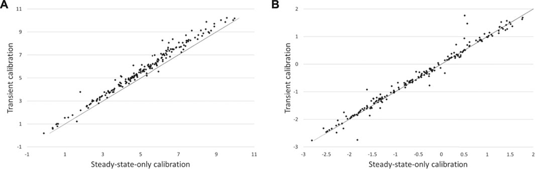
FIGURE 12. Nonlinear analysis of groundwater level predictions in: (A) upgradient bore B2; and (B) downgradient bore B14. Predictions made using the steady-state-calibrated parameter set are plotted on the x axis while those made using the original parameter set are plotted on the y axis.

FIGURE 13

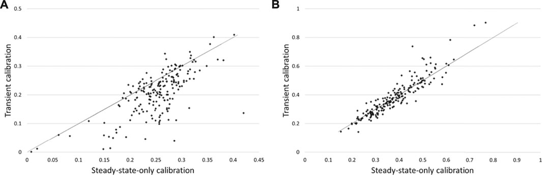
FIGURE 13. Nonlinear analysis of groundwater drawdown in: (A) upgradient bore B2; and (B) downgradient bore B14. Predictions made using the steady-state-calibrated parameter set are plotted on the x axis while those made using the original parameter set are plotted on the y axis.

The results for well B2 indicate a consistent bias for heads predicted by the steady-state-calibrated model, and an opposite bias for predicted drawdowns. In contrast, no such bias is apparent for well B14. Well B2 is situated in the upper part of the catchment, while B14 is situated closer to its outlet.

Under-prediction of B14 heads by the steady-state-calibrated model suggests a consistent overestimation of hydraulic conductivities in parts of the model domain. An examination of experimental results demonstrates that this is indeed the case. For some realizations, during very wet events the water table rises to the surface for a short period of time over parts of the model domain, this inducing saturated overland flow. Groundwater heads are thereby clipped. This introduces nonlinearity into the averaging process whereby average heads are derived from transient heads. With some averaged heads thereby biased low, local hydraulic conductivities inferred from these heads through steady state calibration are biased high.

Figures 14A,B show s vs s scatter plots for average groundwater inflow depletion into reaches 1 and 2. Predictions for reach 1 exhibit some degree of bias; there is tendency for the steady-state-calibrated model to over-predict pumping-induced flow depletion in this reach. We attribute this to the same phenomenon as that discussed above for B2 heads. Steady state calibration has a tendency to overestimate hydraulic conductivities in parts of the model domain, including those parts where extraction wells are situated. Higher hydraulic conductivities enable faster drawdown propagation to river reaches when these pumps are operating. This applies particularly to reach 1, as large parts of reach 2 are disconnected from the groundwater system during dry times when pumping occurs.

FIGURE 14

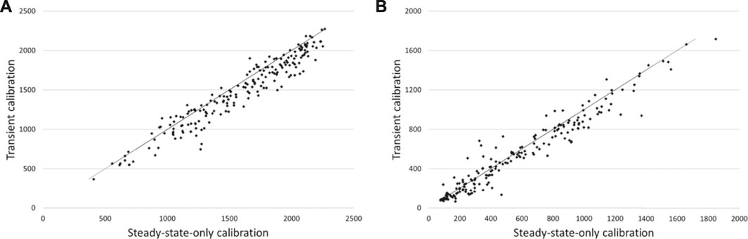
FIGURE 14. Nonlinear analysis of stream depletion predictions in reach 1 and reach 2: (A) Mean stream depletion rate in reach 1; (B) mean stream depletion rate in reach 2. Predictions made using the steady-state-calibrated parameter set are plotted on the x axis while those made using the original parameter set are plotted on the y axis.

Figures 15A,B provide s vs s scatter plots for the fraction of time over which flows in reaches 1 and 2 are less than their respective Q95 thresholds. Little steady-state-calibration-induced bias is apparent in this prediction for reach 1; however, there is a tendency for underestimation of this quantity in reach 2 by the steady-state-calibrated model.

FIGURE 15

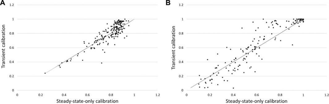
FIGURE 15. Nonlinear analysis of stream depletion predictions in reach 1 and reach 2. (A) Proportion of days below the low flow threshold in reach 1; (B) proportion of days below the low flow threshold in reach 2. Predictions made using the steady-state-calibrated parameter set are plotted on the x axis while those made using the original parameter set are plotted on the y axis.

Discussion

The results presented above suggest that steady-state-only model calibration can indeed reduce uncertainties associated with the predicted effects of pumping on nearby groundwater heads and inflows to streams. Furthermore, this reduction is significant. This reflects the high information content of steady state measurements with respect to conductance parameters such as hydraulic conductivity. Other studies (for example Gallagher and Doherty, 2007; Soltanian and Ritzi 2014) describe how hydraulic conductivity is often the major contributor to the uncertainties of many predictions of management interest. This follows from the large range of values that it may take, and its high degree of spatial variability.

However, where timing is important to a prediction, transient calibration can reap further uncertainty reduction benefits. Whether these benefits justify the construction and calibration of a transient model is a site-specific matter. The study reported herein demonstrates that this matter can be rapidly investigated by constructing a representative transient model, and then using that model for linear analysis. This is a far less onerous process than building a more detailed transient model, and then calibrating that model against actual field measurements. Linear analysis undertaken on the representative transient model can be used to explore whether the latter process is worth the effort.

Of greater concern is the propensity for steady-state-only calibration to induce bias in some decision-critical model predictions. The propensity for bias depends on the prediction, for some predictions are more susceptible to it than others. It also depends on the uncertainty associated with that prediction. If a prediction is highly uncertain, then errors introduced by bias may be small in comparison with this uncertainty. On the other hand, analyses such as those presented by White et al. (2014) suggest that the errors introduced by bias could be large for some predictions whose post-calibration uncertainties are apparently small.

In the present study, bias arises from the artificial nature of the steady state condition. It also arises from the manner in which steady state observations are computed from real observations. If steady state observations suffer bias, then inferences of hydraulic conductivity drawn from steady state calibration also suffer bias. This is demonstrated in the synthetic case discussed above where steady state heads are calculated by averaging transient heads. Occasional surface clipping of the latter during times of high rainfall introduces nonlinearities into the averaging process that bias calibrated hydraulic conductivities in parts of the model domain.

Removal of this particular source of bias would require that the calibration process eschew as close a fit with average heads as was achieved in the present study. This can be achieved in a number of ways. For example, the target objective function can be set to a higher value than that employed herein, lower weights can be assigned to time-averaged heads that are most likely to be affected by this process, or these heads can be removed from the calibration dataset altogether. More sophisticated accommodation of this source of bias may account for temporal correlation of head-averaging errors by designing a C(ε) matrix with appropriate off-diagonal elements. All of these options would induce higher uncertainties in some, if not all, management-salient predictions. This trade-off of increased uncertainty against reduced propensity for bias is not uncommon in data processing generally.

Steady state model calibration offers other opportunities for introduction of predictive bias. Whether this bias is any greater than that introduced through transient calibration is a matter of conjecture. In the present example we compute steady state recharge by averaging LUMPREM-calculated recharge over a 9 year period. At the same time, the calibration process was chosen to be representative of long term conditions, as it is reasonably lengthy and begins and ends with roughly the same amount of water stored underground. In real-world modelling practice, other estimates of steady state recharge may be employed. These are likely to have their own biases. For example they may lack spatial resolution, and/or the capacity to reflect different land uses and soil types; they may fail to account for local ponding during wet seasons wherein recharge is concentrated in certain areas. However calculation of transient recharge may suffer from similar problems, especially during periods of high rainfall (and therefore high recharge) where partitioning of water between runoff, interflow, ponding, macropore recharge and replenishment of the soil moisture store is notoriously difficult.

In the example discussed above, a model that undergoes steady-state-only calibration is used to make a transient prediction, i.e., the period of time over which stream flows are less than their Q95 levels. Under circumstances such as these, the parameters of the recharge model undergo very little adjustment during the regularized inversion process through which steady state model calibration is achieved. Their posterior uncertainties are therefore barely reduced from their prior uncertainties. Linear analysis demonstrates that if we can associate a range of recharge model parameter values with a particular soil and vegetation type (i.e., if we know the joint prior probability distribution of these parameters), then the uncertainties of some decision-critical model predictions may not suffer too much from this model-deployment strategy. However predictive uncertainty analysis becomes important under these circumstances. If a prediction of management interest is made using only a single set of recharge model parameter values that are central with respect to the joint prior parameter probability distribution, nonlinearity of recharge with respect to these parameters may engender considerable predictive bias. Fortunately, this is exposed and accommodated if the prediction is made using many parameter values that collectively sample the posterior parameter probability distribution, as is demonstrated in this study.

Conclusion

Environmental governance requires that responses be made on a regular basis to applications for increased groundwater extraction. A key adjudication criterion is the effect of the proposed pumping on nearby streams. Groundwater extraction has the capacity to reduce, or even eliminate, stream flows in dry seasons. Flow reduction can have a dramatic effect on stream water quality. This can have profoundly negative consequences for biota which inhabit streams.

Increased groundwater extraction can also impact existing groundwater users. It can lower the piezometric surface below present pump intake levels. In severe circumstances, it can make access to groundwater difficult during prolonged dry periods when demand for its use is greatest.

Calculations required for assessment of a licensing application are often based on modelling. However numerical modelling of natural systems is always compromised. Budgets are always lean; data are always scarce. A decision for or against a particular modelling strategy can never be conclusive. Nevertheless, model design and deployment decisions must be made. These decisions require metrics for success and failure. This paper presents generally-applicable metrics that can serve as reference points for adoption (or not) of a modelling strategy that involves steady-state-only calibration. It also demonstrates analysis methodologies through which adoption of this strategy can be judged against these metrics in a particular management context.

In real-world modelling practice, construction and calibration of a steady state model is not a particularly difficult undertaking. Software that implements highly parameterized inversion and data assimilation is readily available, and relatively easy to apply to steady state model calibration. A modeller can therefore readily extract information from a local steady state dataset. Management-critical predictions can then be made, and their uncertainties analysed. For some model predictions, these uncertainties will not be too much greater than if a more laborious process of construction and calibration of a transient model had been undertaken. Steady-state-only model calibration may therefore, in many cases, mark the point of diminishing return as far as decision-support modelling is concerned.

However, the present paper makes it clear that caution must be exercised. While the results documented herein suggest that transient history-matching does not reduce the uncertainties of some management-salient predictions too much below that which steady-state-only history-matching can achieve, these conclusions are location-specific and prediction-specific. In more general situations, the potential benefits of transient model calibration can be tested using the linear methods presented in this paper. The transient model that is used for this analysis need not be as complex as that which would actually be built and deployed for decision-support. Nor does it even need to be calibrated.

The potential for predictive bias that is incurred by the steady state assumption is more difficult to quantify. Strategies that reduce this potential are necessarily location-specific and prediction-specific. The extent to which they are a cause for concern is determined by the uncertainty of management-salient predictions. If these are large, the potential for error incurred by predictive bias may be small in comparison; it can therefore be neglected. Alternatively, if the potential for predictive bias is significant in comparison with the uncertainty of an important prediction, then it must be included in uncertainty intervals that are associated with this prediction. Rapid evaluation of the contribution of calibration-induced predictive bias to overall posterior predictive uncertainty in a range of modelling contexts is a matter that awaits further research.

Data Availability Statement

The original contribution presented in the study are included in the article/Supplementary Material, further inquiries can be directed to the corresponding author.

Author Contributions

CM undertook all numerical work. CM and JD jointly developed ideas expressed herein, and wrote the manuscript in partnership.

Funding

This work was funded, in part, through the “Smart Models for Aquifer Management” (SAM) research program Grant Number: C05X1508 funded by the New Zealand Ministry of Business, Innovation and Employment, and was also supported by GNS Science Groundwater Strategic Science Investment Fund (SSIF).

Conflict of Interest

JD was employed by Watermark Numerical Computing.

The remaining author declares that the research was conducted in the absence of any commercial or financial relationships that could be construed as a potential conflict of interest.

Publisher’s Note

All claims expressed in this article are solely those of the authors and do not necessarily represent those of their affiliated organizations or those of the publisher, the editors, and the reviewers. Any product that may be evaluated in this article, or claim that may be made by its manufacturer, is not guaranteed or endorsed by the publisher.

Supplementary Material

The Supplementary Material for this article can be found online at: https://www.frontiersin.org/articles/10.3389/feart.2021.692671/full#supplementary-material

References

Cooley, R. L., and Christensen, S. (2006). Bias and Uncertainty in Regression-Calibrated Models of Groundwater Flow in Heterogeneous media. Adv. Water Resour. 29 (5), 639–656. doi:10.1016/j.advwatres.2005.07.012

CrossRef Full Text | Google Scholar

Crosbie, R. S., Peeters, L. J. M., Herron, N., McVicar, T. R., and Herr, A. (2018). Estimating Groundwater Recharge and its Associated Uncertainty: Use of Regression Kriging and the Chloride Mass Balance Method. J. Hydrol. 561, 1063–1080. doi:10.1016/j.jhydrol.2017.08.003

CrossRef Full Text | Google Scholar

Doherty, J., and Christensen, S. (2011). Use of Paired Simple and Complex Models to Reduce Predictive Bias and Quantify Uncertainty. Water Resour. Res. 47, W12534. doi:10.1029/2011WR010763

CrossRef Full Text | Google Scholar

Doherty, J., and Moore, C. (2019). Decision Support Modeling: Data Assimilation, Uncertainty Quantification, and Strategic Abstraction. Groundwater 58, 327–337. doi:10.1111/gwat.12969

PubMed Abstract | CrossRef Full Text | Google Scholar

Doherty, J., and Simmons, C. T. (2013). Groundwater Modelling in Decision Support: Reflections on a Unified Conceptual Framework. Hydrogeol J. 21, 1531–1537. doi:10.1007/s10040-013-1027-7

CrossRef Full Text | Google Scholar

Doherty, J. (2003). Ground Water Model Calibration Using Pilot Points and Regularization. Ground Water 41 (2), 170–177. doi:10.1111/j.1745-6584.2003.tb02580.x

PubMed Abstract | CrossRef Full Text | Google Scholar

Doherty, J., (2015). Calibration and Uncertainty Analysis for Complex Environmental Models. Brisbane, Australia: Watermark Numerical Computing. 227pp. ISBN: 978-0-9943786-0-6. Downloadable from www.pesthomepage.org

Doherty, J. (2020). PEST: Model-independent Parameter Estimation. Brisbane, Australia: Watermark Numerical Computing. Downloadable from www.pesthomepage.org

Google Scholar

Farthing, M. W., and Ogden, F. L. (2017). Numerical Solution of Richards' Equation: A Review of Advances and Challenges. Soil Sci. Soc. Am. J. 81, 1257–1269. doi:10.2136/sssaj2017.02.0058

CrossRef Full Text | Google Scholar

Freeze, R. A., Massmann, J., Smith, L., Sperling, T., and James, B. (1990). Hydrogeological Decision Analysis: 1. A Framework. Groundwater 28 (5), 738–766. doi:10.1111/j.1745-6584.1990.tb01989.x

CrossRef Full Text | Google Scholar

Gallagher, M., and Doherty, J. (2007). Predictive Error Analysis for a Water Resource Management Model. J. Hydrol. 34 (3-4), 513–533. doi:10.1016/j.jhydrol.2006.10.037

CrossRef Full Text | Google Scholar

Healy, R. W., and Scanlon, B. R. (2010). “Physical Methods: Unsaturated Zone,” in Estimating Groundwater Recharge (Cambridge: Cambridge University Press), 97–116. doi:10.1017/CBO9780511780745.006

CrossRef Full Text | Google Scholar

Hemmings, B., Knowling, M. J., and Moore, C. R. (2020). Early Uncertainty Quantification for an Improved Decision Support Modeling Workflow: A Streamflow Reliability and Water Quality Example. Front. Earth Sci. 8, 502. doi:10.3389/feart.2020.565613

CrossRef Full Text | Google Scholar

Hocking, M., and Kelly, B. F. J. (2016). Groundwater Recharge and Time Lag Measurement through Vertosols Using Impulse Response Functions. J. Hydrol. 535, 22–35. doi:10.1016/j.jhydrol.2016.01.042

CrossRef Full Text | Google Scholar

Kennedy, M. C., and O'Hagan, A. (2001). Bayesian Calibration of Computer Models. J. R. Stat. Soc. Ser. B (Stat Methodol). 63 (3), 425–464. doi:10.1111/1467-9868.00294

CrossRef Full Text | Google Scholar

Knowling, M. J., White, J. T., McDonald, G. W., Kim, J.-H., Moore, C. R., and Hemmings, B. (2020a). Disentangling Environmental and Economic Contributions to Hydro-Economic Model Output Uncertainty: An Example in the Context of Land-Use Change Impact Assessment. Environ. Model. Softw. 127, 104653. Available at: https://www.sciencedirect.com/science/article/pii/S1364815219305031?via%3Dihub. doi:10.1016/j.envsoft.2020.104653

CrossRef Full Text | Google Scholar

Knowling, M. J., White, J. T., Moore, C. R., Rakowski, P., and Hayley, K. (2020b). On the Assimilation of Environmental Tracer Observations for Model-Based Decision Support. Hydrol. Earth Syst. Sci. 24, 1677–1689. doi:10.5194/hess-24-1677-2020

CrossRef Full Text | Google Scholar

Moeck, C., Brunner, P., and Hunkeler, D. (2016). The Influence of Model Structure on Groundwater Recharge Rates in Climate-Change Impact Studies. Hydrogeol J. 24 (5), 1171–1184. doi:10.1007/s10040-016-1367-1

CrossRef Full Text | Google Scholar

Nicol, C., and Doherty, J. (2021). Exploring Model Defects Using Linear Analysis: A GMDSI Worked Example Report. South Australia: National Centre for Groundwater Research and Training, Flinders University. ISBN: 978-1-925562-52-1. DOI as a weblink. doi:10.25957/ew1j-9g7510.25957/ew1j-9g75

CrossRef Full Text

Niswonger, R. G., Panday, S., and Ibaraki, M. (2011). MODFLOW-NWT, A Newton Formulation for MODFLOW-2005: U.S. Geol. Surv. Tech. Methods 6-A37, 44.

Google Scholar

Oliver, D. S., and Alfonzo, M. (2018). Calibration of Imperfect Models to Biased Observations. Comput. Geosci. 22, 145–161. doi:10.1007/s10596-017-9678-4

CrossRef Full Text | Google Scholar

Schilling, O. S., Doherty, J., Kinzelbach, W., Wang, H., Yang, P. N., and Brunner, P. (2014). Using Tree Ring Data as a Proxy for Transpiration to Reduce Predictive Uncertainty of a Model Simulating Groundwater-Surface Water-Vegetation Interactions. J. Hydrol. 519, 2258–2271. doi:10.1016/j.jhydrol.2014.08.063

CrossRef Full Text | Google Scholar

Shaw, R. J., and Thorburn, P. J. (1985). Prediction of Leaching Fraction from Soil Properties, Irrigation Water and Rainfall. Irrig Sci. 6, 73–83. doi:10.1007/bf00251556

CrossRef Full Text | Google Scholar

Soltanian, M. R., and Ritzi, R. W. (2014). A New Method for Analysis of Variance of the Hydraulic and Reactive Attributes of Aquifers as Linked to Hierarchical and Multiscaled Sedimentary Architecture. Water Resour. Res. 50, 9766–9776. doi:10.1002/2014WR015468

CrossRef Full Text | Google Scholar

Watson, T. A., Doherty, J. E., and Christensen, S. (2013). Parameter and Predictive Outcomes of Model Simplification. Water Resour. Res. 49 (7), 3952–3977. doi:10.1002/wrcr.20145

CrossRef Full Text | Google Scholar

White, J. T., Doherty, J. E., and Hughes, J. D. (2014). Quantifying the Predictive Consequences of Model Error with Linear Subspace Analysis. Water Resour. Res. 50 (2), 1152–1173. doi:10.1002/2013WR014767

CrossRef Full Text | Google Scholar

White, J. T., Fienen, M. N., and Doherty, J. E. (2016). A python Framework for Environmental Model Uncertainty Analysis. Environ. Model. Softw. 85, 217–228. doi:10.1016/j.envsoft.2016.08.017

CrossRef Full Text | Google Scholar

White, J. T., Knowling, M. J., and Moore, C. R. (2019). Consequences of Groundwater‐Model Vertical Discretization in Risk‐Based Decision‐Making. Groundwater 58, 695–709. doi:10.1111/gwat.12957

PubMed Abstract | CrossRef Full Text | Google Scholar

White, J. T., Knowling, M. J., Fienen, M. N., Feinstein, D. T., McDonald, G. W., and Moore, C. R. (2020). A Non-intrusive Approach for Efficient Stochastic Emulation and Optimization of Model-Based Nitrate-Loading Management Decision Support. Environ. Model. Softw. 126, 104657. Available at: https://www.sciencedirect.com/science/article/pii/S1364815219309934?via%3Dihub. doi:10.1016/j.envsoft.2020.104657

CrossRef Full Text | Google Scholar

Wood, W. W. (1999). Use and Misuse of the Chloride-Mass Balance Method in Estimating Ground Water Recharge. Ground Water 37, 2–3. doi:10.1111/j.1745-6584.1999.tb00949.x

CrossRef Full Text | Google Scholar