Reverse Time Migration Based on the Pseudo-Space-Domain First-Order Velocity-Stress Acoustic Wave Equation

Reverse time migration (RTM) is an ideal seismic imaging method for complex structures. However, in conventional RTM based on rectangular mesh discretization, the medium interfaces are usually distorted. Besides, reflected waves generated by the two-way wave equation can cause artifacts during imaging. To overcome these problems, a high-order finite-difference (FD) scheme and stability condition for the pseudo-space-domain first-order velocity-stress acoustic wave equation were derived, and based on the staggered-grid FD scheme, the RTM of the pseudo-space-domain acoustic wave equation was implemented. Model experiments showed that the proposed RTM of the pseudo-space-domain acoustic wave equation could systematically avoid the interface distortion problem when the velocity interfaces were considered to compute the pseudo-space-domain intervals. Moreover, this method could effectively suppress the false scattering of dipping interfaces and reflections during wavefield extrapolation, thereby reducing migration artifacts on the profile and significantly improving the quality of migration imaging.

Introduction

Based on the theory of the two-way wave equation, the reverse time migration (RTM) algorithm was conceived in the early 1980s (McMechan, 1983; Whitmore, 1983). Since the wave equation does not need to be decomposed, there is no strata dip angle limitation caused by the wave equation approximation. The RTM is recognized as an ideal imaging method for complex structures and has been a popular topic in the field of geophysics (Moradpouri et al., 2017; Li et al., 2018; Zhou et al., 2018; Li et al., 2020). Chang and McMechan (1987) generalized the two-dimensional RTM to the elastic wavefield and then extended it to three dimensions (Chang and McMechan, 1990, 1994). Zhang and Ning (2002) proposed multi-wave and multi-component RTM based on the eikonal equation. Sun and McMechan (2001) implemented elastic wave RTM based on the separation of P- and S-waves. Yan (2012) studied the viscoelastic tilted transversely isotropic medium wave equation RTM algorithm based on rotating staggered grids. Liu et al. (2013) achieved RTM of elastic waves in porous media based on Biot’s theory. Song et al. (2015) proposed the RTM of divided-order multiples to solve the problem of imaging difficulty in the regions of low illumination based on primaries. In terms of computational efficiency and storage consumption, Liu et al. (2010) applied the graphics processing unit (GPU) for algorithmic acceleration, which greatly improved the computational efficiency of RTM. Clapp (2009) and Wang et al. (2012) used the random boundary and absorbing boundary storage strategies to reduce the consumption of storage capacity. Shi et al. (2015) analyzed the effect of random boundaries and an absorbing boundary in RTM and summarized the calculation cost and storage requirement for different boundaries and storage strategies.

After a few decades of development, the RTM technology has become increasingly mature, but it still suffers from the following problems: First, the RTM is usually achieved by using the finite-difference (FD) method with regular rectangular grids. When the underground interface model is meshed by grids, dipping interfaces and undulating surfaces only can be replaced by staircase curves, which may result in false scattering and interfacial distortion during RTM. In this respect, some scholars used variable space grids (Zhu and Wei, 2005, 2007; Huang and Dong, 2009), in which fine grids were adopted at regions with severe variation of medium parameters. However, this method still doesn’t eliminate the limitations of rectangular grids, and it increases computational cost. Chu and Wang (2005) proposed an FD simulation method based on an irregular triangular mesh used in the finite-element method. Compared with the traditional rectangular mesh FD scheme, this method can describe undulating interfaces better, but the computational complexity increased. Besides, now there are many studies on RTM from rugged topography using curvilinear meshing or unstructured triangular meshing to get rid of the staircase approximation (Lan et al., 2014; Shragge, 2014; Liu et al., 2016; Qu et al., 2019; Liu and Zhang, 2020). Second, in the conventional RTM wavefield extrapolation based on the two-way wave equation, it produces a large number of reflection waves (back-propagating waves) at the interfaces. On the migration profile, it forms strong low-frequency noises and artifacts generated by wavepath cross-correlation with forward- and back-propagating waves, which result in low-profile imaging quality (Du et al., 2013). To reduce the influence of reflection waves, Baysal et al. (1984) deduced that the non-reflection acoustic equation can suppress the reflection waves well in the case of small incident angle under the assumption of constant impedance of the underlying medium. On the basis of the non-reflection acoustic equation proposed by Baysal, Song (2005) realized a recursive method to calculate the non-reflection scalar wave equation by introducing a wave impedance function. Willacy and Kryvohuz (2019) tried to image steep boundaries between a salt body and surrounding sediments based on the RTM using transmitted waves. He et al. (2008) developed RTM of arbitrarily wide-angle wave equations, but the imaging effect of this method is poor in shallow regions. Yoon and Marfurt (2006) introduced Poynting vector imaging conditions into RTM to realize cross-correlation of different direction wavefields, but it has a big numerical error in the regions of complex tectonics. Liu et al. (2011) proposed an imaging condition of RTM based on wavefield decomposition that separated up-going and down-going waves by using the F-K transform; however, the method of separating wavefields required a large amount of extra calculation and storage.

The effective solution of above two problems is of great significance to improve the imaging quality of RTM. Wang et al. (2005) deduced a pseudo-space-domain scalar acoustic equation by transforming the traditional wave equation from the time-space domain to time-traveltime domain (or “traveltime domain”). This scheme not only overcomes the problem of seismic velocity interface distortion but also effectively suppresses false scattering and reflections. However, based on the second-order partial differential acoustic wave equation, Wang et al. (2005) had realized a second-order FD solution in pseudo-space domain using regular grid, which cannot meet the needs of calculation accuracy. Based on the detailed discussion of the principle of the pseudo-space-domain wave equation, this thesis derives the high-order staggered-grid FD scheme and stability condition for the pseudo-space-domain first-order velocity-stress wave equation and achieves high-precision RTM with them.

Pseudo-Space-Domain First-Order Velocity-Stress Acoustic Wave Equation

At present, the most of FD wavefield extrapolations of the acoustic wave are based on the first-order velocity-stress acoustic wave equation. It can be written as follows:

$\{\begin{array}{l}\rho \frac{\partial {\tilde{v}}_x}{\partial t}=-\frac{\partial \tilde{P}}{\partial x},\\ \rho \frac{\partial {\tilde{v}}_z}{\partial t}=-\frac{\partial \tilde{P}}{\partial z},\\ \frac{\partial \tilde{P}}{\partial t}=-\rho c_p^2\left(\frac{\partial {\tilde{v}}_x}{\partial x}+\frac{\partial {\tilde{v}}_z}{\partial z}\right)+s\left(t\right),\end{array}(1)$

where x and z represent the horizontal and vertical coordinates of the space domain, respectively, $c_p$ is the primary velocity at point $\left(x,z\right)$, $\rho$ is the density at point $\left(x,z\right)$, $\tilde{P}$ represents the pressure, ${\tilde{v}}_x$ and ${\tilde{v}}_z$ represent the velocity components in the x and z directions, respectively, $s\left(t\right)$ is the source function, with $t$ being time. To obtain the numerical solution of Eq. 1, we usually use differences instead of differentials to approximate derivatives based on the staggered-grid technique (Vireux, 1984).

The conventional FD method, which is applied to the acoustic equation, is based on rectangular grid. When the subsurface interface model is meshed, the dipping interface can only be described by using a staircase curve. It can cause false scattering in the process of wavefield extrapolation and interface distortion at the migration profile. At the same time, the two-way wave equation can generate reflected waves at the interfaces between different velocity layers. Furthermore, strong low-frequency noises and artifacts are formed on the migration profile, which lead to low profile imaging quality.

To solve above problems, a pseudo-space-domain first-order velocity-stress acoustic wave equation is proposed in this article. In RTM of acoustic wave equation, imaging about the pressure $\tilde{P}$ is usually used. Therefore, under the condition that the $\tilde{P}$ is not affected, assuming$v_x=c_p{\tilde{v}}_x$, $v_z=c_p{\tilde{v}}_z$, $P=\tilde{P}$, Eq. 1 can be transformed into

$\{\begin{array}{l}\frac{\partial v_x}{\partial t}=-\frac{c_p}{\rho }\frac{\partial P}{\partial x},\\ \frac{\partial v_z}{\partial t}=-\frac{c_p}{\rho }\frac{\partial P}{\partial z},\\ \frac{\partial P}{\partial t}=-\rho c_p\left(\frac{\partial v_x}{\partial x}+\frac{\partial v_z}{\partial z}\right)+s\left(t\right).\end{array}(2)$

After discretizing the continuous model into a grid model, we set the spatial unit grid length as $\Delta \xi$ (where $\xi$ can represent $x$ or $z$) and that the traveltime between a grid length $\Delta \xi$ as $\Delta {\tau }_{\xi }$. Then, the space grid $\Delta \xi$ and traveltime $\Delta {\tau }_{\xi }$ satisfy the relationship $\Delta \xi =c_p\Delta {\tau }_{\xi }$, where $c_p$ is the acoustic wave velocity in the grid point. The derivative of the pressure and velocity components with respect to space can be rewritten as:

$\{\begin{array}{l}\frac{\partial P}{\partial {\tau }_{\xi }}=c_p\frac{\partial P}{\partial \xi },\\ \frac{\partial v_x}{\partial {\tau }_{\xi }}=c_p\frac{\partial v_x}{\partial \xi },\\ \frac{\partial v_z}{\partial {\tau }_{\xi }}=c_p\frac{\partial v_z}{\partial \xi }.\end{array}(3)$

Then, substituting Eq. 3 into Eq. 1 yields Eq. 4, which is the pseudo-space-domain first-order velocity-stress acoustic wave equation.

$\{\begin{array}{l}\frac{\partial v_x}{\partial t}=-\frac{1}{\rho }\frac{\partial P}{\partial {\tau }_x},\\ \frac{\partial v_z}{\partial t}=-\frac{1}{\rho }\frac{\partial P}{\partial {\tau }_z},\\ \frac{\partial P}{\partial t}=-\rho \left(\frac{\partial v_x}{\partial {\tau }_x}+\frac{\partial v_z}{\partial {\tau }_z}\right)+s\left(t\right).\end{array}(4)$

Numerical Simulation of the Pseudo-Space-Domain First-Order Velocity-Stress Acoustic Equation

Sampling Interval Calculation in the Pseudo-Space-Domain

Usually, to solve Eq. 4 by the FD method, first we should discretize the continuous model into a grid model and then compute the “traveltime” $\Delta {\tau }_{\xi }$ along with the grid point interval $\Delta \xi$. For simplicity, $\Delta {\tau }_{\xi }$ is called the “pseudo-space-domain interval”.

In the two-dimensional case, there are four pseudo-space-domain intervals at a point $P\left(i,j\right)$, where $i$ and $j$represent grid coordinates in the $x$ and $z$ directions, respectively. In the following discussion, a pseudo-space-domain interval is denoted as $\Delta {\tau }_l^{\pm }\left(i,j\right)$, where $l$ represents $i$ or $j$, “−” and “+” represent the side of the smaller coordinate grid number and the side of the larger coordinate grid number, respectively. As shown in Figure 1, $\Delta {\tau }_i^{-}\left(i,j\right)$ represents the pseudo-space-domain interval between points $P\left(i-1,j\right)$ and $P\left(i,j\right)$, $\Delta {\tau }_j^{-}\left(i,j\right)$ represents the pseudo-space-domain interval between points $P\left(i,j-1\right)$ and $P(i,j)$, $\Delta {\tau }_i^{+}\left(i,j\right)$ represents the pseudo-space-domain interval between points $P\left(i+1,j\right)$ and $P\left(i,j\right)$, and $\Delta {\tau }_j^{+}\left(i,j\right)$ represents the pseudo-space-domain interval between points $P\left(i,j+1\right)$ and $P\left(i,j\right)$.

FIGURE 1

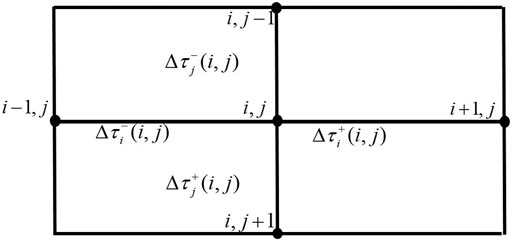
FIGURE 1. Four pseudo-space-domain intervals at the point $P\left(i,j\right)$.

Obviously, there are no velocity parameter items in Eq. 4. When the wave equation is transformed into pseudo-space domain, the original discrete space grid point velocity information is assigned to a grid line. At the same time, additional velocity information of the interfaces intersected on grid lines can be provided for computing the pseudo-space-domain intervals. Figure 2 shows a partial schematic illustration of a mesh model after the regular meshing of a velocity interface model including a dipping interface (as shown by the black solid line in Figure 2). The primary velocities at the upper and lower sides of the interface are 3,000 and 3,500 m/s, respectively, and the grid interval is 10 m. It can be seen that, after meshing the velocity interface model according to a regular rectangular grid, the dipping interface is distorted to an obvious staircase fold line. However, in the pseudo-space-domain, the “propagation time” on both sides of the velocity interface is calculated according to its actual velocity and propagation distance, and the time sampling interval corresponding to the grid line is the sum of different “time of propagation” segments. Points P and Q in Figure 2 are two adjacent spatial grid points after the velocity model is divided according to a rectangular grid, and the velocity interface as shown by the black solid line intersects segment PQ at point B. In this case, the pseudo-space-domain interval between P and Q may be calculated as $\Delta \tau =\Delta {\tau }_{PB}+\Delta {\tau }_{BQ}$, where $\Delta {\tau }_{PB}$ is the traveltime along with segment PB, and$\Delta {\tau }_{BQ}$ is the traveltime along segment BQ.

FIGURE 2

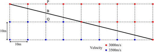
FIGURE 2. Partial schematic illustration of a mesh model after the regular meshing of a velocity interface model including a dipping interface.

Theoretically, there is no longer a distortion of the velocity interface in the pseudo-space-domain, and even the mutation of the model parameters between adjacent grid points are weakened, so it is expected that false scattering and interface reflection in the migration calculation can be reduced.

A 2Nth-Order-Accuracy Staggered-Grid FD Scheme of the Pseudo-Space-Domain First-Order Velocity-Stress Acoustic Wave Equation

In the implementation of FD numerical simulations based on the pseudo-space-domain acoustic wave equation, as well as to improve the accuracy of the simulation and suppress the impact of numerical dispersion, we need to improve the accuracy of the differences. Therefore, in this study, we deduce the 2Nth-order-accuracy staggered-grid FD expression for the acoustic wave equation in the pseudo-space-domain.

In the two-dimensional case, the coordinates are denoted as $\left(i,j\right)$ in the space-domain model discretized by sampling interval $\left(\Delta x,\Delta z\right)$. The corresponding coordinates of the pseudo-space-domain are $\left({\tau }_i,{\tau }_j\right)$. We take $\frac{\partial P}{\partial {\tau }_x}$ and $\frac{\partial v_x}{\partial {\tau }_x}$ as examples to give the propagation time interval calculation formula in pseudo-space-domain.

When calculating $\frac{\partial P}{\partial {\tau }_x}$ at ${\tau }_x={\tau }_{i+1/2}$, $P$ is located at point $\left({\tau }_{i+m},{\tau }_j\right)$ and $\left({\tau }_{i-\left(m-1\right)},{\tau }_j\right)\left(m=\mathrm{1,2,3},\dots \right)$. In the ${\tau }_x$ direction, the pseudo-space-domain propagation time intervals centered on$\left({\tau }_{i+1/2},{\tau }_j\right)$ are shown as follows:

$\Delta {\tau }_{i+1/2}^{+m}=\{\begin{array}{cc}0.5\Delta {\tau }_i^{+}\left(i,j\right)& \left(m=1\right),\\ 0.5\Delta {\tau }_i^{+}\left(i,j\right)+{\displaystyle \sum _{k=1}^{m-1}\Delta {\tau }_i^{+}\left(i+k,j\right)}& \left(m>1\right),\end{array}(5)$

where $\Delta {\tau }_i^{+}\left(i+k,j\right)$ represents the pseudo-space-domain interval between points $\left(i+k,j\right)$ and$\left(i+1+k,j\right)$, $\Delta {\tau }_{i+1/2}^{+m}$ represents the propagation time interval between $\left({\tau }_{i+1/2},{\tau }_j\right)$ and the grid point $\left({\tau }_{i+m},{\tau }_j\right)$ where $P$ is located.

$\Delta {\tau }_{i+1/2}^{-\left(m-1\right)}=\{\begin{array}{cc}0.5\Delta {\tau }_i^{+}\left(i,j\right)& \left(m=1\right),\\ 0.5\Delta {\tau }_i^{+}\left(i,j\right)+{\displaystyle \sum _{k=0}^{m-2}\Delta {\tau }_i^{-}\left(i-k,j\right)}& \left(m>1\right),\end{array}(6)$

where $\Delta {\tau }_i^{-}\left(i-k,j\right)$ represents the pseudo-space-domain interval between points $\left(i-1-k,j\right)$ and $\left(i-k,j\right)$, $\Delta {\tau }_{i+1/2}^{-\left(m-1\right)}$ represents the propagation time interval between $\left({\tau }_{i+1/2},{\tau }_j\right)$ and the grid point $\left({\tau }_{i-\left(m-1\right)},{\tau }_j\right)$ where $P$ is located. It notes that here and hereinafter $\left({\tau }_{i+1/2},{\tau }_j\right)$ indicates the center point of the propagation time between $\left(i,j\right)$ and $\left(i+1,j\right)$.

When calculating $\frac{\partial v_x}{\partial {\tau }_x}$ at ${\tau }_x={\tau }_i$, velocity $v_x$ is located at point $\left({\tau }_{i+\left(m-1/2\right)},{\tau }_j\right)$ and $\left({\tau }_{i-\left(m-1/2\right)},{\tau }_j\right)\left(m=\mathrm{1,2,3},\dots \right)$. In the ${\tau }_x$ direction, the pseudo-space-domain propagation time intervals centered on $\left({\tau }_i,{\tau }_j\right)$ are shown as follows.

$\Delta {\tau }_i^{+\left(m-1/2\right)}=\{\begin{array}{cc}0.5\Delta {\tau }_i^{+}\left(i,j\right)& \left(m=1\right),\\ 0.5\Delta {\tau }_i^{+}\left(i+m-1,j\right)+{\displaystyle \sum _{k=0}^{m-2}\Delta {\tau }_i^{+}\left(i+k,j\right)}& \left(m>1\right),\end{array}(7)$

where $\Delta {\tau }_i^{+}\left(i+k,j\right)$ represents the pseudo-space-domain interval between points $(i+k,j)$ and $(i+1+k,j)$, and $\Delta {\tau }_i^{+(m-1/2)}$ represents the propagation time interval between $({\tau }_i,{\tau }_j)$ and the grid point $({\tau }_{i+(m-1/2)},{\tau }_j)$ where $v_x$ is located.

$\Delta {\tau }_i^{-\left(m-1/2\right)}=\{\begin{array}{cc}0.5\Delta {\tau }_i^{-}\left(i,j\right)& \left(m=1\right),\\ 0.5\Delta {\tau }_i^{-}\left(i-m+1,j\right)+{\displaystyle \sum _{k=0}^{m-2}\Delta {\tau }_i^{-}\left(i-k,j\right)}& \left(m>1\right),\end{array}(8)$

where $\Delta {\tau }_i^{-}\left(i-k,j\right)$ represents the pseudo-space-domain interval between points $\left(i-1-k,j\right)$ and $\left(i-k,j\right)$, and $\Delta {\tau }_i^{-\left(m-1/2\right)}$ represents the propagation time interval between $\left({\tau }_i,{\tau }_j\right)$ and the grid point $\left({\tau }_{i-\left(m-1/2\right)},{\tau }_j\right)$ where $v_x$ is located. Similarly, the pseudo-space-domain propagation time interval of $P$ and $v_z$ in the direction ${\tau }_z$ can be calculated separately in a similar manner as described above.

Using the propagation time interval shown in Eqs 5, 6, the 2Nth-order-accuracy expansion of the first-order derivative of the $P$ with respect to the variable ${\tau }_x$ can be obtained. The $P$ in the pseudo-space-domain is assumed to have a 2Nth-order derivative. For different $P_{{\tau }_x}$values, satisfying ${\tau }_x={\tau }_{i+1/2}+\Delta {\tau }_{i+1/2}^{+m}$ and ${\tau }_x={\tau }_{i+1/2}-\Delta {\tau }_{i+1/2}^{-\left(m-1\right)}$ corresponding to ${\tau }_x={\tau }_{i+m}$ and ${\tau }_x={\tau }_{i-\left(m-1\right)}$ ($m$=$\mathrm{1,2},\dots ,N-1,N$), respectively, the 2Nth-order Taylor series expansions at ${\tau }_x={\tau }_{i+1/2}$ are

$P_{{\tau }_{i+1/2}+\Delta {\tau }_{i+1/2}^{+m}}=P_{{\tau }_{i+1/2}}+{\displaystyle \sum _{n=1}^{2N-1}\frac{{\left(+\Delta {\tau }_{i+1/2}^{+m}\right)}^n}{n!}{P}_{{\tau }_{i+1/2}}^{\left(n\right)}}+O\left({\left(+\Delta {\tau }_{i+1/2}^{+m}\right)}^{2N}\right),(9)$

$P_{{\tau }_{i+1/2}-\Delta {\tau }_{i+1/2}^{-\left(m-1\right)}}=P_{{\tau }_{i+1/2}}+{\displaystyle \sum _{n=1}^{2N-1}\frac{{\left(-\Delta {\tau }_{i+1/2}^{-\left(m-1\right)}\right)}^n}{n!}{P}_{{\tau }_{i+1/2}}^{\left(n\right)}}+O\left({\left(-\Delta {\tau }_{i+1/2}^{-\left(m-1\right)}\right)}^{2N}\right),(10)$

where $P^{\left(n\right)}$ represents the nth-order derivative of $P$. The above 2N equations are multiplied by $c_1^x$, $c_2^x$, …, $c_{2N-1}^x$, $c_{2N}^x$, respectively, and then added and simplified as

$\begin{array}{l}{\displaystyle \sum _{m=1}^N\left(c_{2m-1}^x{P}_{{\tau }_{i+1/2}+\Delta {\tau }_{i+1/2}^{+m}}+c_{2m}^x{P}_{{\tau }_{i+1/2}-\Delta {\tau }_{i+1/2}^{-\left(m-1\right)}}\right)}={\displaystyle \sum _{m=1}^N\left(c_{2m-1}^x+c_{2m}^x\right)P_{{\tau }_{i+1/2}}}\\ +{\displaystyle \sum _{m=1}^N\left(\frac{\left(\Delta {\tau }_{i+1/2}^{+m}\right)}{1!}{c}_{2m-1}^x+\frac{\left(-\Delta {\tau }_{i+1/2}^{-\left(m-1\right)}\right)}{1!}{c}_{2m}^x\right)}{P}_{{\tau }_{i+1/2}}^{\left(1\right)}\\ +{\displaystyle \sum _{n=2}^{2N-1}{\displaystyle \sum _{m=1}^N\left(\frac{{\left(\Delta {\tau }_{i+1/2}^{+m}\right)}^n}{n!}{c}_{2m-1}^x+\frac{{\left(-\Delta {\tau }_{i+1/2}^{-\left(m-1\right)}\right)}^n}{n!}{c}_{2m}^x\right)P_{{\tau }_{i+1/2}}^{\left(n\right)}}}\\ +O\left({\left(+\Delta {\tau }_{i+1/2}^{+m}\right)}^{2N}\right)+O\left({\left(-\Delta {\tau }_{i+1/2}^{-\left(m-1\right)}\right)}^{2N}\right).\end{array}(11)$

To resolve the first-order derivative FD scheme of $P$ at ${\tau }_x={\tau }_{i+1/2}$, Eq. 11 needs to satisfy the algebraic relationship that the coefficient of the first derivative is one and the other derivative is 0 except at the first order. Therefore, according to the coefficient relationship between derivatives, we can get the FD coefficients $c_m^x$($m$=1, 2, … , 2N−1, 2N).

From Eq. 11, we can see that the solutions for the FD coefficients depend on the pseudo-space-domain propagation time intervals $\Delta {\tau }_{i+1/2}^{+m}$ and $\Delta {\tau }_{i+1/2}^{-\left(m-1\right)}$($m$=1, 2, … , N−1, N). While the velocity on each grid remains constant, there exists the relationships $\Delta {\tau }_{i+1/2}^{+m}=\Delta {\tau }_{i+1/2}^{-(m-1)}$ and $c_{2k-1}^x=-c_{2k}^x$($k$ = 1, 2, … , N−1, N). While the velocity is not constant, there exist the relationships $\Delta {\tau }_{i+1/2}^{+m}\ne \Delta {\tau }_{i+1/2}^{-\left(m-1\right)}$ and $c_{2k-1}^x\ne -c_{2k}^x$($k$ = 1, 2, … , N−1, N). From the above analysis, it can be seen that the FD coefficients of the numerical simulation in the pseudo-space-domain are related to the grid velocity and the size of the grid. Even with the same difference order, the FD coefficients are different corresponding to various grid velocity and sizes.

By substituting the FD coefficients into Eq. 11, a 2Nth-order difference expression for the first derivative of $P$ at ${\tau }_x={\tau }_{i+1/2}$ can be written as:

${\frac{dP}{d{\tau }_x}|}_{{\tau }_x={\tau }_{i+1/2}}={\displaystyle \sum _{m=1}^N\left(c_{2m-1}^x{P}_{{\tau }_{i+1/2}+\Delta {\tau }_{i+1/2}^{+m}}+c_{2m}^x{P}_{{\tau }_{i+1/2}-\Delta {\tau }_{i+1/2}^{-\left(m-1\right)}}\right)}.(12)$

Similarly, we have a 2Nth-order difference expression and FD coefficients $c_m^z$($m$=1, 2, … , 2N−1, 2N) for the first-order derivative of $P$ at ${\tau }_z={\tau }_{j+1/2}$, a 2Nth-order difference expression, and FD coefficients $c_{vm}^x$($m$=1, 2, … , 2N−1, 2N) for the first-order derivative of $v_x$ at ${\tau }_x={\tau }_i$, and a 2Nth-order difference expression and FD coefficients $c_{vm}^z$($m$=1, 2, … , 2N−1, 2N) for the first-order derivative of $v_z$ at ${\tau }_z={\tau }_j$.

Substituting the above difference expressions for $P,v_x,\mathrm{and}{v}_z$ at ${\tau }_x$ or ${\tau }_z$ and the second-order difference expressions for the first-order derivative of $P,v_x,\mathrm{and}{v}_z$ at time into Eq. 4, we can obtain

$\{\begin{array}{c}{v}_{x{\tau }_{i+1/2},{\tau }_j}^{k+1/2}=v_{x{\tau }_{i+1/2},{\tau }_j}^{k-1/2}\\ -\frac{\Delta t}{\rho }{\displaystyle \sum _{m=1}^N\left(c_{2m-1}^x{P}_{{\tau }_{i+1/2}+\Delta {\tau }_{i+1/2}^{+m},{\tau }_j}^k+c_{2m}^x{P}_{{\tau }_{i+1/2}-\Delta {\tau }_{i+1/2}^{-\left(m-1\right)},{\tau }_j}^k\right)},\\ v_{z{\tau }_i,{\tau }_{j+1/2}}^{k+1/2}=v_{z{\tau }_i,{\tau }_{j_{+1/2}}}^{k-1/2}\\ -\frac{\Delta t}{\rho }{\displaystyle \sum _{m=1}^N\left(c_{2m-1}^z{P}_{{\tau }_i,{\tau }_{j+1/2}+\Delta {\tau }_{i+1/2}^{+m}}^k+c_{2m}^z{P}_{{\tau }_i,{\tau }_{j+1/2}-\Delta {\tau }_{j+1/2}^{-\left(m-1\right)}}^k\right),}\\ P_{{\tau }_i,{\tau }_j}^{k+1}=P_{{\tau }_i,{\tau }_j}^k\\ -\rho \Delta t{\displaystyle \sum _{m=1}^N\left(c_{v2m-1}^x{v}_{x{\tau }_i+\Delta {\tau }_i^{+\left(m-1/2\right)},{\tau }_j}^{k+1/2}+c_{v2m}^x{v}_{x{\tau }_i-\Delta {\tau }_i^{-\left(m-1/2\right)},{\tau }_j}^{k+1/2}\right)}\\ -\rho \Delta t{\displaystyle \sum _{m=1}^N\left(c_{v2m-1}^z{v}_{x{\tau }_i,{\tau }_j+\Delta {\tau }_j^{+\left(m-1/2\right)}}^{k+1/2}+c_{v2m}^z{v}_{x{\tau }_i,{\tau }_j-\Delta {\tau }_j^{-\left(m-1/2\right)}}^{k+1/2}\right)}+s\left(t\right),\end{array}(13)$

where $k$ represents discrete time points, which satisfy $t=k\Delta t$ (where $\Delta t$ represents a discrete time interval).

In the following, a homogeneous model is used to show the effect of the pseudo-space-domain high-order FD scheme on dispersion suppression. The size of the model is 2000 × 2000 m. The spatial sampling interval is 10 × 10 m, and the primary wave velocity is 2,500 m/s. The source location is 1,000 m, 1,000 m. As a source wavelet, we adopt the Ricker wavelet whose dominant frequency is 35 Hz, and the time sampling interval is 0.25 ms. Snapshots based on simulations of the pseudo-space-domain with different orders of FD operator are shown in Figure 3.

FIGURE 3

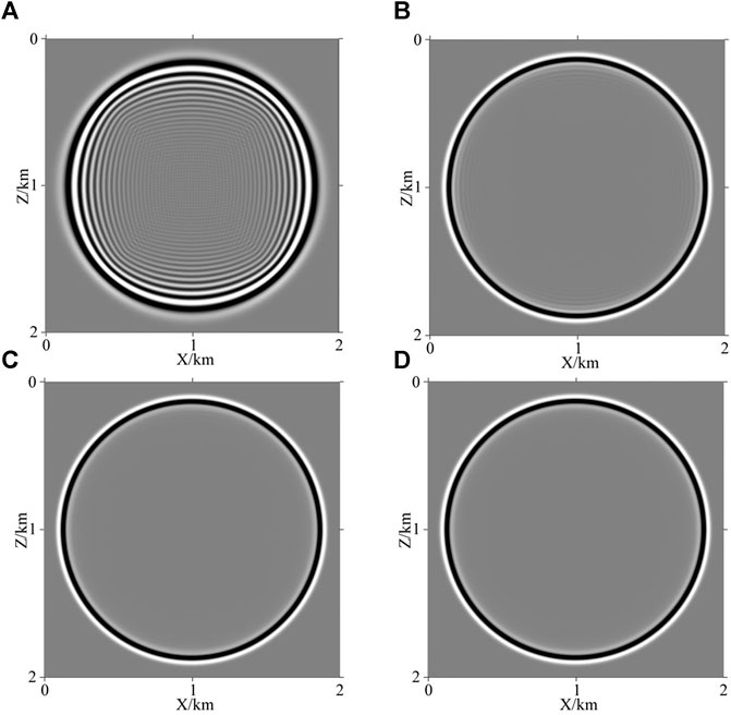
FIGURE 3. Snapshots of wavefield extrapolation based on different orders of finite-difference operator in a pseudo-space-domain difference expression (A), (B), (C), and (D) correspond, respectively, to second-order, eighth-order, twelfth-order, and sixteenth-order.

It can be seen from the snapshot shown in Figure 3 that, for the pseudo-space-domain FD scheme with different orders of FD operator, when the spatial grid interval, model velocity, and wavelet dominant frequency are the same, the higher the order of FD operator is, the weaker the dispersion is.

Stability Condition for the Pseudo-Space-Domain First-Order Velocity-Stress Acoustic Wave Equation

First, we define the pseudo-space-domain plane harmonic variables $u$

$u=u_0{e}^{i\omega n\Delta t}{e}^{i{k}_{{\tau }_x}j\Delta {\tau }_x}{e}^{i{k}_{{\tau }_z}k\Delta {\tau }_z},(14)$

where $u_0$ represents the initial wavefield, $\omega$ represents the circular frequency, $k_{{\tau }_x}$ and $k_{{\tau }_z}$ represent wave numbers in the ${\tau }_x$ and ${\tau }_z$ directions, respectively; $n$, $j$, and $k$ represent coordinates of discrete grid points in the $t$, ${\tau }_x$, and ${\tau }_z$ directions, respectively; $\Delta {\tau }_x$ and $\Delta {\tau }_z$represent pseudo-space-domain intervals in the ${\tau }_x$ and ${\tau }_z$ directions, respectively; $e$ stands for the base of the natural logarithms, and $i$ represents the imaginary unit in this section. According to the above equation, one can get the following relationships:

$\{\begin{array}{l}{u}_{{\tau }_x+\Delta {\tau }_x^{+m}}=u_{{\tau }_x}{e}^{i{k}_{{\tau }_x}\Delta {\tau }_x^{+m}},\\ u_{{\tau }_x-\Delta {\tau }_x^{-m}}=u_{{\tau }_x}{e}^{-i{k}_{{\tau }_x}\Delta {\tau }_x^{-m}}.\end{array}(15)$

Substituting the above formulas into the first-derivative difference expression gives

$\frac{du}{d{\tau }_x}=u{\displaystyle \sum _{m=1}^N\left(c_{2m-1}^x{e}^{i{k}_{{\tau }_x}\Delta {\tau }_x^{+m}}+c_{2m}^x{e}^{-i{k}_{{\tau }_x}\Delta {\tau }_x^{-m}}\right)}.(16)$

Furthermore, the second-derivative expression for ${\tau }_x$ can be obtained as

$\frac{d^{2}u}{d{\tau }_x^2}=u{\left\{{\displaystyle \sum _{m=1}^N\left(c_{2m-1}^x{e}^{i{k}_{{\tau }_x}\Delta {\tau }_x^{+m}}+c_{2m}^x{e}^{-i{k}_{{\tau }_x}\Delta {\tau }_x^{-m}}\right)}\right\}}^2.(17)$

According to the definition of the propagation time in the pseudo-space-domain and the sampling theorem, when the maximum wave number for ${\tau }_x$ is obtained, the following relationships hold: $\Delta {\tau }_x^{+m}{k}_{{\tau }_x}=\left(m-1/2\right)\pi$ and $\Delta {\tau }_x^{-m}{k}_{{\tau }_x}=\left(m-1/2\right)\pi$. Therefore, the above equation can be converted into

$\frac{d^{2}u}{d{\tau }_x^2}=-u{\left\{{\displaystyle \sum _{m=1}^N\left({\left(-1\right)}^{m-1}{c}_{2m-1}^x+{\left(-1\right)}^m{c}_{2m}^x\right)}\right\}}^2.(18)$

Similarly, the second-derivative expression for ${\tau }_z$ can be obtained as

$\frac{d^{2}u}{d{\tau }_z^2}=-u\left\{{\displaystyle \sum _{m=1}^N\left({\left(-1\right)}^{m-1}{c}_{2m-1}^z+{\left(-1\right)}^m{c}_{2m}^z\right)}\right\}{,}^2(19)$

and the second-derivative expression for $t$ can be obtained as

$\frac{{\partial }^{2}u}{\partial t^2}=-u{\left(\frac{2\sin \left(\omega \Delta t/2\right)}{\Delta t}\right)}^2(20)$

Eq. (4) is reduced to the form of a pseudo-space-domain second-order scalar acoustic wave equation, and Eqs. (18), (19), and (20) are substituted to yield

${\left(\frac{2\sin \left(\omega \Delta t/2\right)}{\Delta t}\right)}^2={\left\{{\displaystyle \sum _{m=1}^N\left({\left(-1\right)}^{m-1}{c}_{2m-1}^x+{\left(-1\right)}^m{c}_{2m}^x\right)}\right\}}^2+{\left\{{\displaystyle \sum _{m=1}^N\left({\left(-1\right)}^{m-1}{c}_{2m-1}^z+{\left(-1\right)}^m{c}_{2m}^z\right)}\right\}}^2.(21)$

Because the left side of the equation above satisfies $0\le {\sin }^2\omega \frac{\Delta t}{2}\le 1$, and under the assumption that the differential coefficients in the ${\tau }_x$ and ${\tau }_z$ directions are equal, the following relation holds:

$\Delta t\le \frac{\sqrt{2}}{\left|{\displaystyle \sum _{m=1}^N\left({\left(-1\right)}^{m-1}{c}_{2m-1}+{\left(-1\right)}^m{c}_{2m}\right)}\right|},(22)$

where $c_m=c_m^x=c_m^z$ $\left(m=\mathrm{1,2},\dots ,2N-\mathrm{1,2}N\right)$.

Perfectly Matched Layer Boundary Conditions of the Pseudo-Space-Domain First-Order Velocity-Stress Acoustic Wave Equation

In the central wavefield calculation region, FD numerical simulation of the pseudo-space-domain first-order velocity-stress acoustic wave equation with 2Nth order in pseudo-space and second-order in time can be realized by applying Eq. 13. In the artificial boundary region, to effectively suppress the artificial boundary reflection, absorbing boundary processing is required. The perfectly matched layer (PML) boundary conditions for the first-order velocity-stress acoustic wave equation in the pseudo-space-domain are given below.

Because the PML attenuation term is independent of the partial derivative of wave equation, the space domain partial derivative in the equation is transformed into a pseudo-space-domain partial derivative; meanwhile, the space domain attenuation factors $d_x$ and $d_z$ are transformed into pseudo-space-domain attenuation factors $d_{{\tau }_x}$ and $d_{{\tau }_z}$. The PML boundary conditions for the pseudo-space-domain acoustic wave equation are as follows:

$\{\begin{array}{l}\frac{\partial v_x}{\partial t}+d_{{\tau }_x}{v}_x=-\frac{1}{\rho }\frac{\partial P}{\partial {\tau }_x},\\ \frac{\partial v_z}{\partial t}+d_{{\tau }_z}{v}_z=-\frac{1}{\rho }\frac{\partial P}{\partial {\tau }_z},\\ \frac{\partial P_x}{\partial t}+d_{{\tau }_x}{P}_x=-\rho \frac{\partial v_x}{\partial {\tau }_x},\\ \frac{\partial P_z}{\partial t}+d_{{\tau }_z}{P}_z=-\rho \frac{\partial v_z}{\partial {\tau }_z},\\ P=P_x+P_z,\end{array}(23)$

where $P_x$ and $P_z$ represent the components of $P$ in the ${\tau }_x$ and ${\tau }_z$ directions. $d_{{\tau }_x}$ and $d_{{\tau }_z}$ represent the attenuation factors in the ${\tau }_x$ and ${\tau }_z$ directions, which are given by

$d\left({\tau }_m\right)=\log \left(\frac{1}{R}\right)\cdot \frac{3}{2{\tau }_L}{\left(\frac{{\tau }_m}{{\tau }_L}\right)}^2,(24)$

where ${\tau }_m$ represents the normal pseudo-space-domain propagation time interval from the point in the PML layer to the outer edge of the center wavefield, $R$ represents the theoretical reflection coefficient for the PML layer (ranging from 10^–5 to 10^–7), and ${\tau }_L$ represents the pseudo-space-domain PML layer thickness. As is shown in Figure 4, when wavefield calculations are performed, $d_{{\tau }_x}=0$, $d_{{\tau }_z}=0$ in the center wavefield area; $d_{{\tau }_x}=0$, $d_{{\tau }_z}=d\left({\tau }_m\right)$ in PML areas one and PML area 4; $d_{{\tau }_x}=d\left({\tau }_m\right)$, $d_{{\tau }_z}=0$ in PML areas two and PML area three; and $d_{{\tau }_x}=d\left({\tau }_m\right)$, $d_{{\tau }_z}=d\left({\tau }_m\right)$ in the corner area.

FIGURE 4

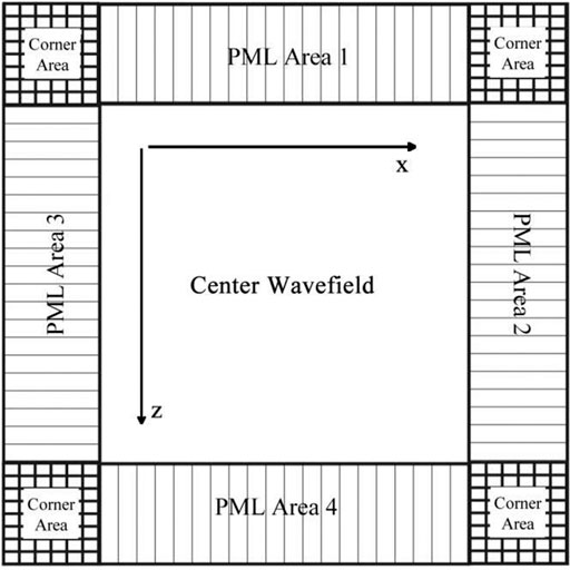
FIGURE 4. PML layer distribution diagram (Zhang et al., 2016).

We can write the attenuation factors $d_{{\tau }_x}{v}_x$, $d_{{\tau }_z}{v}_z$, $d_{{\tau }_x}{P}_x$, and $d_{{\tau }_z}{P}_z$ in the PML boundary conditions into a differential form, and by substituting them with the difference expression of each first-order derivative into Eq. 23, we can derive

$\{\begin{array}{l}{v}_{x{\tau }_{i+1/2},{\tau }_j}^{k+1/2}=\frac{1}{1+d_{{\tau }_x}\Delta t/2}[\left(1-d_{{\tau }_x}\Delta t/2\right)v_{x{\tau }_{i+1/2},{\tau }_j}^{k-1/2}\\ -\frac{\Delta t}{\rho }{\displaystyle \sum _{m=1}^N\left(c_{2m-1}^x{P}_{{\tau }_{i+1/2}+\Delta {\tau }_{i+1/2}^{+m},{\tau }_j}^k+c_{2m}^x{P}_{{\tau }_{i+1/2}-\Delta {\tau }_{i+1/2}^{-\left(m-1\right)},{\tau }_j}^k\right)}],\\ v_{z{\tau }_i,{\tau }_{j+1/2}}^{k+1/2}=\frac{1}{1+d_{{\tau }_z}\Delta t/2}[\left(1-d_{{\tau }_z}\Delta t/2\right)v_{z{\tau }_i,{\tau }_{j_{+1/2}}}^{k-1/2}\\ -\frac{\Delta t}{\rho }{\displaystyle \sum _{m=1}^N\left(c_{2m-1}^z{P}_{{\tau }_i,{\tau }_{j+1/2}+\Delta {\tau }_{i+1/2}^{+m}}^k+c_{2m}^z{P}_{{\tau }_i,{\tau }_{j+1/2}-\Delta {\tau }_{j+1/2}^{-\left(m-1\right)}}^k\right)}],\\ P_{x{\tau }_i,{\tau }_j}^{k+1}=\frac{1}{1+d_{{\tau }_x}\Delta t/2}[\left(1-d_{{\tau }_x}\Delta t/2\right)P_{x{\tau }_i,{\tau }_j}^k\\ -\rho \Delta t{\displaystyle \sum _{m=1}^N\left(c_{v2m-1}^x{v}_{x{\tau }_i+\Delta {\tau }_i^{+\left(m-1/2\right)},{\tau }_j}^{k+1/2}+c_{v2m}^x{v}_{x{\tau }_i-\Delta {\tau }_i^{-\left(m-1/2\right)},{\tau }_j}^{k+1/2}\right)}],\\ P_{z{\tau }_i,{\tau }_j}^{k+1}=\frac{1}{1+d_{{\tau }_z}\Delta t/2}[\left(1-d_{{\tau }_z}\Delta t/2\right)P_{z{\tau }_i,{\tau }_j}^k\\ -\rho \Delta t{\displaystyle \sum _{m=1}^N\left(c_{v2m-1}^z{v}_{x{\tau }_i,{\tau }_j+\Delta {\tau }_j^{+\left(m-1/2\right)}}^{k+1/2}+c_{v2m}^z{v}_{x{\tau }_i,{\tau }_j-\Delta {\tau }_j^{-\left(m-1/2\right)}}^{k+1/2}\right)}],\\ P_{{\tau }_i,{\tau }_j}^{k+1}=P_{x{\tau }_i,{\tau }_j}^{k+1}+P_{z{\tau }_i,{\tau }_j}^{k+1}.\end{array}(25)$

Equation 25 is the difference expression for PML boundary conditions of the pseudo-space-domain first-order velocity-stress acoustic wave equation.

A uniform medium model is used to verify the effectiveness of the PML boundary conditions of first-order velocity-stress acoustic wave equations in the pseudo-space-domain for eliminating artificial boundary reflections. The horizontal and vertical lengths of the model are 2000 and 2000 m, respectively, and the grid interval is 5 m. The primary wave velocity in the model is 2,500 m/s, and the density is 2000 kg/m³. The source location is (1,000 m, 1,000 m), and the source wavelet employs Ricker wavelet with a dominant frequency of 35 Hz. To avoid the effects of numerical dispersion, the pseudo-space-domain FD order is 10th order. The snapshot of the wavefield extrapolation process at 0.82 s is shown in Figure 5, where Figure 5A shows the snapshot of the left boundary without the PML boundary conditions, and Figure 5B shows a snapshot of the left boundary with PML boundary conditions.

FIGURE 5

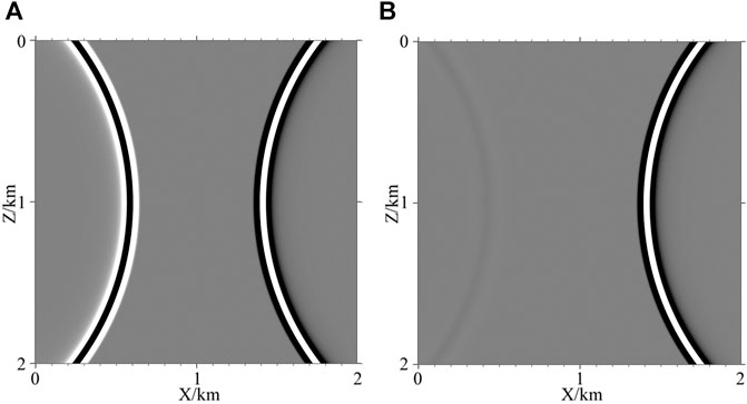
FIGURE 5. Snapshot of the pseudo-space-domain acoustic wave equation at 0.82 s: (A) left boundary without PML boundary conditions; (B) left boundary with PML boundary conditions.

To further illustrate the boundary absorption effect of the PML boundary conditions in the pseudo-space-domain acoustic wave equation, the left boundary reflection wave corresponding to a depth of 1 km in the wavefield shown in Figure 5 is magnified and displayed and is compared with the conventional acoustic wave equation wave based on the same simulation parameters. As shown in Figure 6, the black solid line is the left boundary reflection wave absorbed by the PML boundary condition of the pseudo-space-domain acoustic wave equation, the red dotted line is the left boundary reflection wave absorbed by the PML boundary condition of conventional method, and the blue dotted line is the reflected wave of left boundary without attenuation by PML boundary conditions. It can be seen that the amplitude of the boundary reflection wave after absorption by the pseudo-space-domain PML boundary condition is basically the same as that obtained by the conventional PML boundary condition, and it is obviously weaker than the amplitude of the uncompressed boundary reflection wave.

FIGURE 6

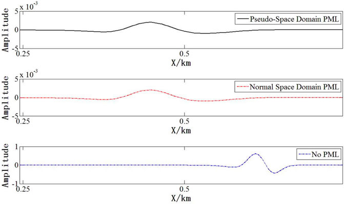
FIGURE 6. PML boundary condition absorption effect comparison.

Normalized Cross-Correlation Imaging Conditions

In this study, normalized cross-correlation imaging conditions (Kaelin and Guitton, 2006) are used in the RTM. The realization process employs the zero-delay cross-correlation of the source wavefield to normalize the zero-delay cross-correlation between the forward time wavefield and the reverse time wavefield as

$I\left(x,z\right)=\frac{{\displaystyle \sum _{t=0}^T{\left(v\right)}^F\left(x,z,t\right)\cdot {\left(v\right)}^R\left(x,z,t\right)}}{{\displaystyle \sum _{t=0}^T{\left(v\right)}^F\left(x,z,t\right)\cdot {\left(v\right)}^F\left(x,z,t\right)}},(26)$

where T is the total recording time. ${\left(v\right)}^F$ is the forward time wavefield, and ${\left(v\right)}^R$ is the reverse time wavefield.

When using the above imaging conditions, it is usually necessary to save the forward time wavefield at each time. However, when all the wavefield values are stored on the storage medium, large amount of memory storage space is required and also a long data access time. To overcome this problem, in this study, we implement an effective boundary storage strategy (Clapp, 2008; Wang et al., 2012) based on PML boundary conditions in the pseudo-space-domain. This entails storing the wavefield value of the N-layer grid point (the FD order is 2Nth order) that is adjacent to the central wavefield on each PML boundary during the forward time source wavefield extrapolation, as well as the central wavefield value at the last moment. These boundary wavefield values are taken out as a boundary condition when extrapolating along reverse time, and then, the source wavefield can be rebuilt in the time iteration. Although this method requires the forward time source wavefield extrapolation in advance, this can effectively reduce the storage requirements for the RTM in pseudo-space-domain.

Model Experiment

Reverse Time Migration of the Dipping Interface Model

The main purpose of this experiment is to test the validity of pseudo-space-domain acoustic wave equation RTM in solving velocity interface distortion and suppressing false scattering and reflected waves.

The experiment used a two-layer velocity model with a dipping interface, as shown in Figure 7A. The horizontal and vertical lengths were 4,000 m and 2000 m, respectively. The primary wave velocities at the upper and lower sides of the interface were 2,500 m/s and 3,500 m/s, respectively. The density was 2000 kg/m³. The grid model obtained by meshing this interface model with vertical and horizontal grid intervals of 10 m is shown in Figure 7B. It can be seen that the original smooth velocity interface has become an obviously stepped interface (white arrow in the figure). In the experiment, a geometry with a fixed position of receivers and changeable source position was established. The shot point was between 500 and 3,480 m, the interval between the shots was 20 m, and a total of 150 shots was made. There were 401 receivers per shot, and each receiver was located between 0 and 4,000 m. The interval between receivers was 10 m. The depths of shots and receivers were both 10 m.

FIGURE 7

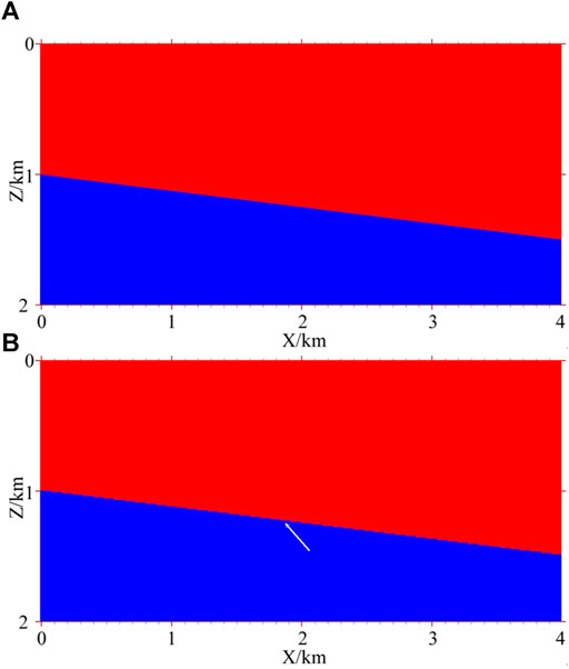
FIGURE 7. Two-layer velocity model with a dipping interface: (A) original model with a smooth dipping interface; (B) model with 10 m grid interval.

Obviously, to verify the effectiveness of a migration method in solving velocity interface distortion, it is necessary to ensure that the acquired seismic record is accurate. The shot records required for this experiment were obtained by using FD wave equation forward modeling. In theory, only by using a small enough grid spacing can ensure that the obtained shot records are relatively accurate. Therefore, in this study, we first used a model with 1 m grid intervals in both vertical and horizontal directions for forward modeling. (Note that, even if the number of grid points is only doubled, this can cause a huge increase in the amount of computation. Therefore, regardless of whether one realizes forward modeling in actual processing or migration and inversion, it is generally unrealistic to use such a small grid interval.) The simulation used a Ricker wavelet with a dominant frequency of 35 Hz. The FD order was 16th order in space and second-order in time, and a total of 150 shots of seismic records was obtained. The record of the 76th shot is shown in Figure 8A. For comparison, a record obtained with the grid interval of 10 m is shown in Figure 8B, which existed strong artificial scattered waves.

FIGURE 8

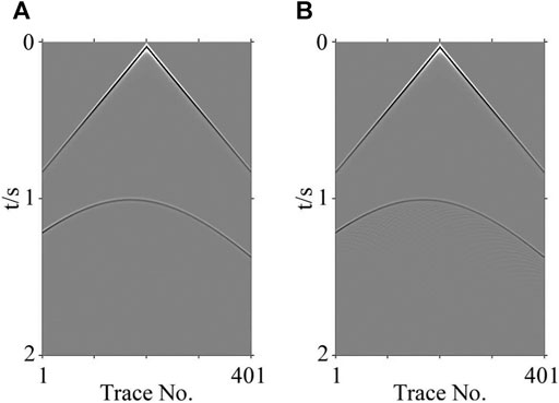
FIGURE 8. Synthetic shot gather record (76th shot ): (A) grid interval of 1 m; (B) grid interval of 10 m.

Based on the model of 10 m grid interval as shown in Figure 7B, the FD algorithm for the conventional and pseudo-space-domain acoustic wave equations is used for RTM with second-order accuracy in time and sixteenth-order accuracy in both space and pseudo-space. (Note that the pseudo-space-domain RTM needs to add velocity interface information to calculate the traveltime between two grid points.) The migration profiles are, respectively, shown in Figures 9A,B.

FIGURE 9

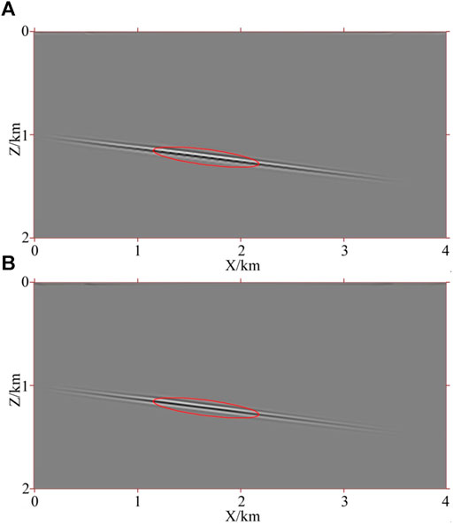
FIGURE 9. Reverse time migration seismic profile. (A) based on the conventional acoustic equation and (B) based on the pseudo-space-domain acoustic equation.

To more intuitively compare the morphology of the dipping interface in the migration profile of the two methods, the event in the elliptical region in Figures 9A,B is magnified, as shown in Figures 10A,B. It can be seen that the shape of the dipping interface in the RTM profile of the conventional acoustic wave equation (the red dotted line in Figure 10A) is significantly distorted compared with the real interface morphology (the red solid line in Figure 10A). The interface shape in the RTM profile of the pseudo-space-domain acoustic wave equation is basically consistent with the real interface morphology (the red solid line in Figure 10B). This demonstrates that pseudo-space-domain acoustic wave equation RTM can effectively solve the distortion problem of the velocity interface.

FIGURE 10

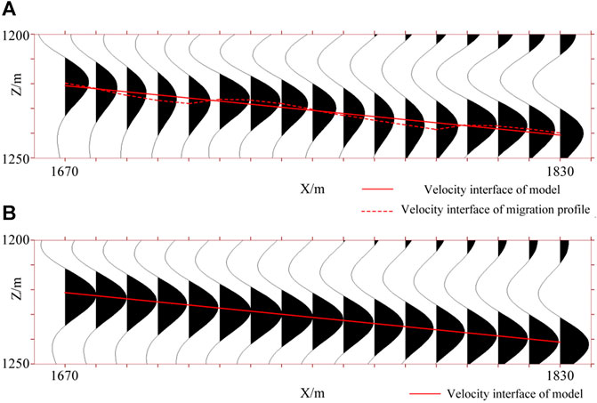
FIGURE 10. Local magnification of a reverse time migration profile. (A) based on the conventional acoustic equation and (B) based on the pseudo-space-domain acoustic equation.

Figures 11A,B show a snapshot of the forward time wavefield of the 76th shot at 0.9 s. It can be seen that there are obvious false scatterings in the wavefield of the conventional acoustic wave equation (as shown in the elliptical region in Figure 11A), and there are no obvious false scatterings in the wavefield of the pseudo-space-domain acoustic wave equation (as shown in the elliptical region in Figure 11B). By comparing the interface reflections at the arrows in Figure 11, we can see that the pseudo-space-domain acoustic wave equation significantly suppresses reflected waves (especially those of near-normal incidence). This demonstrates the effectiveness of the pseudo-space-domain acoustic wave equation in suppressing interfacial false scattering and reflected waves.

FIGURE 11

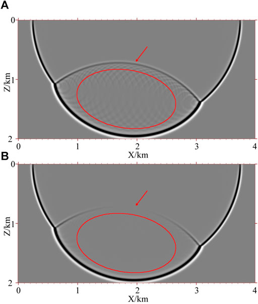
FIGURE 11. Snapshots of forward time wavefield in reverse time migration (76th shot at 0.9 s). (A) based on the conventional acoustic equation and (B) based on the pseudo-space-domain acoustic equation.

Reverse Time Migration of the Marmousi Model

The Marmousi model (shown in Figure 12) is a grid velocity model of complex tectonic with numerous velocity interfaces, steep dip structures, and dramatic velocity changes. The model size is 9,200 m * 3,000 m, respectively. The horizontal and vertical grid spacings are, respectively, 5 and 4 m. In the experiment, the unilateral shot geometry used was a seismic source located at the right side and receivers located at the left side. The interval between the shots was 25 m, with 426 shots in total. There were 104 receivers per shot. The depths of the shot and the receivers were both 8 m. The source wavelet used a Ricker wavelet with a dominant frequency of 35 Hz. Synthetic seismograms were simulated by the conventional acoustic wave equation FD method whose FD order was second-order in time and eighth-order in space.

FIGURE 12

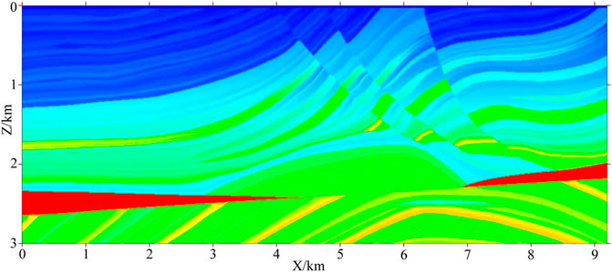
FIGURE 12. Grid velocity model of Marmousi.

We applied the conventional acoustic wave equation and pseudo-space-domain acoustic wave equation FD (with FD order being second-order in time and eighth-order in space and pseudo-space) to perform RTM. Figures 13A,B show the snapshots of the 138th shot based on the two methods at 1.9 s. Figures 14A,B show the RTM profiles based on the two methods, respectively.

FIGURE 13

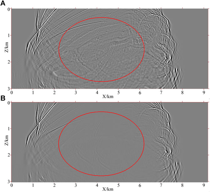
FIGURE 13. Forward time wavefield snapshots in reverse time migration for the Marmousi model (138th shot at 1.9 s in time). (A) based on the conventional acoustic equation and (B) based on the pseudo-space-domain acoustic equation.

FIGURE 14

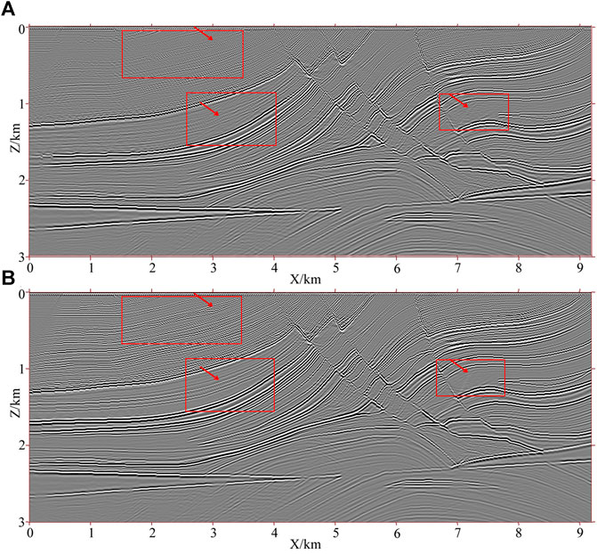
FIGURE 14. Reverse time migration profile for the Marmousi model. (A) based on the conventional acoustic equation and (B) based on the pseudo-space-domain acoustic equation.

Figure 13 shows that the pseudo-space-domain acoustic wave equation has a significantly weakened reflection wave in the wavefield compared with the conventional acoustic wave equation. It indicates the validity of the pseudo-space-domain acoustic wave equation in suppressing reflected waves during wavefield extrapolation.

Comparing the local migration profiles in the red rectangular region in Figure 14, we can see that the pseudo-space-domain acoustic wave equation has a clearer structure and better continuity of the event where the arrows point the conventional acoustic wave equation. This demonstrates that the imaging quality of RTM by using the pseudo-space-domain acoustic wave equation is better than that obtained by using a conventional acoustic wave equation.

Conclusion and Discussion

Based on the first-order velocity-stress acoustic wave equation in the pseudo-space-domain, we derived a 2Nth-order-accuracy staggered-grid FD expression and its PML boundary condition, deduced the stability conditions of the staggered-grid FD expression, and realized RTM in the pseudo-space-domain. At the same time, numerical experiments were carried out based on a dipping interface model and the Marmousi model. Experimental results were as follows:

1) The RTM method based on the pseudo-space-domain acoustic wave equation could solve the problem of velocity interface distortion that appears in the conventional RTM profile.

2) Wavefield extrapolation based on the pseudo-space-domain acoustic wave equation could significantly weaken interface false scattering and reflection waves, thereby further improving the quality of the migration imaging.

Of course, the high-order FD RTM method for the acoustic wave equations in the pseudo-space-domain is not ideal for reflection waves suppression under non-normal incidence. Therefore, the focus of future research work will be the further improvement of the reflection waves suppression effect of the method and accuracy of RTM imaging, along with developing it into the elastic wave equation and the RTM of the three-dimensional wave equation.

Data Availability Statement

The raw data supporting the conclusion of this article will be made available by the authors, without undue reservation.

Author Contributions

XZ: writing—original draft. XW: conceptualization, project administration. BL: suggestions. PS: formal analysis. JT: software. CX: methodology.

Funding

The authors are grateful for the support of the Shandong Provincial Natural Science Foundation (No. ZR2020QD071), the National Natural Science Foundation of China (No. 42106072; No. 42074138; No.U2006202), the Fundamental Research Funds for the Central Universities (No. 201964016), the Major Scientific and Technological Innovation Project of Shandong Province (No. 2019JZZY010803), and the Taishan Scholar Project Funding (No. tspd20161007).

Conflict of Interest

The authors declare that the research was conducted in the absence of any commercial or financial relationships that could be construed as a potential conflict of interest.

Publisher’s Note

All claims expressed in this article are solely those of the authors and do not necessarily represent those of their affiliated organizations, or those of the publisher, the editors, and the reviewers. Any product that may be evaluated in this article, or claim that may be made by its manufacturer, is not guaranteed or endorsed by the publisher.

References

Baysal, E., Kosloff, D. D., and Sherwood, J. W. C. (1984). A Two‐way Nonreflecting Wave Equation. Geophysics. 49 (2), 132–141. doi:10.1190/1.1441644

CrossRef Full Text | Google Scholar

Chang, W. F., and McMechan, G. A. (1987). Elastic Reverse‐Time Migration. Geophysics. 52 (10), 1365–1375. doi:10.1190/1.1442249

CrossRef Full Text | Google Scholar

Chang, W.-F., and McMechan, G. A. (1990). 3D Acoustic Prestack Reverse-Time Migration1. Geophys. Prospect. 38 (7), 737–755. doi:10.1111/j.1365-2478.1990.tb01872.x

CrossRef Full Text | Google Scholar

Chang, W. F., and McMechan, G. A. (1994). 3-D Elastic Prestack, Reverse‐Time Depth Migration. Geophysics. 59 (4), 597–609. doi:10.1190/1.1443620

CrossRef Full Text | Google Scholar

Chu, C. L., and Wang, X. T. (2005). Seismic Modeling With a Finite-Difference Method on Irregular Triangular Grids. Periodical Ocean Univ. China. 35 (01), 43–48. doi:10.16441/j.cnki.hdxb.2005.01.0.09

CrossRef Full Text | Google Scholar

Clapp, R. G. (2008). Reverse Time Migration: Saving the Boundaries. Stanford Exploration Project Tech. Rep. 136, 136–144.

Google Scholar

Clapp, R. G. (2009). Reverse Time Migration with Random Boundaries. 79th Annu. Int. Meet. (Houston: SEG Expanded Abstract), 2809–2813. doi:10.1190/1.3255432

CrossRef Full Text | Google Scholar

Du, Q. Z., Zhu, Y. T., Zhang, M. Q., and Gong, X. F. (2013). A Study on the Strategy of Low Wavenumber Noise Suppression for Prestack Reverse-Time Depth Migration. Chin. J. Geophys. 56 (7), 2391–2401. doi:10.6038/cjg20130725

CrossRef Full Text | Google Scholar

He, B. S., Zhang, H. X., and Zhang, J. (2008). Prestack Reverse-Time Depth Migration of Arbitrarily Wide-Angle Wave Equations. Acta Seismologica Sinica. 30 (5), 491–499. doi:10.3321/j.issn:0253-3782.2008.05.007

CrossRef Full Text | Google Scholar

Huang, C., and Dong, L. G. (2009). High-Order FD Method in Seismic Wave Simulation With Variable Grids and Local Time-Steps. Chin. J. Geophys. 52 (11), 176–186. doi:10.3969/j.issn.0001-5733.2009.11.022

CrossRef Full Text | Google Scholar

Kaelin, B., and Guitton, A. (2006). Imaging Condition for Reverse Time Migration. 76th Annu. Int. Meet. (New Orleans: SEG Expanded Abstract), 2594–2598. doi:10.1190/1.2370059

CrossRef Full Text | Google Scholar

Lan, H., Zhang, Z., Chen, J., and Liu, Y. (2014). Reverse Time Migration from Irregular Surface by Flattening Surface Topography. Tectonophysics. 627, 26–37. doi:10.1016/j.tecto.2014.04.015

CrossRef Full Text | Google Scholar

Li, H., Li, J., Gu, N., Gao, J., and Zhang, H. (2020). Ambient Noise Surface Wave Reverse Time Migration for Fault Imaging. J. Geophys. Res. Solid Earth. 125, e2020JB020381. doi:10.1029/2020JB020381

CrossRef Full Text | Google Scholar

Li, Y., Choi, Y., Alkhalifah, T., Li, Z., and Zhang, K. (2018). Full-Waveform Inversion Using a Nonlinearly Smoothed Wavefield. Geophysics. 83 (2), R117–R127. doi:10.1190/geo2017-0312.1

CrossRef Full Text | Google Scholar

Liu, F., Zhang, G., Morton, S. A., and Leveille, J. P. (2011). An Effective Imaging Condition for Reverse-Time Migration Using Wavefield Decomposition. Geophysics. 76 (1), S29–S39. doi:10.1190/1.3533914

CrossRef Full Text | Google Scholar

Liu, H. W., Li, B., Liu, H., Tong, X. L., and Liu, Q. (2010). The Algorithm of High Order Finite Difference Pre-stack Reverse Time Migration and GPU Implementation. Chin. J. Geophys. 53 (7), 600–610. doi:10.1002/cjg2.1530

CrossRef Full Text | Google Scholar

Liu, Q., Zhang, J., and Gao, H. (2016). Reverse-Time Migration From Rugged Topography Using Irregular, Unstructured Mesh. Geophys. Prospecting. 65 (2), 453–466. doi:10.1111/1365-2478.12415

CrossRef Full Text | Google Scholar

Liu, Q., and Zhang, J. (2020). Topography Least-Squares Reverse-Time Migration Based on Adaptive Unstructured Mesh. Surv. Geophys. 41, 343–361. doi:10.1007/s10712-019-09578-0

CrossRef Full Text | Google Scholar

Liu, X. X., Yin, X. Y., and Liu, B. H. (2013). Prestack Reverse Time Migration of Elastic Waves in Porous media. Prog. Geophys. 28 (6), 3165–3173. doi:10.6038/pg20130643

CrossRef Full Text | Google Scholar

McMechan, G. A. (1983). Migration by Extrapolation of Time-dependent Boundary Values. Geophys. Prospect. 31 (3), 413–420. doi:10.1111/j.1365-2478.1983.tb01060.x

CrossRef Full Text | Google Scholar

Moradpouri, F., Moradzadeh, A., Pestana, R., Ghaedrahmati, R., and Soleimani Monfared, M. (2017). An Improvement in Wavefield Extrapolation and Imaging Condition to Suppress Reverse Time Migration Artifacts. Geophysics. 82 (6), S403–S409. doi:10.1190/geo2016-0475.1

CrossRef Full Text | Google Scholar

Qu, Y., Guan, Z., and Li, Z. (2019). Topographic Elastic Least‐squares Reverse Time Migration Based on Vector P‐ and S‐wave Equations in the Curvilinear Coordinates. Geophys. Prospecting. 67 (5), 1271–1295. doi:10.1111/1365-2478.12775

CrossRef Full Text | Google Scholar

Shi, Y., Ke, X., and Zhang, Y. Y. (2015). Analyzing the Boundary Conditions and Storage Strategy for Reverse Time Migration. Prog. Geophys. 30 (2), 581–585. doi:10.6038/pg20150214

CrossRef Full Text | Google Scholar

Shragge, J. (2014). Reverse Time Migration from Topography. Geophysics. 79 (4), S141–S152. doi:10.1190/GEO2013-0405.1

CrossRef Full Text | Google Scholar

Song, P. (2005). Accurate Absorbing Boundary Conditions and Reverse-Time Migration of Acoustic Wave Equation Using Non-reflecting Recursive Algorithm: [Master’s Thesis]. Qingdao: Ocean University of China.

Google Scholar

Song, P., Zhu, B., Li, J. S., and Tan, J. (2015). Reverse Time Migration of Divided-Order Multiples. Chin. J. Geophys. 58 (10), 3791–3803. doi:10.6038/cjg20151029

CrossRef Full Text | Google Scholar

Sun, R., and McMechan, G. A. (2001). Scalar Reverse‐Time Depth Migration of Prestack Elastic Seismic Data. Geophysics. 66 (5), 1519–1527. doi:10.1190/1.1487098

CrossRef Full Text | Google Scholar

Virieux, J. (1984). SH-Wave Propagation in Heterogeneous Media: Velocity‐Stress Finite‐Difference Method. Geophysics. 49 (11), 1933–1942. doi:10.1190/1.1441605

CrossRef Full Text | Google Scholar

Wang, B. L., Gao, J. H., Chen, W. C., and Zhang, H. L. (2012). Efficient Boundary Storage Strategies for Seismic Reverse Time Migration. Chin. J. Geophys. 55 (07), 2412–2421. doi:10.6038/j.issn.0001-5733.2012.07.025

CrossRef Full Text | Google Scholar

Wang, X., Xia, D., Li, J., Tang, Q., and Jiang, X. (2005). Model Based Processing (III): Pseudo‐Space Reverse Time Migration. 75th Annu. Int. Meet. (Houston: SEG Expanded Abstract), 1838–1841. doi:10.1190/1.2148060

CrossRef Full Text | Google Scholar

Whitmore, N. D. (1983). Iterative Depth Migration by Backward Time Propagation. 53rd Annu. Int. Meet. (Las Vegas: SEG Expanded Abstract), 382–386. doi:10.1190/1.1893867

CrossRef Full Text | Google Scholar

Willacy, C., and Kryvohuz, M. (2019). Reverse Time Migration of Transmitted Wavefields for Salt Boundary Imaging. Geophysics. 84 (2), S71–S82. doi:10.1190/geo2018-0182.1

CrossRef Full Text | Google Scholar

Yan, H. Y. (2012). Study on Seismic Wave Field Numerical Simulation and Prestack Reverse Time Migration Method in Viscoelastic Medium: [PhD Thesis]. Beijing: China University of Petroleum.

Google Scholar

Yoon, K., and Marfurt, K. J. (2006). Reverse-Time Migration Using the Poynting Vector. Exploration Geophys. 37 (1), 102–107. doi:10.1071/EG06102

CrossRef Full Text | Google Scholar

Zhang, H. X., and Ning, S. N. (2002). Pre-Stack Reverse Time Migration of Elastic Wave Equation. J. China Univ. Mining Technology. 31 (5), 371–375. doi:10.3321/j.issn:1000-1964.2002.05.008

CrossRef Full Text | Google Scholar

Zhang, X. B., Song, P., Li, J. S., Tan, J., Liu, Z. L., and Xia, D. M. (2016). Analysis of the Impactof the Theoretical Reflection Coefficient on the Perfectly Matched Layer Absorbing Boundary. Periodical of Ocean University of China. 46 (06), 84–89. doi:10.16441/j.cnki.hdxb.20150190

CrossRef Full Text | Google Scholar

Zhou, H. W., Hu, H., Zou, Z., Wo, Y., and Youn, O. (2018). Reverse Time Migration: a Prospect of Seismic Imaging Methodology. Earth-Science Rev. 179 (2018), 207–227. doi:10.1016/j.earscirev.2018.02.008

CrossRef Full Text | Google Scholar

Zhu, S. W., Qu, S. L., Wei, X. C., and Liu, C. Y. (2007). Numeric Simulation by Grid-Various Finite-Difference Elastic Wave Equation. Oil Geophys. Prospecting. 42 (06), 634–639. doi:10.3321/j.issn:1000-7210.2007.06.006

CrossRef Full Text | Google Scholar

Zhu, S. W., and Wei, X. C. (2005). Differential Forward Modeling of Wave Equation Having Irregular Grid and Any-Order Precision. Oil Geophys. Prospecting. 40 (02), 149–153. doi:10.3321/j.issn:1000-7210.2005.02.012

CrossRef Full Text | Google Scholar