The Pseudo-Laplace Filter for Vector-Based Elastic Reverse Time Migration

The scalar images (PP and PS) can be effectively obtained in vector-based elastic reverse time migration by applying dot product–based scalar imaging conditions to the separated vector wavefields. However, the PP image suffers from polarity reversal issues when opening angles are greater than $\mathrm{9}{\mathrm{0}}^{\circ }$ and backscattering artifacts when opening angles are close to $\mathrm{18}{\mathrm{0}}^{\circ }$. To address these issues, we propose the pseudo-Laplace filter for the dot product–based scalar imaging condition. Based on the analysis of the Laplace filter in the scalar image of vector-based wavefields, the second-order parallel-oriented partial derivatives of Cartesian components cross-correlation results are selected to construct the pseudo-Laplace filter. In contrast, second-order normal-oriented partial derivatives of the Cartesian component’s cross-correlation results are omitted. The theoretical analysis with the plane wave assumption shows that the proposed pseudo-Laplace filter can solve the problems of backscattering artifacts and polarity reversal in PP images by the scalar imaging condition. Due to additional polarity correction and backscattering attenuation, numerical examples show excellent performance in PP images with a pseudo-Laplace filter. Furthermore, the application of the pseudo-Laplace filter requires trivial additional computation or storage.

Introduction

Reverse time migration (RTM) is a seismic data processing method for migrating seismic reflection data to obtain subsurface images that effectively describe geological structures (Baysal et al., 1983; McMechan, 1983; Whitmore, 1983). Multicomponent seismic data processing techniques have been evolved with seismic acquisition techniques and high-performance computing technologies to acquire more precise images. Elastic reverse time migration (elastic RTM) is one of the most reliable multicomponent seismic data imaging techniques that can provide surface PP and PS reflection information using P-wave and S-wave reflection data. Unlike acoustic RTM, which analyzes P-wave propagation in the subsurface medium, elastic RTM integrates elastic P-wave and S-wave propagation with wave conversion. As a result, the wave conversion-related elastic response and vector-based propagation characteristics are more accurate than the acoustic approximation.

Like acoustic RTM, the early elastic RTM (Sun and McMechan, 1986) used elastic wave equation to forward and backward extrapolation wavefields and extract images by cross-correlation imaging conditions for Cartesian components. For these images, the migration results of different modes are intermixed together. The interference would result in crosstalks in final images and make it difficult to highlight the advantages of S-wave information. The S-wave information can be further used to supplement P-wave images in imaging targets with poor PP reflectivity or under gas clouds. Therefore, in addition to applying wavefield extrapolation and imaging conditions, a more suitable approach for elastic RTM to obtain decoupled elastic wavefield is wavefield separation. Early attempts of wavefield separation use divergence and curl operators. The P wave separated by a divergence operator is usually represented by a scalar-based wavefield, and the S wave separated by a curl operator is usually represented by a scalar-based wavefield in a 2D case or a vector-based wavefield in a 3D case. Their amplitude and phase are different from the original elastic wavefield. Recently, the decoupled wave equation approach has been proposed. The decoupled wave equations (Ma and Zhu, 2003; Li, 2007; Wang and McMechan, 2015; Du et al., 2017) have been proposed to decouple the wavefields of displacement or particle velocity. Zhu (2017) has used Helmholtz decomposition and vector Poisson’s equation to decompose P- and S-mode wavefields with correct phases, amplitudes, and physical units similar to the decoupled wave equation. Furthermore, the decoupled wave equation with the assumption of heterogeneous medium (Elita Li et al., 2018; Tang and McMechan, 2018) has also been proposed to handle the wavefield coupling problem at interfaces. The separated P wave and S wave are represented by vector-based wavefields and have the same amplitude and phase as the original elastic wavefield. Therefore, we apply the decoupled wave equations to construct the decoupled source and receiver wavefields.

In addition to wavefield separation, imaging conditions are also the key ingredient for the elastic RTM algorithm to determine the accuracy and quality of imaging results. According to different wavefield separation methods and wavefield representations, imaging conditions are also different. As for scalar-based P wave and vector-based S wave based on divergence and curl operators, various imaging conditions include cross-correlation imaging conditions or divergence- and curl-based imaging conditions (Yan and Sava, 2008; Du et al., 2014). As a result, the migrated PP image may encounter backscattering artifacts whose opening angle is near $\mathrm{18}{\mathrm{0}}^{\circ }$, and the migrated PS image may encounter a polarity reversal problem at the normal incident, which is caused by the sign change of the S wave from the curl operator on two sides of the normal incident. The Laplace filter (Youn and Zhou, 2001) could suppress backscattering noise in PP images with trivial computation and storage costs.

Furthermore, the S wave’s polarization by Poynting vector (Du et al., 2013) or the modified imaging condition (Duan and Sava, 2015) can correct the polarity reversal problem to a certain degree. As for the vector-based P wave and S wave by the decoupled wave equation, the scalar PP and PS images are required to facilitate further interpretation. There are some imaging conditions, such as the cross-correlation imaging condition of Cartesian components (Claerbout, 1971), the scalar imaging condition (Wang and McMechan, 2015; Du et al., 2017; Zhu, 2017; Yang et al., 2018), and energy cross-correlation imaging condition (Rocha et al., 2016). The cross-correlation imaging condition of Cartesian components generates multiple imaging results for interpretation, while the energy cross-correlation imaging condition only generates one image of elastic energy, which misses some important convert-wave information. Therefore, the dot product–based scalar imaging conditions, extended from cross-correlation imaging conditions and sum up these cross-correlation images of Cartesian components together, have been used to obtain the final scalar images (PP and PS).

The scalar imaging condition can output scalar images (PP and PS) of vector wavefields but an encounter with polarity reversal problem and backscattering artifacts in PP images. Different from the polarity reversal in the PS image in which P wave and S wave are separated by divergence and curl operators, the polarity reversal problem is introduced to PP images by scalar imaging conditions while the opening angle exceeds $\mathrm{9}{\mathrm{0}}^{\circ }$. Du et al. (2017) have used Poynting vectors to analyze the sign change of PP images by scalar imaging conditions versus opening angles. Then, Tang and McMechan (2018) have used Poynting vectors to extract their angle gathers to correct the polarity reversal. These methods, as mentioned above, can solve the polarity reversal problem and lead to a significant extra cost of computation and storage. As for the attenuation of backscattering noise, the angle attenuation factors (Yoon and Marfurt, 2006) and high-pass filters can be used to suppress the image of large opening angles. As a widely used approach, the high-pass filter is easy to implement. Among high-pass filters, the Laplace filter (Youn and Zhou, 2001) has successfully suppressed backscattering noise in PP images by cross-correlation imaging conditions.

In this article, based on the analysis of the Laplace filter in the vector-based scalar image, we select the parallel-oriented partial derivatives and abandon normal-oriented partial derivatives of the Cartesian component’s cross-correlation results to propose the pseudo-Laplace filter and produce an optimized image. Theoretical analysis with the plane wave assumption is then carried out to show that the PP image with a pseudo-Laplace filter succeeds in backscattering attenuation and polarity correction. Finally, the numerical experiments prove that the pseudo-Laplace filter can guarantee its stability and practicability without increasing additional computation burdens.

Methodology

The vector-based elastic RTM algorithms are as follows: 1) forward extrapolated decoupled source wavefields using the decoupled wave equation and retaining their boundary values at imaging time points; 2) back extrapolated decoupled receiver wavefields using the decoupled wave equation and reconstructing the source wavefields by the retained boundary values at the same imaging time point; 3) applying scalar imaging conditions to construct scalar imaging results (PP and PS). Here, we analyze the scalar imaging condition based on the decoupled wave equation and apply it using a Laplace filter or pseudo-Laplace filter.

The Decoupled Wave Equation

In a homogeneous and isotropic medium, the elastic wave extrapolation (Aki and Richards, 1980) can be expressed as follows:

$\rho \ddot{\mathbf{u}}=\left(\lambda +2\mu \right)\nabla \left(\nabla \cdot \mathbf{u}\right)-\mu \nabla \times \nabla \times \mathbf{u},\mathbf{ }(1)$

where $\mathbf{u}$ and $\ddot{\mathbf{u}}$ are the displacement vector wavefield and its second-order time derivative; $\lambda$, $\mu$ and $\rho$ are the Lame’s moduli and density, respectively. Based on the Helmholtz theorem (Dellinger and Etgen, 1990), the elastic wavefield in an isotropic case can be separated into a curl-free P wavefield $\left(\nabla \times {\mathbf{u}}_P=\mathbf{0}\right)$ and a divergence-free S wavefield $\left(\nabla \cdot {\mathbf{u}}_S=0\right)$. ${\mathbf{u}}_P$ and ${\mathbf{u}}_S$ are the P-wave and S-wave displacement vector wavefields. Analogous to the separation of displacement wavefield, the second-order time derivative of displacement wavefield can be decomposed as $\ddot{\mathbf{u}}={\ddot{\mathbf{u}}}_P+{\ddot{\mathbf{u}}}_S$, where

$\{\begin{array}{l}{\ddot{\mathbf{u}}}_P=\left(\lambda +2\mu \right)\nabla \left(\nabla \cdot \mathbf{u}\right)\hfill \\ \begin{array}{l}{\ddot{\mathbf{u}}}_S=-\mu \nabla \times \nabla \times \mathbf{u}\\ \mathbf{u}={\mathbf{u}}_P+{\mathbf{u}}_S\end{array}\hfill \end{array}.(2)$

Decoupled Equation 2 is embedded in the update of the displacement wavefield. The P and S wavefields are constructed by the first two equations, respectively, and their summation can obtain the total elastic wavefield in the third equation (Ma and Zhu, 2003; Li, 2007; Zhu, 2017). In contrast to the summing of decoupled P wavefield and S wavefield, the decoupled S wavefield can be constructed by subtracting the P wavefield from the total elastic wavefield. Decoupled Equation 2 produces displacement vector wavefields of pure P- and S-waves. Correspondingly, the first-order stress-particle velocity wave equation has been proposed (Li, 2007; Du et al., 2017; Zhou et al., 2018):

$\{\begin{array}{l}\dot{\mathbf{\tau }}=\left(\lambda +2\mu \right)\nabla \cdot \mathbf{v}-\mu \left(\nabla \mathbf{v}+\nabla {\mathbf{v}}^T\right)\\ \rho \dot{\mathbf{v}}=\nabla \cdot \mathbf{\tau }\\ {\dot{\mathit{\tau }}}_p=\left(\lambda +2\mu \right)\nabla \cdot \mathbf{v}\\ \rho {\dot{\mathbf{v}}}_P=\nabla {\mathit{\tau }}_p\\ {\mathbf{v}}_S=\mathbf{v}-{\mathbf{v}}_P\end{array},(3)$

where $\mathbf{v}$ and $\mathbf{\tau }$ are particle velocity and stress of elastic wave, $\nabla$ and $\nabla \cdot$ represent the operators of gradient and divergence, superscripted $T$ represents the transpose, and subscripted $P$ and $S$ represent the P wave and S wave, respectively. Firstly, the particle velocity and stress tensor of elastic wave and the synthetic seismic records are computed by the first two equations, the conventional stress-particle velocity wave equation. Then, the auxiliary wavefield ${\tau }_p$ can be constructed by the third equation ${\dot{\mathit{\tau }}}_p=\left(\lambda +2\mu \right)\nabla \cdot \mathbf{v}$ and is used to compute the P-wave particle velocity${\mathbf{v}}_P$. Finally, the S-wave particle velocity can be constructed by subtracting P wavefield particle velocity ${\mathbf{v}}_P$ from total elastic wavefield particle velocity $\mathbf{v}$. The source and receiver wavefield can be generated by the forward and backward extension, respectively, based on the decoupled wave equation. The decoupled wavefields are all vector, and their amplitude and phase are consistent with the original elastic wavefield.

The Scalar Imaging Condition for the PP Mode

For the decoupled vector wavefields, we obtain scalar imaging results by imaging conditions, including cross-correlation imaging condition of Cartesian components generating too many results to interpret, and dot product–based scalar imaging conditions. Regardless of source normalization, the dot product–based scalar imaging condition (Du et al., 2017; Zhu, 2017; Yang et al., 2018) for the PP wave can be written as follows:

$I_{pp}\left(\mathbf{x}\right)={\displaystyle \int {\mathbf{s}}^p\left(\mathbf{x},t\right)\cdot {\overline{\mathbf{r}}}^p\left(\mathbf{x},t\right)dt}(4)$

in terms of source particle velocity vector ${\mathbf{s}}^p$ and receiver particle velocity vector ${\mathbf{r}}^p$. Here, $I_{pp}$ is the migrated PP image by integrating the dot product over time $t$, symbol “$\cdot$” denotes the dot product of two vectors, and tilde above wavefield variable denotes its conjugation.

Algebraically, the dot product is the sum of some related Cartesian components products, which means ${\mathbf{s}}^p\cdot {\mathbf{r}}^p=s_x^p{\overline{r}}_x^p+s_y^p{\overline{r}}_y^p+s_z^p{\overline{r}}_z^p$. Since the Cartesian components are independent over time $t$, the migrated PP image $I_{pp}$ can be disintegrated into three parts $I_{ppxx}$, $I_{ppyy}$, and $I_{ppzz}$, where $I_{ppxx}={\displaystyle \int s_x^p{\overline{r}}_x^{p}dt}$, $I_{ppyy}={\displaystyle \int s_y^p{\overline{r}}_y^{p}dt}$, and $I_{ppzz}={\displaystyle \int s_z^p{\overline{r}}_z^{p}dt}$ represent cross-correlation imaging results of the x-axis, y-axis, and z-axis Cartesian components, respectively.

By introducing the opening angle $\theta$ shown in Figure 1, the dot product scalar imaging condition can be equivalently expressed as follows:

$I_{pp}={\displaystyle \int \left|{\mathbf{s}}^p\right|\left|{\overline{\mathbf{r}}}^p\right|\cos \theta dt}.(5)$

Here, $|\cdot |$ is the modulus of a vector. The amplitude of the PP image depends on the modulus of the incident wave, modulus of the reflected wave, and the extra weighting factor $\cos \theta$. Depending on the seismic source and Green function between the source and scattering point, the modulus of the incident wave is desired in the PP image. The modulus of a reflected wave depends on the Green function between the receiver and scattering point and the reflection coefficient $R_{pp}$. The reflection coefficient $R_{pp}$ quantitatively describes the amplitude and phase of the reflected wave while P wave is incidence on the interface. The modulus of the incident and reflected waves is desired information in an image to provide a reliable basis for seismic interpretation inversion. Regardless of wavefields modulus, the additional factor $\cos \theta$ will cause destructive interference in the final PP image. On the one hand, this extra factor $\cos \theta$ changes its sign when the opening angle $\theta >90°$ or the incident angle $\alpha >90°$, which will cause the polarity reversal problem (Du et al., 2017; Zhou et al., 2018) at a large incident angle. On the other hand, $I_{pp}$ is also contaminated by backscattering artifacts with the incident angles close to $\mathrm{9}{\mathrm{0}}^{\circ }$ or opening angles near $\mathrm{18}{\mathrm{0}}^{\circ }$.

FIGURE 1

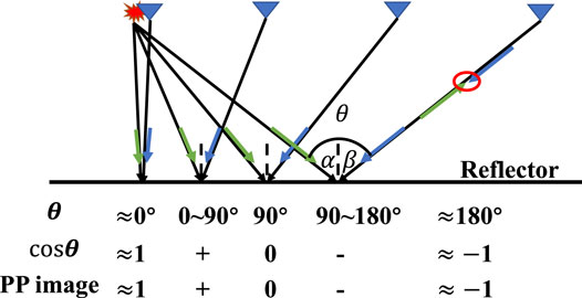
FIGURE 1. Sign distributions of PP images via the opening angles. The green arrows and blue arrows represent the P-wave incident vectors of the source wavefield and the reflected vectors of the receiver wavefield, respectively. Regardless of the incident and reflected vector’s modulus, the amplitude of PP images by the dot product scalar imaging condition implicitly depends on the scaling factor $\cos \theta$, where the opening angle $\theta$ is equal to the sum of the P-wave incident angle $\alpha$ and the reflected angle $\beta$. As for the unconverted reflection wave, the reflected angle $\beta$ is equal to the incident angle $\alpha$. The sign reversal of the factor$\cos \theta =\cos 2\alpha$ is observed when the incident angle $\alpha$approaches the critical angle $\mathrm{4}{\mathrm{5}}^{\circ }$, which indicates that polarity reversal occurs in the PP image. As marked by the red circle, the factor $\cos \theta$ reaches -1 while the incident angle is near $\mathrm{9}{\mathrm{0}}^{\circ }$, which exists in the propagation path of the backscattering wave. The backscattering artifacts with $\mathrm{18}{\mathrm{0}}^{\circ }$ or near $\mathrm{18}{\mathrm{0}}^{\circ }$ scattering angles (i.e., opening angles) also contaminate the PP image.

The Scalar Imaging Condition With the Laplace Filter

In acoustic RTM or scalar-based elastic RTM, the Laplace filter (Youn and Zhou, 2001) has been used to suppress the backscattering artifacts in the PP image. As for the PP image in vector-based elastic RTM, the scalar imaging condition with a Laplace filter can be expressed as follows:

$\begin{array}{l}{I}_{pp}^{lap}={\nabla }^2{I}_{PP}\\ ={\nabla }^2{\displaystyle \int \left({\mathbf{s}}^p\left(\mathbf{x},t\right)\cdot {\overline{\mathbf{r}}}^p\left(\mathbf{x},t\right)\right)dt}.\end{array}(6)$

Here, $I_{pp}^{lap}$ is the migrated PP image with a Laplace filter, ${\nabla }^2={\partial }_x^2+{\partial }_y^2+{\partial }_z^2$ is the Laplace filter operator, ${\partial }_x^2$, ${\partial }_y^2$, and ${\partial }_z^2$ are the second-order partial derivatives along the x-axis, y-axis, and z-axis direction, respectively. Since partial derivatives are independent of time integration, the PP image $I_{pp}^{lap}$ can also be disintegrated by Cartesian components’ cross-correlation imaging results. As for 2D vector-based wavefields, the PP image $I_{pp}^{lap}$ can be separated into four items:

$\begin{array}{l}{I}_{pp}^{lap}={\partial }_x^2{\displaystyle \int s_x^p{\overline{r}}_x^{p}dt}+{\partial }_x^2{\displaystyle \int s_z^p{\overline{r}}_z^{p}dt}+{\partial }_z^2{\displaystyle \int s_x^p{\overline{r}}_x^{p}dt}+{\partial }_z^2{\displaystyle \int s_z^p{\overline{r}}_z^{p}dt}\\ ={\partial }_x^2{I}_{ppxx}+{\partial }_x^2{I}_{ppzz}+{\partial }_z^2{I}_{ppxx}+{\partial }_z^2{I}_{ppzz}.\end{array}(7)$

Here, ${\partial }_x^2{I}_{ppxx}$ and ${\partial }_z^2{I}_{ppxx}$ are second-order derivatives of x-axis Cartesian component cross-correlation imaging result along the x-axis direction and z-axis direction, respectively; ${\partial }_x^2{I}_{ppzz}$ and ${\partial }_z^2{I}_{ppzz}$ are second-order partial derivatives of z-axis Cartesian component cross-correlation imaging result along the x-axis direction and z-axis direction, respectively. Thereinto, ${\partial }_x^2{I}_{ppxx}$ and ${\partial }_z^2{I}_{ppzz}$ are parallel-oriented partial derivatives of Cartesian component cross-correlation imaging result. Meanwhile, ${\partial }_z^2{I}_{ppxx}$ and ${\partial }_x^2{I}_{ppzz}$ are normal-oriented partial derivatives of Cartesian component cross-correlation imaging result. The fault model (shown in Figure 2) has been introduced for reverse time migration to highlight the interaction characteristics of these decoupled migrated results on the flat and inclined interface. Figures 3A–D are the decoupled migrated results of ${\partial }_x^2{I}_{ppxx}$, ${\partial }_x^2{I}_{ppzz}$, ${\partial }_z^2{I}_{ppxx}$, and ${\partial }_z^2{I}_{ppzz}$, respectively.

FIGURE 2

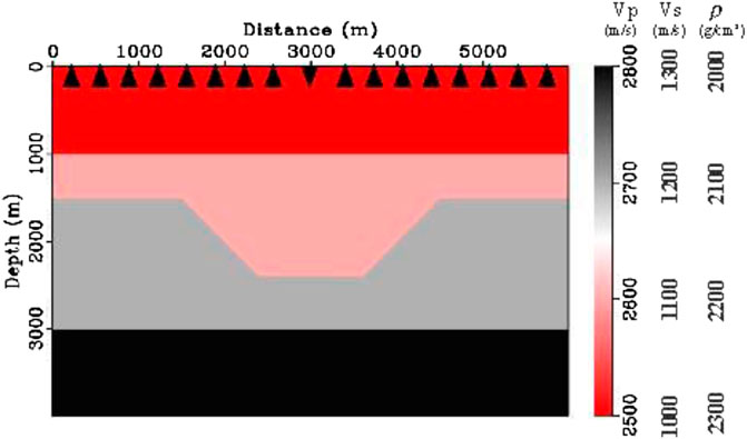
FIGURE 2. The P-wave velocity, S-wave velocity, and density of a fault model. The model contains 600 points of $dx=10m$in the x-axis and 400 points of $dz=10m$in the z-axis. The inverted triangle marks the location of the explosive source with a Ricker wavelet of 30 Hz, and triangle represents receivers with 20 m interval.

FIGURE 3

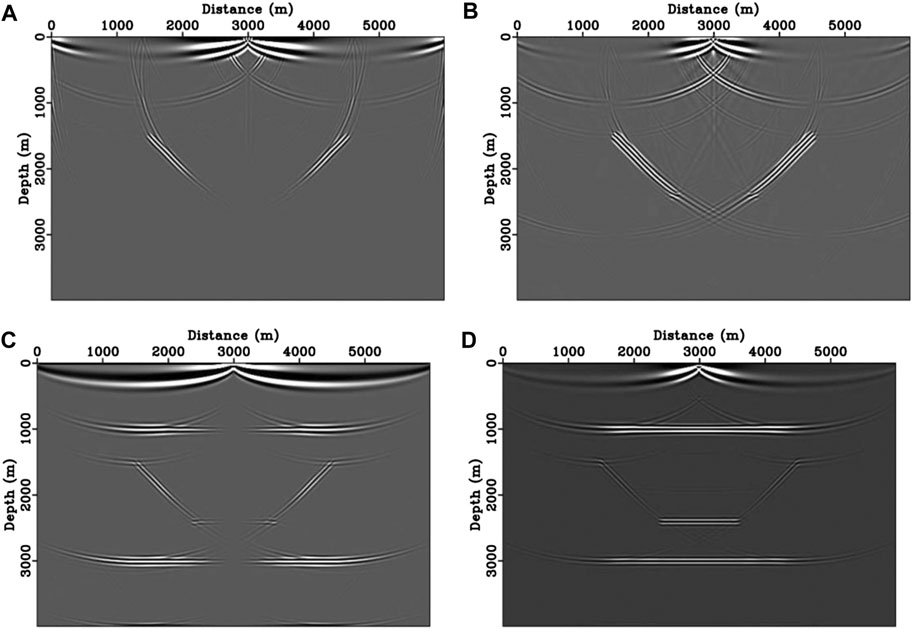
FIGURE 3. The decoupled migrated images of ${\partial }_x^2{I}_{ppxx}$(A), ${\partial }_x^2{I}_{ppzz}$(B), ${\partial }_z^2{I}_{ppxx}$(C), and ${\partial }_z^2{I}_{ppzz}$(D). The sum of decoupled migrated images ${\partial }_x^2{I}_{ppxx}$, ${\partial }_x^2{I}_{ppzz}$, ${\partial }_z^2{I}_{ppxx}$, and ${\partial }_z^2{I}_{ppzz}$ is equal to the scalar imaging condition with a Laplace filter $I_{pp}^{lap}$. Otherwise, the sum of decoupled migrated images ${\partial }_x^2{I}_{ppxx}$ and ${\partial }_z^2{I}_{ppzz}$ is equal to the scalar imaging condition with a pseudo-Laplace filter $I_{pp}^{pse-lap}$.

Backscattering noise has been suppressed in all decoupled images. Moreover, these decoupled images have different migration capabilities. On the one hand, the decoupled items ${\partial }_x^2{I}_{ppxx}$ (shown in Figure 3A) and ${\partial }_x^2{I}_{ppzz}$ (shown in Figure 3B) related to second-order partial derivative associated with x-axis direction show similar migrated images sensitive to inclined structures. Compared with the ideal parallel-oriented result ${\partial }_x^2{I}_{ppxx}$, the decoupled normal-oriented item ${\partial }_x^2{I}_{ppzz}$ would encounter severe crosstalks, causing destructive interference in the final stacked image. On the other hand, the decoupled items ${\partial }_z^2{I}_{ppxx}$ (Figure 3C) and ${\partial }_z^2{I}_{ppzz}$ (Figure 3D) related to second -order partial derivatives along the z-axis direction migrate good images in flat-layer structures. Compared with the ideal parallel-oriented migrated result ${\partial }_z^2{I}_{ppzz}$, the decoupled normal-oriented item ${\partial }_z^2{I}_{ppxx}$ fails to image near-zero offset, contrary to the final PP wave image. Furthermore, the phase of ${\partial }_z^2{I}_{ppxx}$ is opposite to ${\partial }_z^2{I}_{ppzz}$. The opposite phase between ${\partial }_z^2{I}_{ppzz}$ and ${\partial }_z^2{I}_{ppxx}$ will result in the Laplace filter’s disability in correcting the polarity reversal problem in the PP image. The scalar imaging condition with the Laplace filter successfully suppresses backscattering but fails to correct the polarity reversal.

The Scalar Imaging Condition With the Pseudo-Laplace Filter

Since normal-oriented partial derivative related items of the Laplace filter are greatly affected by crosstalk noise, the horizontal derivative related decoupled items have been selected to migrate the PP image. Analogous to the scalar imaging condition with the Laplace filter, we propose the scalar imaging condition with the pseudo-Laplace filter. To characterize the scalar imaging condition with a pseudo-Laplace filter mathematically, we first define the pseudo-Laplace operator ${\tilde{\nabla }}^2$ as follows:

${\tilde{\nabla }}^2=\left({\partial }_x^2,{\partial }_y^2,{\partial }_z^2\right)(8)$

and the PP wave’s Hadamard product image ${\mathbf{I}}_{PP}$ as follows:

${\mathbf{I}}_{PP}={\displaystyle \int {\mathbf{s}}^p\circ {\overline{\mathbf{r}}}^{p}dt}=\left(I_{ppxx},I_{ppyy},I_{ppzz}\right),(9)$

where $\circ$ is the Hadamard operator (see also Appendix A). The pseudo-Laplace operator ${\tilde{\nabla }}^2$ comprises three array components, which are second-order partial derivatives along the x-, y- and z-axis, respectively. Their summation is just the Laplace operator. Meanwhile, the PP wave Hadamard product images ${\mathbf{I}}_{PP}$ are composed of three array components: cross-correlation imaging results of the x-axis, y-axis, and z-axis Cartesian components. The summation of array components is just a PP wave scalar product image $I_{pp}$. There is some specific connection between the pseudo-Laplace operator ${\tilde{\nabla }}^2$ and the Laplace operator ${\tilde{\nabla }}^2$ and between the PP wave Hadamard product image ${\mathbf{I}}_{PP}$ and the PP wave scalar product image $I_{pp}$. Unlike the scalar Laplace operator ${\nabla }^2$ and PP wave scalar product image $I_{pp}$, the pseudo-Laplace operator ${\tilde{\nabla }}^2$ and PP wave Hadamard product image ${\mathbf{I}}_{PP}$ are both vectors.

Combining the pseudo-Laplace operator with the PP wave Hadamard product image vector, we propose a scalar imaging condition with a pseudo-Laplace filter for vector-based wavefields as follows:

$\begin{array}{l}{I}_{pp}^{pse-lap}={\tilde{\nabla }}^2\cdot {\mathbf{I}}_{PP}\\ ={\tilde{\nabla }}^2\cdot \left({\displaystyle \int {\mathbf{s}}^p\circ {\overline{\mathbf{r}}}^{p}dt}\right).\end{array}(10)$

Here, $I_{pp}^{pse-lap}$ is the PP image by the scalar imaging condition with a pseudo-Laplace filter. As for 2D vector-based wavefield, the scalar imaging condition with a pseudo-Laplace filter for the PP wave should be simplified, and components related to y-axis should be neglected:

$\begin{array}{l}{I}_{pp}^{pse-lap}={\partial }_x^2{\displaystyle \int s_x^p{\overline{r}}_x^{p}dt}+{\partial }_z^2{\displaystyle \int s_z^p{\overline{r}}_z^{p}dt}\\ ={\partial }_x^2{I}_{ppxx}+{\partial }_z^2{I}_{ppzz}.\end{array}(11)$

The scalar imaging conditions with a Laplace filter (Eq. 4) and a pseudo-Laplace filter (Eq. 8) depend on second-order partial derivatives of Cartesian components cross-correlation results. Different from the Laplace filter composed of parallel-oriented and normal-oriented items, only the parallel-oriented items are selected to form the pseudo-Laplace filter. As shown in Figure 4, we migrate the PP images of the fault model by the scalar imaging condition with the Laplace filter and with the pseudo-Laplace filter. Figure 4A is the migrated PP scalar image with a Laplace filter, the sum of Figures 3A–D. Similarly, the sum of Figures 3A,D is just one scalar migrated PP image with a pseudo-Laplace filter, as shown in Figure 4B. Compared with the PP image with a Laplace filter (Figure 4A), backscattering noise suppression (marked by red arrows) and polarity reversal correction (marked by red circles) have been shown in the PP image with a pseudo-Laplace filter (Figure 4B).

FIGURE 4

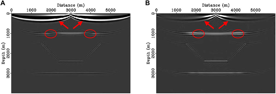
FIGURE 4. PP images by the scalar imaging condition with a Laplace filter (A) and with a pseudo-Laplace filter (B). Compared with the PP image with a Laplace filter (Panel A), backscattering noise suppression (marked by red arrows) and polarity reversal correction (marked by red circles) have been shown in the PP image with a pseudo-Laplace filter (Panel B).

For the application in elastic RTM, we should migrate three Cartesian component’s images (or two images in a 2D case) by time integration and then sum second-order derivatives of three images together. Compared with the scalar imaging condition, additional storage of three Cartesian component’s images and computation of second-order derivative operation are introduced in scalar imaging conditions with a pseudo-Laplace filter. Compared with the storage and computation costs consumed by the wavefield extrapolation of elastic RTM, the additional calculation introduced by the proposed filter can be ignored to a certain degree. Thus, the scalar imaging condition with a pseudo-Laplace filter is easy to perform and does not require additional processing or storage, which is essential for elastic RTM.

Backscattering Attenuation and Polarity Correction

Based on the above-tested fault model, the suppression of backscattering and correction of polarity reversal have been shown in the PP scalar image with the proposed pseudo-Laplace filter. The section will theoretically illustrate how the pseudo-Laplace filter suppresses backscattering noise and correct polarity reversal in PP images with the assumption of a plane wave.

For the vector-based elastic wavefields, the source-side particle velocity vector ${\mathbf{s}}^p$ and receiver-side particle velocity vector ${\mathbf{r}}^p$ are related to the polarization and propagation of the P wave. Decomposing the particle velocity wavefield of pure P wave in plane waves, we obtain the following:

${\mathbf{s}}^p=\left|{\mathbf{s}}^p\right|{\mathbf{p}}^s{e}^{ik\left({\mathbf{n}}^s\cdot \mathbf{x}-v_{p}t\right)},(\mathrm{12A})$

and

${\overline{\mathbf{r}}}^p=\left|{\mathbf{r}}^p\right|R_{pp}{\mathbf{p}}^r{e}^{ik\left(v_{p}t-{\mathbf{n}}^r\cdot \mathbf{x}\right)}.(\mathrm{12B})$

Here, $\left|{\mathbf{s}}^p\right|$and $\left|{\mathbf{r}}^p\right|=\left|{\mathbf{s}}^p\right|R_{pp}$ are the modulus of the incident and reflected wave, respectively. $\mathbf{p}$ and $\mathbf{n}$ are polarization unit vector and propagation unit vector, respectively. Superscripts s and r represent incident wave and reflected wave. $v_p$, $k=\omega /v_p$, and $\omega$ are P wave’s propagated velocity, wavenumber and angular frequency, respectively. Assuming that vectors $\mathbf{n}$ and $\mathbf{p}$ vary slowly in the space-time domain, their temporal and spatial derivatives are small enough to be ignored.

Substituting the plane wave definitions (Eq. 12) into Eqs 4, 7, 11, we obtain an expression with the assumption of the plane wave as follows:

$I_{pp}={\displaystyle \int \left|{\mathbf{s}}^p\right|\left|{\mathbf{r}}^p\right|R_{pp}\left({\mathbf{p}}^s\cdot {\mathbf{p}}^r\right)e^{ik\left({\mathbf{n}}^s-{\mathbf{n}}^r\right)\cdot \mathbf{x}}dt},(\mathrm{13A})$

$I_{pp}^{lap}=-{\displaystyle \int \left|{\mathbf{s}}^p\right|\left|{\mathbf{r}}^p\right|R_{pp}{\omega }^2\left\{\left[{\left(n_x^s-n_x^r\right)}^2+{\left(n_z^s-n_z^r\right)}^2\right]\left(p_x^s{p}_x^r+p_z^s{p}_z^r\right)\right\}{e}^{ik\left({\mathbf{n}}^s-{\mathbf{n}}^r\right)\cdot \mathbf{x}}dt},(\mathrm{13B})$

and

$I_{pp}^{pse-lap}=-{\displaystyle \int \left|{\mathbf{s}}^p\right|\left|{\mathbf{r}}^p\right|R_{pp}{\omega }^2\left[{\left(n_x^s-n_x^r\right)}^2{p}_x^s{p}_x^r+{\left(n_z^s-n_z^r\right)}^2{p}_z^s{p}_z^r\right]e^{ik\left({\mathbf{n}}^s-{\mathbf{n}}^r\right)\cdot \mathbf{x}}dt}.(\mathrm{13C})$

In the 2D case of incident pure P wave, the reflected P wave without wave conversion would be obtained in an observation coordinate system along the horizontal surface and vertical depth. As shown in Figure 5A, the geological structure information of the reflector has been introduced in the descriptions of particle velocity vectors in the observation coordinate system. A local coordinate system (as shown in Figure 5B) is constructed along with tangential and vertical directions of the reflector to simplify the representation of vectors in the source and receiver wavefield. As for pure P wave, the polarization vector ${\mathbf{p}}^s$ is parallel to the propagation vector ${\mathbf{n}}^s$ with the same positive direction. In the local coordinate system, the polarization vector ${\mathbf{p}}^s$ and propagation vector ${\mathbf{n}}^s$ of incident vector ${\mathbf{s}}^p$ in source wavefield should be described by the incident angle $\alpha$ as follows:

${\mathbf{p}}^s=\sin \alpha \overrightarrow{i}+\cos \alpha \overrightarrow{k},(\mathrm{14A})$

and

${\mathbf{n}}^s=\sin \alpha \overrightarrow{i}+\cos \alpha \overrightarrow{k}.(\mathrm{14B})$

Unlike source wavefield, the pure P wave in receiver wavefield should be described by conjugation of a reflected vector ${\overline{\mathbf{r}}}^p$. Its propagation direction is the opposite to that of the reflected wave, and polarization direction is the same as the reflected wave. The polarization vector ${\mathbf{p}}^s$ is parallel to the propagation vector ${\mathbf{n}}^s$ with the same positive direction for reflected pure P wave ${\mathbf{r}}^p$. When it comes to reflected pure P wave, the polarization vector ${\mathbf{p}}^r$ and propagation vector ${\mathbf{n}}^r$ should be described in the local coordinate system by the reflected angle $\alpha$ as follows:

${\mathbf{p}}^r=-\sin \alpha \overrightarrow{i}+\cos \alpha \overrightarrow{k},(\mathrm{15A})$

and

${\mathbf{n}}^r=\sin \alpha \overrightarrow{i}-\cos \alpha \overrightarrow{k}.(\mathrm{15B})$

According to the descriptions of incident vector (Eq. 14) and conjugation of reflected vector (Eq. 15), we can rewrite the scalar imaging condition, the scalar imaging condition with a Laplace filter, and the scalar imaging condition with a pseudo-Laplace filter in the local Cartesian coordinate system as follows:

$I_{pp}={\displaystyle \int \left|{\mathbf{s}}^p\right|\left|{\mathbf{r}}^p\right|R_{pp}\cos \theta e^{ik\left({\mathbf{n}}^s-{\mathbf{n}}^r\right)\cdot \mathbf{x}}dt},(\mathrm{16A})$

$I_{pp}^{lap}=-{\displaystyle \int \left|{\mathbf{s}}^p\right|\left|{\mathbf{r}}^p\right|R_{pp}{\omega }^{2}2\cos \theta \left(\cos \theta +1\right)e^{ik\left({\mathbf{n}}^s-{\mathbf{n}}^r\right)\cdot \mathbf{x}}dt},(\mathrm{16B})$

FIGURE 5

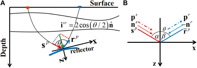
FIGURE 5. The incident vector and reflected vector of pure P wave in observation coordinate system (A) and local coordinate system (B). The coordinate observation system is constructed along the horizontal surface and vertical depth. The illumination vector ${\mathbf{i}}^{sr}$, used to describe the relationship between the incident wave and reflected wave, is related to the vertical directions of the reflector and opening angle. To simplify their representation, the local coordinate system is constructed along with tangential and vertical directions of the reflector. In a local coordinate system, the incident vector and reflected vector can be described by the incident angle $\alpha$ or opening angle $\theta$.

and

$I_{pp}^{pse-lap}=-{\displaystyle \int \left|{\mathbf{s}}^p\right|\left|{\mathbf{r}}^p\right|R_{pp}{\omega }^2{\left(\cos \theta +1\right)}^2{e}^{ik\left({\mathbf{n}}^s-{\mathbf{n}}^r\right)\cdot \mathbf{x}}dt}.(\mathrm{16C})$

Here, $\theta =2\alpha$ is the opening angle. The above-mentioned imaging algorithms need to be separated into terms related to amplitude and phase. As for the phase-related item, they agree with each other by the form of $e^{ik\left({\mathbf{n}}^s-{\mathbf{n}}^r\right)\cdot \mathbf{x}}$. The phase-related item is dependent on the illumination vector ${\mathbf{i}}^{sr}={\mathbf{n}}^s-{\mathbf{n}}^r$, defined by Lecomte (2008). The illumination vector ${\mathbf{i}}^{sr}$ satisfies the following relationship ${\mathbf{i}}^{sr}={\mathbf{n}}^s-{\mathbf{n}}^r=2\cos \left(\theta /2\right)\widehat{\mathbf{n}}$, where $\widehat{n}$ is a unit normal vector at each reflector. In a local coordinate system, a unit normal vector can be described as $\widehat{\mathbf{n}}=\left(\mathrm{0,1}\right)$ regardless of the inclination of a reflector. Phase-related items are dependent on the opening angle $\theta$. In particular, ${\mathbf{i}}^{sr}=0$ while $\theta =180°$. It indicates that ${\mathbf{i}}^{sr}$ will be zero at the reflectors when the incident wave and reflected wave are with the same propagating path.

Otherwise, the amplitude-related items in $I_{pp}$, $I_{pp}^{lap}$, and $I_{pp}^{pse-lap}$ imaging algorithms are different from each other. Factor $\left|{\mathbf{s}}^p\right|\left|{\mathbf{r}}^p\right|R_{pp}$, coexisting in The above-mentioned imaging conditions, is useful for seismic inversion interpretation. Once the Laplace filter and pseudo-Laplace filter are introduced, the scalar imaging algorithms are influenced by angular frequency ${\omega }^2$. The introduction of ${\omega }^2$ weakens the amplitude of low-frequency data and enhances the amplitude of high-frequency data, changing the spectrum of images and damaging effective low-frequency information. To maintain the spectrum of images and recover their effective low-frequency information, reasonable time integration is needed (Liu et al., 2010). Furthermore, the above-mentioned imaging algorithms are dependent on different weighting factors:

$w_{pp}=\cos \theta ,(\mathrm{17A})$

$w_{pp}^{lap}=-2\cos \theta \left(\cos \theta +1\right),(\mathrm{17B})$

and

$w_{pp}^{pse-lap}=-{\left(\cos \theta +1\right)}^2.(\mathrm{17C})$

Here, $w_{pp}$,$w_{pp}^{lap}$, and $w_{pp}^{pse-lap}$ are the introduced weighting factor of the scalar imaging condition, the scalar imaging condition with a Laplace filter, and the scalar imaging condition with a pseudo-Laplace filter, respectively. From Eq. 17, we can see that weighting factors vary with the opening angle $\theta$.

The variation of the weighting factor for the opening angle $\theta$ is shown in Figure 6. For visual display, the amplitude is normalized by the corresponding max value. When the opening angle $\theta$ increases from ${\mathrm{0}}^{\circ }$ to $\mathrm{18}{\mathrm{0}}^{\circ }$, the weighting factor $w_{pp}$ (represented by the blue curve) in the scalar imaging condition ranges from 1 through 0 to −1. The polarity of the image is reversed while the sign of weight factor changes from positive to negative near $\mathrm{9}{\mathrm{0}}^{\circ }$, and the backscattering noise is generated by dot product cross-correlation of two wavefields with an opening angle of $\mathrm{18}{\mathrm{0}}^{\circ }$ or close to $\mathrm{18}{\mathrm{0}}^{\circ }$. By introducing the Laplace filter, the weighting factor $w_{pp}^{lap}$ (represented by the red curve) will be 0 near $\mathrm{18}{\mathrm{0}}^{\circ }$, which indicates that backscattering noise has been suppressed. However, the sign of the weighting factor $w_{pp}^{lap}$ still changes from positive to negative around $\mathrm{9}{\mathrm{0}}^{\circ }$. In other words, the Laplace filter fails to correct the polarity reversal in PP images by scalar imaging conditions. Furthermore, the pseudo-Laplace filter has been introduced in scalar imaging conditions, and its weighting factor $w_{pp}^{pse-lap}$ (represented by the yellow curve) is in the range of 1–0. Similar to the Laplace filter, for backscattering waves with $\mathrm{18}{\mathrm{0}}^{\circ }$ or near $\mathrm{18}{\mathrm{0}}^{\circ }$ opening angles, the weighting factor $w_{pp}^{pse-lap}$ is zero. Unlike the Laplace filter, the weighting factor $w_{pp}^{pse-lap}$ only ranges from 1 to 0, and its sign is always positive. Therefore, the weighting factor can suppress backscattering noise and correct the reversed polarity. As for the PP image by the scalar imaging condition with a pseudo-Laplace filter, the backscattering noise has been suppressed and polarity reversal has been corrected.

FIGURE 6

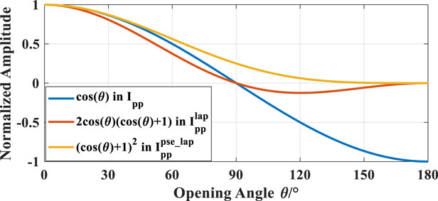
FIGURE 6. The variation of a weighting factor in the scalar imaging condition, the scalar imaging condition with a Laplace filter and with a pseudo-Laplace filter. Note that the blue curve of the weighting factor $\cos \theta$ will cross through the axis whose amplitude is zero and reach -1 while the opening angle is $\mathrm{18}{\mathrm{0}}^{\circ }$. The red curve of the weighting factor $2\cos \theta \left(\cos \theta +1\right)$ goes through the axis whose amplitude is zero and reaches 0 while the opening angle is $\mathrm{18}{\mathrm{0}}^{\circ }$. The yellow curve of the weighting factor ${\left(\cos \theta +1\right)}^2$ range 1–0 without change of positive and negative sign.

Numerical Examples

This section presents a two-layer flat model and a four-layer inclined model to demonstrate the challenges of backscattering noise and polarity reversal in PP images caused by scalar imaging conditions. Moreover, it shows how to suppress them by the pseudo-Laplace filter. Then, using numerical values, we investigate the amplitude variation versus the opening angle to demonstrate the consistency of the pseudo-Laplace filter. The Marmousi 2 model (Martin et al., 2006) is then used to demonstrate the effectiveness and advantages of the pseudo-Laplace filter in the suppression of backscattering artifacts and correction of polarity reversal.

When it comes to vector-based elastic RTM, the decoupled elastic wave equation (Xiao and Leaney, 2010; Du et al., 2017) generates source and receiver wavefield of decoupled P wave. Furthermore, the source normalization by decoupled P-wave source wavefield should be introduced to balance the energy between the shallow and deep layers.

The Two-Layer Flat Model

The two-layer flat model shown in Figure 7 is $10\times 2km$. At a depth of 1 km, there is one flat interface. The first and second layer’s P-wave velocities would be 2400 m/s and 2700 m/s, respectively. The S-wave velocity is consistent with the relationship $v_s=v_p/1.73$, and density is set to 1.0 g/cm³. It contains 1000 points in the horizontal direction and 200 points in the vertical direction, with a space interval of 10 m. Figure 8 shows a synthetic seismic record generated using double receiving observation geometry, with a shot located at a depth of 10 m. At a depth of 10 m, there are 500 receivers with a 20 m receiver interval. As a result, the maximum offset is up to 5 km. The synthetic seismic data are generated using an explosive source of Ricker wavelet with a peak frequency of 20 Hz. The time interval is 0.8 ms, and the total record time is 2.4 s.

FIGURE 7

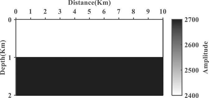
FIGURE 7. The P-wave velocity of the two-layer flat model, whose S-wave velocity and density are satisfied with $v_s=v_p/1.73$ and $\rho =2300g/c{m}^2$, respectively.

FIGURE 8

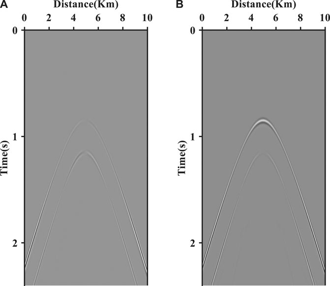
FIGURE 8. The synthetic multicomponent seismic record without direct wave: (A) x-component and (B) z-component.

The migrated PP images by scalar imaging conditions, scalar imaging conditions with a Laplace filter, and scalar imaging conditions with a pseudo-Laplace filter are shown in Figure 9. It is evident that backscattering artifacts (marked by the red arrow) influence the PP image by the scalar imaging condition (shown in Figure 9A) and have been attenuated effectively in the PP image with the application of a Laplace filter (shown in Figure 9B) and with a pseudo-Laplace filter (shown in Figure 9C). Apart from backscattering noise, the other noise, such as polarity reversal, also occurs at the interface. As for the interface of 1 km depth, the maximum incident angle reaches $\mathrm{68}\mathrm{.}{\mathrm{2}}^{\circ }$, over critical angle $\arcsin \left(v_{p1}/v_{p2}\right)=62.73°$ and polarity reversed angle $\mathrm{4}{\mathrm{5}}^{\circ }$. Thus, all three migrated PP images are similar and encounter phase-distorted inhomogeneous waves, such as refracted waves (marked by blue arrows) around 1.9 km distance. Besides, only PP images without or with the Laplace filter suffer from the polarity reversal around 1 km distance (marked by red circles), which would have been corrected in the PP image with a pseudo-Laplace filter. Therefore, the phase axis of the PP image with the pseudo-Laplace filter is more continuous than the PP image with the Laplace filter.

FIGURE 9

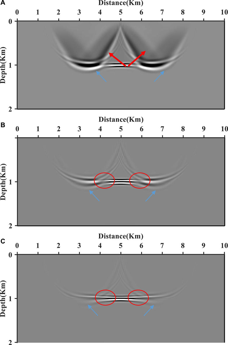
FIGURE 9. PP migrated images of the two-layer flat model by the scalar imaging condition (A), the scalar imaging condition with a Laplace filter (B), and the scalar imaging condition with a pseudo-Laplace filter (C). The backscattering noise (marked by the red arrow) has been effectively suppressed in PP images by scalar imaging conditions with a Laplace filter and a pseudo-Laplace filter. Furthermore, the polarity reversal (marked by the red circle) has been corrected in the PP image by the scalar imaging condition with a pseudo-Laplace filter.

Additionally, we measure the amplitudes of these images at the interface at a depth of 1 km and convert the offset variable to the opening angle variable using geological and elastic parameters. Then, we compare these amplitudes (blue curves) from Figure 9 with the theoretical reflection coefficient $R_{pp}$ (yellow curves) and the corresponding weighting factor (red curves), respectively. The analytical solution $R_{pp}$ (yellow curves) is calculated by solving the Zoeppritz equation with the elastic parameters of the two-layer layer model. The opening angle ranges from 0 to 120° to avoid phase distortion when the incidence angle is greater than the critical angle of 62.73°. The extracted amplitudes (blue curves) match well with the weighting theoretical reflection coefficient (red curves) up to approximately 80°, verifying the correctness of the theoretical analysis.

What is more, the extracted amplitudes have higher values than the corresponding weighting theoretical reflection coefficient at large angles of incidence and then decline to zero due to the limited acquisition space. Both Laplace and pseudo-Laplace filters would fail to maintain the amplitude of images at large incidence. Figure 10A shows the extracted amplitudes from Figure 9A and weighting theoretical reflection coefficient $R_{pp}\cos \theta$; Figure 10B shows the extracted amplitudes from Figure 9B and weighting theoretical reflection coefficient $R_{pp}\cos \theta \left(\cos \theta +1\right)$. They both change their signs at approximately 90° angle of incidence. However, Figure 10C shows the extracted amplitudes from Figure 9C and weighting theoretical reflection coefficient $R_{pp}{\left(\cos \theta +1\right)}^2$, and its sign remains unchanged at any opening angle. Therefore, the consistency of the pseudo-Laplace filter has been demonstrated by the analysis of amplitude variation versus the opening angle, which indicated that polarity reversal had been corrected.

FIGURE 10

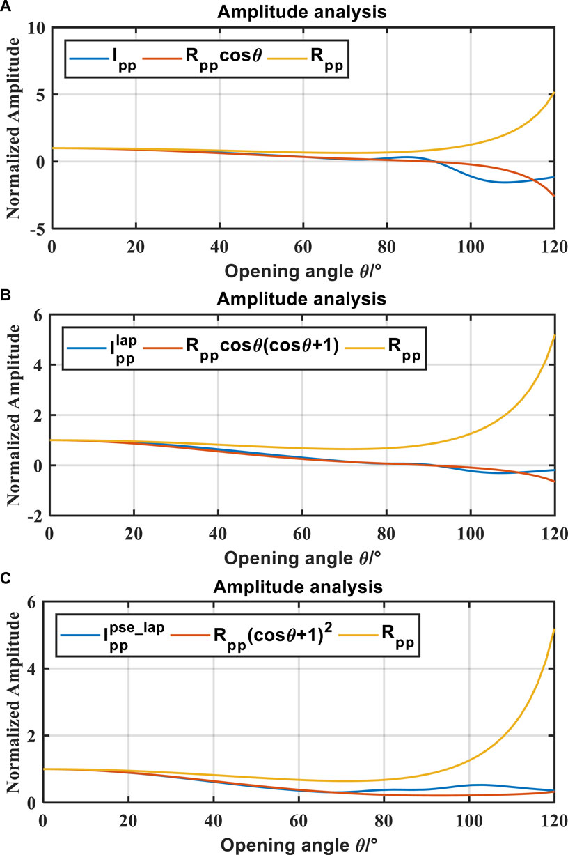
FIGURE 10. The comparison between the analytical reflection coefficient $R_{pp}$ (yellow curves), the weighting theoretical reflection coefficient (red curves) and normalized amplitudes (blue curves) extracted from PP images by the scalar imaging condition (A), the scalar imaging condition with a Laplace filter (B), and the scalar imaging condition with a pseudo-Laplace filter (C) in Figure 9. The reflection coefficient (yellow curves) is solved by the Zoeppritz equation with the elastic parameters of the two-layer layer model, and the normalized amplitudes in PP images have been converted to variation with the opening angle.

The Four-Layer Inclined Model

The four-layer inclined model, as shown in Figure 11, is $10\times 4km$. There are three inclined interfaces with a $\mathrm{1}{\mathrm{0}}^{\circ }$ dip angle at 1.5, 2.5, and 3.5 km depth, respectively. The P-wave velocity of the first layer, second layer, third layer, and fourth layer would be 2500 m/s, 2600 m/s, 2700 m/s, and 2800 m/s, respectively. The S-wave velocity satisfies the relationship $v_s=v_p/1.73$, and density is set to constant 1 g/cm³. It contains 1000 points and 400 points in the horizontal and vertical directions with a space interval of 10 m. Synthetic data are generated with double receiving observation geometry, where the shot is located at a depth of 10 m and a distance of 7 km. There are 500 receivers with a receiver interval of 20 m at a depth of 10 m. Therefore, the maximum offset is 7 km. The explosive source of the Ricker wavelet with 30 Hz peak frequency is set to generate the synthetic seismic data. The time interval is 1.0 ms, and the total record time is 3 s.

FIGURE 11

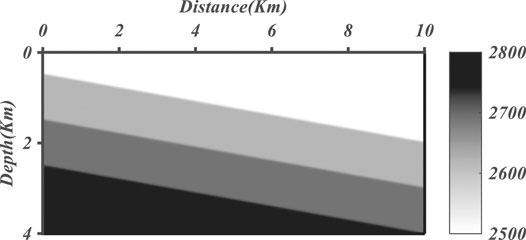
FIGURE 11. The P-wave velocity of the four-layer inclined model, whose S-wave velocity and density are satisfied with $v_s=v_p/1.73$ and $\rho =2300g/c{m}^2$, respectively.

The migrated PP images by scalar imaging conditions with a Laplace filter and scalar imaging conditions with a pseudo-Laplace filter are shown in Figure 12. It is evident that backscattering artifacts (marked by the red arrow) influence the PP image by scalar imaging conditions (shown in Figure 12A) and have been attenuated effectively in the PP image with the application of a Laplace filter (shown in Figure 12B) and with a pseudo-Laplace filter (shown in Figure 12C). Apart from backscattering noise, the other noise, such as polarity reversal, also occurs at images along with the interfaces. As for the first interface, the maximum incident angle reaches $\mathrm{7}{\mathrm{5}}^{\circ }$, which is over critical angle $\arcsin \left(v_{p1}/v_{p2}\right)=74.05°$, and polarity reversed angle $\mathrm{4}{\mathrm{5}}^{\circ }$ at the maximum offset of 7 km. Therefore, the polarity reversal around 5 km (marked by a red circle) and phase-distorted homogeneous wave such as refracted wave (marked by the blue arrow) would be introduced in PP images without or with a Laplace filter. As for the second interface, the maximum incident angle of $\mathrm{5}{\mathrm{8}}^{\circ }$, equal to $\mathrm{11}{\mathrm{6}}^{\circ }$ opening angle, is less than the critical angle $\arcsin \left(v_{p2}/v_{p3}\right)=74.35°$ and bigger than the polarity reversed angle of $\mathrm{4}{\mathrm{5}}^{\circ }$. PP images without or with the Laplace filter of the second interface only encounter a polarity reversal problem around 4 km without phase aberration. As for the third interface, the maximum incident angle of $\mathrm{4}{\mathrm{3}}^{\circ }$ is near the polarity reversed angle of $\mathrm{4}{\mathrm{5}}^{\circ }$ and less than the critical angle $\arcsin \left(v_{p2}/v_{p3}\right)=74.64°$. The amplitude of the phase-reversed image is too little to influence the final stacked result. Furthermore, the polarity reversals at three interfaces have been corrected in the PP image with a pseudo-Laplace filter. Therefore, the phase axis of the PP image with a pseudo-Laplace filter is more continuous than the PP image with a Laplace filter.

FIGURE 12

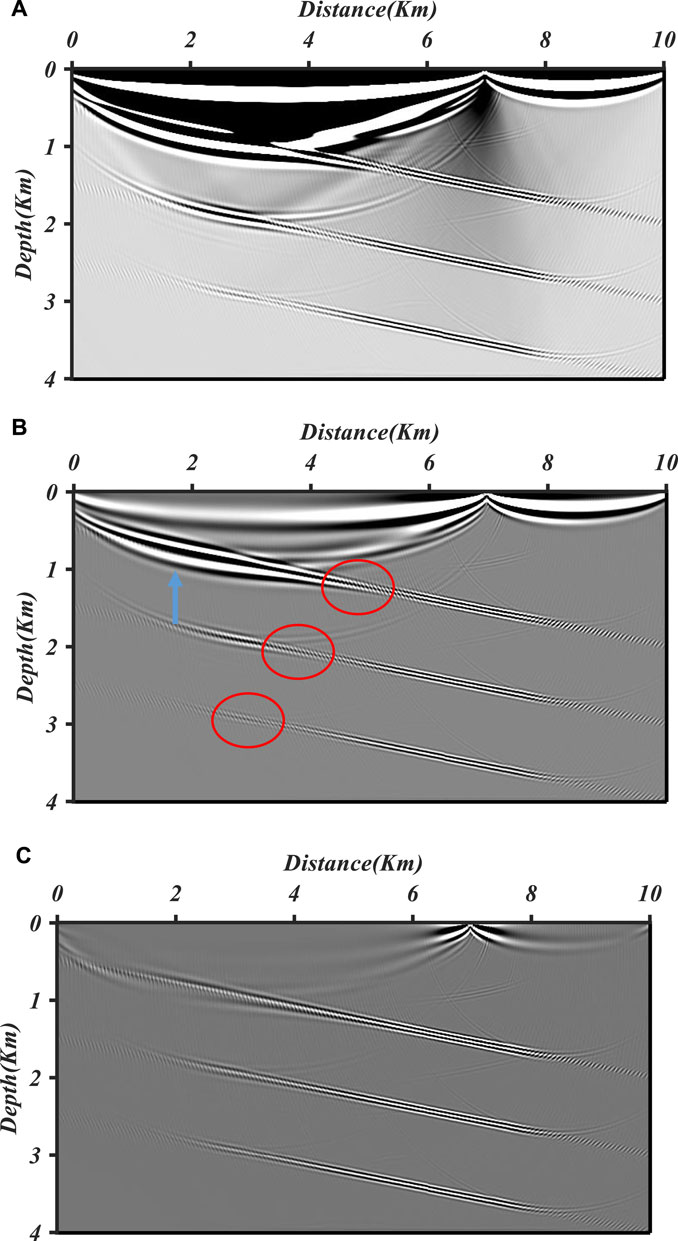
FIGURE 12. PP migrated images of the four-layer inclined model by the scalar imaging condition (A), the scalar imaging condition with a Laplace filter (B), and the scalar imaging condition with a pseudo-Laplace filter (C). The backscattering noise (marked by the red arrow) has been effectively suppressed in PP images by scalar imaging conditions with a Laplace filter and a pseudo-Laplace filter. Furthermore, the polarity reversal (marked by the red circle) has been corrected in the PP image by the scalar imaging condition with a pseudo-Laplace filter.

To analyze the amplitude variation versus opening angle, we pick up the max amplitude of these images along the second interface and convert the offset variable to the opening angle variable with a geological structure. Since the first interface is affected by the direct wave and heterogeneous wave such as refracted wave, the second interface has been utilized. Once the amplitude variation has been picked up, the smoothing and normalization are required to avoid interference of other factors such as phase. As shown in Figure 13, the variations of normalized amplitude in three images match the variations of normalized weighting with an opening angle ranging from 0 to near $\mathrm{11}{\mathrm{6}}^{\circ }$, the maximum opening angle of the geometry. Once the opening angle exceeds the maximum, normalized amplitudes would be zero. Around $\mathrm{9}{\mathrm{0}}^{\circ }$ opening angle, change the numerical symbols of amplitude that occurs in the PP image (represented by the blue curve) and the PP image with a Laplace filter (represented by the red curve). However, the yellow curve, representing the PP image with a pseudo-Laplace filter, has a consistent numerical symbol in amplitude. Therefore, the consistency of the pseudo-Laplace filter has been demonstrated by the analysis of amplitude variation versus the opening angle, which indicated that polarity reversal had been corrected.

FIGURE 13

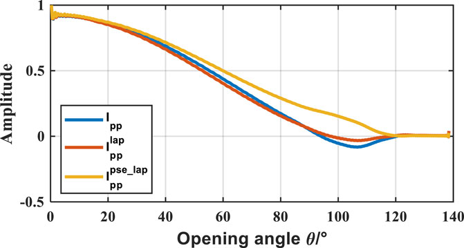
FIGURE 13. The variation of normalized amplitude in PP images with the opening angle. Numerically, amplitude symbols change with the P-wave incident angle reaching $\mathrm{4}{\mathrm{5}}^{\circ }$, and the offset is around 3500 m in both the PP image by the scalar imaging condition (blue curve) and the scalar imaging condition with a Laplace filter (red curve). In contrast, amplitude symbols are consistent in the PP image by the scalar imaging condition with a pseudo-Laplace filter (yellow curve).

Marmousi 2 Model

The Marmousi 2 model is used in this example to show how the pseudo-Laplace filter can effectively suppress backscattering noise, resolve polarity reversal, and generate a high-quality PP image in complex geological structures.

As shown in Figure 14, the modified Marmousi 2 model (Martin et al., 2006) contains 1325 points in the horizontal direction with 10 m sample interval and 934 points in the vertical direction with 5 m sample interval. Thus, the size of the Marmousi 2 model is $13.25\times 4.67km$. The P-wave velocity ranges from 1800 m/s to 4600 m/s, the S-wave velocity ranges from 1000 m/s to 2000 m/s, and density is the constant of 1 g/cm³. The full-receiving geometry, where 265 shots are excited with a 50 m shot interval at a depth of 10 m, and 1325 receivers are located with a 10 m receiver interval at the surface, is constructed to generate the seismic record. The source function is a Ricker wavelet with a peak frequency of 30 Hz. The recording time interval is 1.0 ms, and the recording length is 4.3 s.

FIGURE 14

FIGURE 14. The P-wave velocity of the elastic Marmousi 2 model (A) and the S-wave velocity of the elastic Marmousi 2 model (B) and the density is constant of 1 g/cm³.

Figure 15A is the migrated PP image by the scalar imaging condition with the Laplace filter, and Figure 15B is the migrated PP image by the scalar imaging condition with a pseudo-Laplace filter. The backscattering noise contamination has been suppressed successfully in these two images, while some backscattering noise still resides in the PP image with Laplace (marked by the red arrow). Furthermore, both of them have embodied the structural character of the model. Compared with the PP image with Laplace of Figure 15A, the overall appearance of Figure 15B is more apparent, including the shallow fault in detail. That is related to the weighting factor of the pseudo-Laplace filter is stronger than that of the Laplace filter. Furthermore, the events in the shallow layer of Figure 15B are more continuous than those of Figure 15A.

FIGURE 15

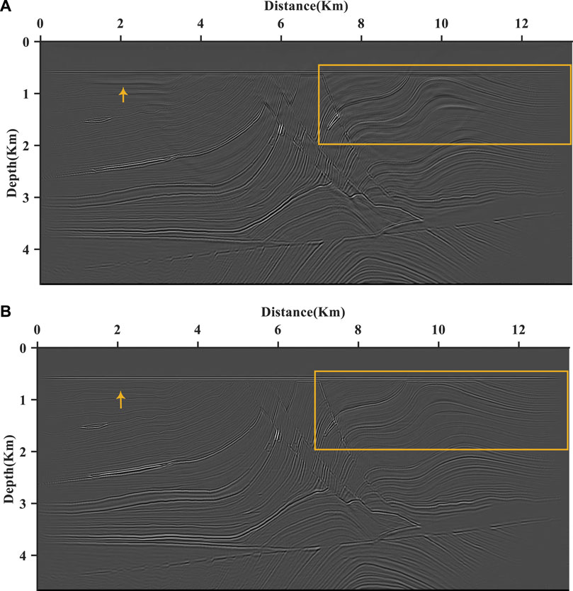
FIGURE 15. The PP images of the Marmousi 2 model by the scalar imaging condition with the Laplace filter (A) and with the pseudo-Laplace filter (B). The two images embody the structural characteristics of the model. The overall appearance of Panel B is more apparent and events in the shallow layer are more continuous than those in Panel A. Furthermore, the backscattering noise of Panel A is more serious than that in Panel B.

We further extracted the traces from PP images with a Laplace filter (Figure 15A) and a pseudo-Laplace filter (Figure 15B) at a depth of 1.32 km. As shown in Figure 16, we compare the amplitude of trace extracted from Figure 15A (blue curve) and Figure 15B (red curve) with the theoretical reflection coefficient $R_{pp}$ (yellow curves). The Zoeppritz equation calculates the theoretical reflection coefficient $R_{pp}$ at normal incidence. The variation trends of traces are consistent with the theoretical reflection coefficient. Moreover, the amplitude of trace from $I_{pp}^{pse\_lap}$ (red curve) is generally slightly larger than that from $I_{pp}^{lap}$ (blue curve) because the weighting factor $2\cos \theta \left(\cos \theta +1\right)$ of PP images with a Laplace filter is stronger than the weighting factor ${\left(\cos \theta +1\right)}^2$ of PP images with the pseudo-Laplace filter at small incident angles. However, there is a big difference between amplitudes and theoretical value in the fault area at 5–6 km and 7–8 km. The inaccuracy is caused by a false reflected wave where diffraction wave and multiple waves exist. Moreover, at the cover of anticline where sub-cover oil and gas reservoirs develop with 10–11 km distance, the phase of stacked $I_{pp}^{lap}$ (blue curve) is opposite to that of stacked $I_{pp}^{pse\_lap}$ (red curve) and theoretical solution (yellow curve), as marked by a black rectangular box. The phase reversal originates from polarity reversal in the PP image with the Laplace filter and polarity correction in the PP image with the pseudo-Laplace filter at large incidence.

FIGURE 16

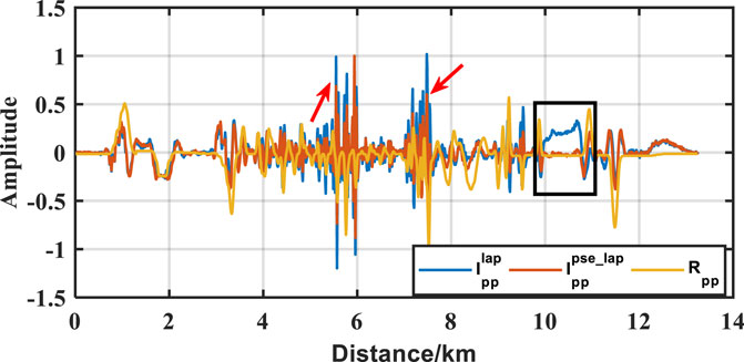
FIGURE 16. The comparison between normalized amplitudes of theoretical reflection coefficient $R_{pp}$ (yellow curves) calculated by Zoeppritz equation and traces extracted from Figure 15A (blue curve) and Figure 15B (red curve) at a depth of 1.32 km. The variation trends of traces are consistent with the theoretical reflection coefficient, and the amplitude of trace from $I_{pp}^{pse\_lap}$ (red curve) is generally slightly larger than that from $I_{pp}^{lap}$ (blue curve). However, the amplitude of trace from $I_{pp}^{pse\_lap}$ (red curve) is smaller than that from $I_{pp}^{lap}$ (blue curve) in the fault area (marked by the red arrow). Moreover, the phase of $I_{pp}^{lap}$ (blue curve) is opposite to that of $I_{pp}^{pse\_lap}$ (red curve) and theoretical solution (yellow curve) at the cover of anticline where sub-cover oil and gas reservoirs develop, marked by a black rectangular box.

To observe clearly, we intercept the part of the Marmousi 2 model with a distance from 7–13 km and a depth from 0.5 to 4 km. Figures 17A,B are the partial enlargements of the P-wave velocity of the elastic Marmousi 2 model and S-wave velocity of the elastic Marmousi 2 model amplified, respectively. Correspondingly, Figure 18A is a partial enlargement of the PP image of the Marmousi 2 model by the scalar imaging condition with a Laplace filter (Figure 15A), and Figure 18B is a partial enlargement of the PP image of the Marmousi 2 model by the scalar imaging condition with the pseudo-Laplace filter (Figure 15B). Even as the polarity reversal described by Figure 16, the phase of the stacked PP image with a Laplace filter is opposite to that of the stacked PP image with a pseudo-Laplace filter and is no longer continuous at the cover of the anticline. As marked by the blue curve, the phase of the event in Figure 18B is more persistent than in Figure 18A, especially at the cover of an anticline. Furthermore, there is an oil and gas reservoir at sub-cover with the variation of S-wave velocity in Figure 17B. The disturbance at sub-cover (marked by the red arrow) succeeds to be imaged in Figure 18A but fails to be imaged in Figure 18A. Overall, the scalar imaging condition with a pseudo-Laplace filter generates a high-quality PP image in complicated geological structures.

FIGURE 17

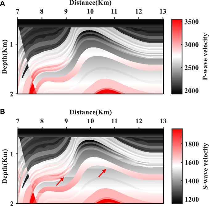
FIGURE 17. The partial enlargements of the P-wave velocity of the elastic Marmousi 2 model (A) and the S-wave velocity of the elastic Marmousi 2 model (B).

FIGURE 18

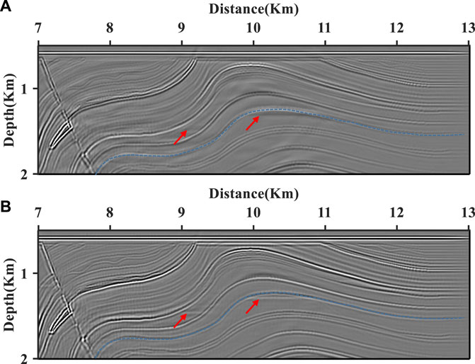
FIGURE 18. The partial enlargements of PP images of the Marmousi 2 model by the scalar imaging condition with the Laplace filter (Panel A) and with the pseudo-Laplace filter (Panel B). The polarity of the event (such as events marked by the blue curve) in Panel B is more continuous than that in Panel A. Furthermore, clearer interfaces and less disturbance of the oil and gas reservoirs at sub-cover (marked by the red arrow), indicated by the partial enlargements of the elastic Marmousi 2 model in Figure 17B, are located in Panel B.

Discussions

The dot product cross-correlation scalar imaging condition, similar to the cross-correlation scalar wave field imaging condition, is a simple and effective imaging condition for vector-based wavefields. Naturally, the PP image by the dot product scalar imaging condition encounters backscattering noise, also being in cross-correlation imaging results, and polarity reversal problem caused by the weighting factor $\cos \theta$. The scalar imaging condition with a pseudo-Laplace filter has been developed as an analogy to the cross-correlation imaging condition with the Laplace filter. Analogous to the cross-correlation imaging condition with the Laplace filter, the scalar imaging condition with pseudo-Laplace filter has been proposed.

Table 1 is the comparative table for the Laplace filter and pseudo-Laplace filter characters from the backscattering noise, the polarity reversal, the spectral variation, and the computation cost. Overall, the pseudo-Laplace filter is similar to the Laplace filter in backscattering suppression, spectral variation, and computation cost. However, it is only the pseudo-Laplace filter that could correct the polarity reversal problem at large incidence. Therefore, the field data with large offset are suitable for the proposed pseudo-Laplace filter. As for the filters composed of second-order spatial derivatives, the angular frequency ${\omega }^2$ has been introduced into the final image. Similar to spectrum modification of a Laplace filter, some low-frequency effective information of the PP image with a pseudo-Laplace filter would be suppressed due to the introduction of ${\omega }^2$. Further study of the low-frequency compensation should be carried out.

TABLE 1

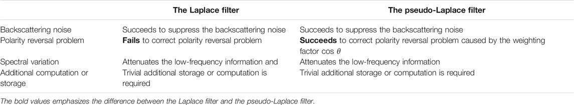
TABLE 1. The comparison between the Laplace filter and pseudo-Laplace filter.

Once the low-frequency information is compensated, the weighting factor ${\left(\cos \theta +1\right)}^2$ can be extracted by deciding the modulus of the incident wave and reflected wave. The weighting factor ${\left(\cos \theta +1\right)}^2$is in a linear relationship with the opening angle. Furthermore, the scalar imaging condition with pseudo-Laplace can be used to extract common imaging point gathers. The SS image by the dot product–based scalar imaging condition suffers from the backscattering and polarity reversal, whose generating mechanism is similar to the PP image. The pseudo-Laplace filter can be extended to the SS image.

Conclusion

The PP image by the dot product–based scalar imaging condition will encounter the problem of polarity reversal when the opening angle exceeds ${90}^{\circ }$ and backscattering noise when the opening angle is close to ${180}^{\circ }$. Based on the application of the Laplace filter for vector-based wavefield, we propose the pseudo-Laplace filter. Unlike the Laplace filter, the scalar imaging condition with a pseudo-Laplace filter only consists of second-order parallel-oriented partial derivatives of Cartesian components cross-correlation results and omits normal-oriented partial derivatives of Cartesian components cross-correlation result. Derivation with plane wave assumption shows that the proposed pseudo-Laplace filter, which depends on the weighting factor ${\left(\cos \theta +1\right)}^2$, can correct polarity reversal and attenuate backscattering artifacts in the PP image. Numerical experiments of the two-layer flat model, four-layer inclined model, and Marmousi 2 model have verified the efficiency and accuracy of the pseudo-Laplace filter. The proposed pseudo-Laplace filter can provide the image with backscattering suppression and continuous phase, which can be further used to extract common imaging point gathers.

Data Availability Statement

The original contributions presented in the study are included in the article/Supplementary Material; further inquiries can be directed to the corresponding authors.

Author Contributions

QD and XZ contributed to the conception and design of the study. SZ organized the database and performed the statistical analysis. FZ and L-YF modified the manuscript. All authors contributed to manuscript revision and read and approved the submitted version.

Funding

This research was supported by the National Science Foundation of China (41930429 and 41774139), the China National “111” Foreign Experts Introduction Plan for Tight Oil & Gas Geology and Exploration, and the Deep-Ultradeep Oil & Gas Geophysical Exploration and Qingdao Applied Research Projects.

Conflict of Interest

The authors declare that the research was conducted in the absence of any commercial or financial relationships that could be construed as a potential conflict of interest.

Publisher’s Note

All claims expressed in this article are solely those of the authors and do not necessarily represent those of their affiliated organizations, or those of the publisher, the editors and the reviewers. Any product that may be evaluated in this article, or claim that may be made by its manufacturer, is not guaranteed or endorsed by the publisher.

Acknowledgments

The authors are grateful to the associate editor H-WZ and reviewers for reviewing this manuscript and Qamar Yasin for revising this manuscript.

References

Aki, K., and Richards, P. (1980). Quantitative Seismology[M]. New York: W. H. Freeman.

Baysal, E., Kosloff, D. D., and Sherwood, J. W. C. (1983). Reverse Time Migration. Geophysics 48 (11), 1514–1524. doi:10.1190/1.1441434

CrossRef Full Text | Google Scholar

Claerbout, J. F. (1971). Toward a Unified Theory of Reflector Mapping. Geophysics 36 (3), 467–481. doi:10.1190/1.1440185

CrossRef Full Text | Google Scholar

Dellinger, J., and Etgen, J. (1990). Wave‐field Separation in Two‐Dimensional Anisotropic media. Geophysics 55 (7), 914–919. doi:10.1190/1.1442906

CrossRef Full Text | Google Scholar

Du, Q., Gong, X., Zhang, M., Zhu, Y., and Fang, G. (2014). 3D PS-Wave Imaging With Elastic Reverse-Time Migration. Geophysics 79 (5), S173–S184. doi:10.1190/geo2013-0253.1

CrossRef Full Text | Google Scholar

Du, Q., Guo, C., Zhao, Q., Gong, X., Wang, C., and Li, X.-y. (2017). Vector-based Elastic Reverse Time Migration Based on Scalar Imaging Condition. Geophysics 82 (2), S111–S127. doi:10.1190/geo2016-0146.1

CrossRef Full Text | Google Scholar

Du, Q. Z., Zhu, Y. T., Zhang, M. Q., and Gong, X. F. (2013). A Study on the Strategy of Low Wavenumber Noise Suppression for Prestack Reverse Time Depth Migration. Chin. J. Geophys. 56 (7), 2391–2401. doi:10.6038/cjg20130725

Google Scholar

Duan, Y., and Sava, P. (2015). Scalar Imaging Condition for Elastic Reverse Time Migration. Geophysics 80 (4), S127–S136. doi:10.1190/geo2014-0453.1

CrossRef Full Text | Google Scholar

Elita Li, Y., Du, Y., Yang, J., Cheng, A., and Fang, X. (2018). Elastic Reverse Time Migration Using Acoustic Propagators. Geophysics 83 (5), S399–S408. doi:10.1190/geo2017-0687.1

CrossRef Full Text | Google Scholar

Lecomte, I. (2008). Resolution and Illumination Analyses in Psdm: A ray-Based Approach. Leading Edge 27 (5), 650–663. doi:10.1190/1.2919584

CrossRef Full Text | Google Scholar

Li, Z. C. (2007). Numeric Simulation of Elastic Wavefield Separation by Staggering Grid High-Order Finite-Difference Algorithm (In Chinese). Oil Geophys. Prospect. 42 (5), 510–515. doi:10.1016/S1872-5813(08)60001-8

Google Scholar

Liu, H. W., Liu, H., Zou, Z., and Cui, Y. F. (2010). The Problem of Denoise and Storage in Seismic Reverse Time Migration (In Chinese): Chinese. J. Geophys. 53 (9), 2171–2180. doi:10.1002/cjg2.1530

CrossRef Full Text | Google Scholar

Ma, D., and Zhu, G. (2003). Numerical Modeling of P-Wave and S-Wave Separation in Elastic Wavefield. Oil Geophys. Prospect. 38 (5), 482–486. doi:10.1007/BF02974893

Google Scholar

Martin, G. S., Wiley, R., and Marfurt, K. J. (2006). Marmousi2: An Elastic Upgrade for Marmousi. The Leading Edge 25 (2), 156–166. doi:10.1190/1.2172306

CrossRef Full Text | Google Scholar

McMechan, G. A. (1983). Migration by Extrapolation of Time-dependent Boundary Values*. Geophys. Prospect 31 (3), 413–420. doi:10.1111/j.1365-2478.1983.tb01060.x

CrossRef Full Text | Google Scholar

Rocha, D., Tanushev, N., and Sava, P. (2016). Isotropic Elastic Wavefield Imaging Using the Energy Norm. Geophysics 81 (4), S207–S219. doi:10.1190/geo2015-0487.1

CrossRef Full Text | Google Scholar

Sun, R., and McMechan, G. A. (1986). Pre-Stack Reverse-Time Migration for Elastic Waves With Application to Synthetic Offset Vertical Seismic Profiles. Proc. IEEE 74 (3), 457–465. doi:10.1109/PROC.1986.13486

Tang, C., and McMechan, G. A. (2018). Multidirectional-vector-based Elastic Reverse Time Migration and Angle-Domain Common-Image Gathers with Approximate Wavefield Decomposition of P- and S-Waves. Geophysics 83 (1), S57–S79. doi:10.1190/geo2017-0119.1

CrossRef Full Text | Google Scholar

Wang, W., and McMechan, G. A. (2015). Vector-based Elastic Reverse Time Migration. Geophysics 80 (6), S245–S258. doi:10.1190/geo2014-0620.1

CrossRef Full Text | Google Scholar

Whitmore, N. D. (1983). Iterative Depth Migration by Backward Time Propagation: SEG Technical Program Expanded Abstracts 1983. Soc. Expl. Geophys., 382–385.

Google Scholar

Xiao, X., and Leaney, W. S. (2010). Local Vertical Seismic Profiling (VSP) Elastic Reverse-Time Migration and Migration Resolution: Salt-Flank Imaging with Transmitted P-To-S Waves. Geophysics 75 (2), S35–S49. doi:10.1190/1.3309460

CrossRef Full Text | Google Scholar

Yan, J., and Sava, P. (2008). Isotropic Angle-Domain Elastic Reverse-Time Migration. Geophysics 73 (6), S229–S239. doi:10.1190/1.2981241

CrossRef Full Text | Google Scholar

Yang, J., Zhu, H., Huang, J., and Li, Z. (2018). 2D Isotropic Elastic Gaussian-Beam Migration for Common-Shot Multicomponent Records. Geophysics 83 (2), S127–S140. doi:10.1190/geo2017-0078.1

CrossRef Full Text | Google Scholar

Yoon, K., and Marfurt, K. J. (2006). Reverse-Time Migration Using the Poynting Vector. Geophys. Explor. 59 (1), 102–107.

Youn, O. K., and Zhou, H. W. (2001). Depth Imaging with Multiples. Geophysics 66 (1), 246–255. doi:10.1190/1.1444901

CrossRef Full Text | Google Scholar

Zhou, X., Chang, X., Wang, Y., and Yao, Z. (2018). Scalar Pp and Ps Imaging of Elastic Rtm by Wavefield Decoupling Method: SEG Technical Program Expanded Abstracts 2018. Soc. Expl. Geophys., 2417–2421. doi:10.1190/segam2018-2995359.1

Google Scholar

Zhu, H. (2017). Elastic Wavefield Separation Based on the Helmholtz Decomposition. Geophysics 82 (2), S173–S183. doi:10.1190/geo2016-0419.1

CrossRef Full Text | Google Scholar

Appendix A: Hadamard Product and its Application

For the vectors s and t with the same dimension, we can obtain a new vector w by the Hadamard product ◦. The new vector $\mathbf{w}$ of Hadamard product, whose element is equal to the element-wise product of vectors s and t, is described as follows:

$\mathbf{w}=\mathbf{s}\circ \mathbf{t}=\left(s_x{t}_x,s_y{t}_y,s_z{t}_z\right).(\mathrm{A1})$

By introducing the Hadamard product into vectors ${\mathbf{s}}^p$ and ${\mathbf{r}}^p$, the imaging vector ${\mathbf{s}}^p°{\mathbf{r}}^p$ at each imaging time can be expressed by the components as follows:

$\left(s_x^p{\overline{r}}_x^p,s_y^p{\overline{r}}_y^p,s_z^p{\overline{r}}_z^p\right).(\mathrm{A2})$