Two-Dimensional Space-Time Image Velocimetry for Surface Flow Field of Mountain Rivers Based on UAV Video

Space-time image velocimetry (STIV) is a promising technique for river surface flow field measurement with the development of unmanned aerial vehicles (UAVs). STIV can give the magnitude of the velocity along the search line set manually thus the application of the STIV needs to determine the flow direction in advance. However, it is impossible to judge the velocity direction at any points before measurement in most mountainous rivers due to their complex terrain. A two-dimensional STIV is proposed in this study to obtain the magnitude and direction of the velocity automatically. The direction of river flow is independently determined by rotating the search line to find the space-time image which has the most prominent oblique stripes. The performance of the two-dimensional STIV is examined in the simulated images and the field measurements including the Xiasi River measurements and the Kuye River measurements, which prove it is a reliable method for the surface flow field measurement of mountain rivers.

Introduction

The flow velocity and discharge are two important hydrological parameters of the mountain flash floods. However, accurate real-time field measurement of the mountain flash floods is often difficult to achieve due to the imperfect infrastructure of the remote mountainous areas and the dangers of the on-site contact measurement. The flow rates and velocities of mountain flash floods are mostly estimated based on the disaster remains currently. Therefore, a non-contact remote velocimetry suitable for the field environment will facilitate the monitoring and research of mountain flash floods.

In recent years, image-based velocimetry such as particle image velocimetry (PIV) and particle tracking velocimetry (PTV) has attracted much attention and recognition due to its convenience of non-contact and ability to obtain the two-dimensional flow fields. Some researchers have developed large-scale PIV and large-scale PTV for the measurement of surface flow fields of rivers and have some successful applications (Tang et al., 2008; Muste et al., 2014; Lewis and Rhoads, 2015; Le Boursicaud et al., 2016; Thumser et al., 2017). Early applications of the LSPIV and LSPTV on the river surface velocity measurement mainly relied on setting up fixed cameras on river banks or bridges, which is especially unsuitable for the measurement of mountain flash floods. Fujita and Hino, 2003, Fujita and Kunita, 2011 used a helicopter-mounted camera to shoot the surface of the river which solved the problem of the need to build fixed camera monitoring facilities, but the cost was too high to be widely applied. With the development of unmanned aerial vehicles (UAVs), UAV has become a more economical and convenient image acquisition equipment with good performance in flexibility and stability for the river measurement. (Eraslan et al., 2020; Kose and Oktay, 2020) Currently, the UAV images are widely used in the measurement of ground topography by the Structure from Motion (SfM) technique (Bakker and Lane, 2017; Lucieer et al., 2014; Woodget et al., 2015) and the measurement of the gravel size distributions by image segmentation techniques (Detert and Weitbrecht, 2012; Westoby et al., 2012). For the surface flow field, some researchers have also begun to use UAV to carry out measurements after the maturity of the UAV fixed-point hovering technique and the video images stabilizing technique (Mied et al., 2018; Tsuji et al., 2018; Koutalakis et al., 2019). The use of UAV will provide great potential convenience for the measurement of mountain flash floods. After receiving the flash flood warning, the operator can take off the UAV from a measurement base several kilometers or even tens of kilometers away from the flash flood site to carry out non-contact measurements, while ensuring both the real-time measurement and personnel safety.

For UAV video processing, the application of LSPTV is greatly limited due to the reliance on artificial release of tracer particles or floating branches and other accidental natural tracers. The fundamental assumption behind LSPIV is that visible texture which is usually the superposition of turbulence-generated surface ripples on the water surface acts as a passive tracer relative to the surface flow. When the effect of wind is negligible, this assumption has been validated in various field measurements (Sun et al., 2010; Chickadel et al., 2011; Tsubaki et al., 2011; Puleo et al., 2012, Al-Mamari et al., 2019). LSPIV measures an instantaneous flow field using a pair of images with a specified time separation. Given that the time separation is usually very short, the accuracy of LSPIV is often severely affected at some river surface areas that lack significant texture. To overcome this shortcoming, Fujita et al. (2007) proposed the space-time image velocimetry (STIV) by using hundreds of continuous images from videos. STIV generates a space-time image by extracting grayscale values on the search line set in the direction of main flow from hundreds of continuous images. The moving textures on the river surface will form oblique stripes on the space-time images. The average velocity during the time period of captured continuous images at the search line can be obtained by extracting the oblique stripes and calculating the inclination. Many researchers Fujita et al. (2019); Zhao et al. (2021); Fujita et al. (2020) evaluated the accuracy of STIV, and found STIV is a technique to measure streamwise velocity distributions more efficiently and accurately compared with LSPIV.

STIV is essentially a one-dimensional velocimetry because it only gives the magnitude of the velocity while the velocity direction depends on the search line. It requires a predetermined velocity direction for setting a search line. It will encounter the problem of determining the direction of velocities when applying the STIV to videos of mountain rivers taken by UAV. Different from the analysis of the fixed camera videos on the river bank, most mountain rivers are meandering and the flow direction changes from place to place thus it is impossible to determine the specific flow direction before measuring. To overcome the shortcoming of STIV, a two-dimensional velocimetry, space-time volume velocimetry (STVV), is proposed by Tsuji et al. (2018). In STVV, the time evolution of image intensity distribution within a rectangular area set on a river surface is expressed as a space-time volume (STV) having three axes with two image coordinate directions and the time direction. The surface velocity vector is obtained by identifying the space angle of the oblique stripes in the STV. Since the recognition of the space angle is more difficult than that of the plane angle, the accuracy of STVV depends heavily on the angle recognition error. In this study, the authors proposed the two-dimensional space-time image velocimetry (2D STIV) for surface flow field of mountain rivers based on UAV videos, which determine the velocity direction by rotating the search line to find the space-time image which has the most prominent oblique stripes. In the following Methods, the algorithm of this two-dimensional velocimetry and the solution to the technical problems of UAV will be presented in detail. In Results and Discussion, the new method is evaluated in simulated images and the field measurements. Finally, the conclusions are summarized in Conclusion.

Methods

The two-dimensional space-time image velocimetry (2D STIV) proposed here is an improved method based on STIV. The magnitude of the velocity in this method is determined by the STIV and the velocity direction is obtained by rotating the search line to find the space-time image which has the most prominent oblique stripes. A brief introduction of STIV is given for the complete description of the 2D STIV, and the details of STIV can be found from Fujita et al. (2007), Fujita et al. (2019).

Magnitude of the Velocity

STIV supposes that different scale turbulent structures in the river interact with the free surface and cause a large number of ripples, boils and bubbles, which produce visible surface textures. The surface textures move with the flows and can be used as tracers to obtain the river surface velocities. In STIV, a search line needs to be set along the flow direction firstly as shown in Figure 1. The red arrow in Figure 1A is the direction of the flow and the red line segment represents the search line for STIV. The grayscale values of each point on the search line from the videos can be extracted and arranged in chronological order then a space-time image is generated as shown in Figure 1B. The vertical length of the space-time image is the same as that of the search line, and the horizontal axis is the number of frames which stands for the time delay. The oblique stripes in the space-time image are produced by the surface textures moving with the flow. The average flow velocity along the search line during the time period can be obtained by calculating the tangent value of the inclination angle. As a result, the key of STIV is to identify the inclination of the stripes on the space-time image. The Eq. 1.1 proposed by Fujita et al. (2019) is used to detect the inclination:

$R\left({\tau }_x,{\tau }_t\right)={\displaystyle {\int }_{-\infty }^{\infty }{\displaystyle {\int }_{-\infty }^{\infty }f\left(x,t\right)f\left(x-{\tau }_x,t-{\tau }_t\right)dxdt}},$(1.1)

where f (x, t) is the grayscale value of the space-time image, (τ_x, τ_t) are the displacement parameters, R (τ_x, τ_t) is the two-dimensional autocorrelation function. R (τ_x, τ_t) will get a relatively large value when (τ_x, τ_t) is along the direction of the stripes on the space-time image. Fourier transform is usually used in the actual calculation and R is normalized. The large R value area will be gathered to the center of the image during this process as shown in Figure 2B. The tilt angle of the large R value area is directly related to the inclination of the stripes in the space-time image in Figure 2B. To identify the tilt angle of the large R area, the coordinate system is converted to a polar coordinate system (see Figure 2C), and absolute R is integrated along polar axis at different angles:

$F\left(\theta \right)={\displaystyle \underset{0}{\overset{\max \left(\rho \right)}{\int }}\left|R\left(\rho ,\theta \right)\right|d}\rho$(1.2)

where

$\max \left(\rho \right)=\min \left(\max \left({\tau }_x\right),\max \left({\tau }_t\right)\right)$(1.3)

R (ρ, θ) is the autocorrelation coefficient under polar coordinate system. F(θ) is the integral value of R (ρ, θ) at different angles. θ is calculated by Eq. 1.4, which means F(θ) will reach a maximum value p when θ equals to the tilt angle of the large R value area, as shown in Figure 2D. The magnitude of the velocity along the search line will be obtained further by involving the frame rate and image spatial resolution of the video after the inclination θ of the stripes on the space-time image is determined.

$\theta =\arg \max \left[F\left(\theta \right)\right]$(1.4)

FIGURE 1

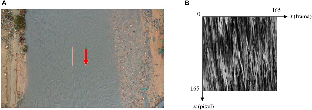
FIGURE 1. Principle of STIV. (A) A search line set along the direction of the river flow. (B) A space-time image generated from the search line.

FIGURE 2

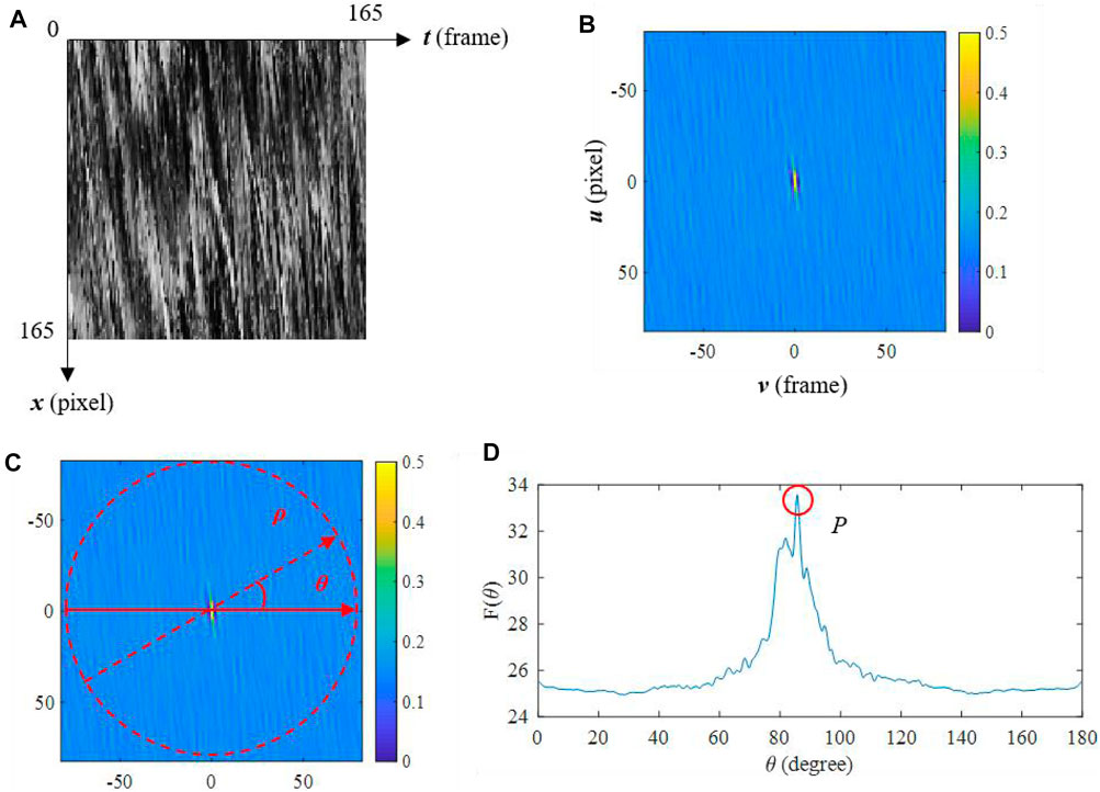
FIGURE 2. Process of obtaining the magnitude of the velocity. (A) An original STI. (B) The autocorrelation coefficient R. (C) A polar coordinate system converted from (B). (D)F (θ) at different angles and p is the maximum value.

Direction of the Velocity

To determine the flow direction, the search line will be rotated around the point to be measured, and then the line with the highest correlation coefficient will be picked out as the direction of velocity. The search line located at the point to be measured is rotated from the horizontal (see Figure 3). We can get a related space-time image at each angle Φ. If the direction of the search line is different from the flow direction at the point to be measured, the surface textures moving with the flow will cross the search line straightly and cannot form remarkable stripes in the space-time images. In contrast, if the direction of the search line is the same as the flow direction, the surface textures will move along the search line for a relatively long time thus form remarkable stripes in the space-time images. Figure 4 shows the space-time images of search lines in Figure 3 at 6 typical angles. It can be seen clearly that there are remarkable oblique stripes in Figure 4A yet the stripes become shorter and blurry as the angle increases. From Figure 3, the main stream direction at the point to be measured should be roughly 0°<Φ<45°, which coincides with the phenomena in Figure 4. Hence, the angle Φ of the search line which makes the stripes most remarkable in the space-time images can be regarded as the velocity direction. In view of the correlation coefficient is the measure of the significance of the oblique stripes in the space-time images, the velocity direction can be determined by comparing the p value for each Φ. Figure 5 plots the p value for 0°<Φ<180°. The rotation angle Φ is calculated by:

$\Phi =\text{argmax}\left(P\right)$(1.5)

Here, Φ = 11.5° so that the velocity direction at this point is 11.5° rotated clockwise from the horizontal. In the space-time image for the search line at 11.5°, the tilt angle of the stripes θ is 59.7°, thus the magnitude of the velocity 1.71 m/s can be obtained from θ by involving the frame rate and image spatial resolution of the video.

FIGURE 3

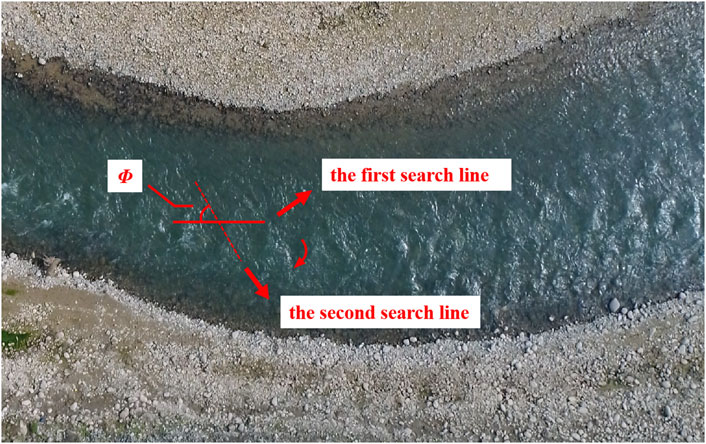
FIGURE 3. A search line is rotated at one point to be measured from the horizontal in a UAV video and the rotating angle is Φ.

FIGURE 4

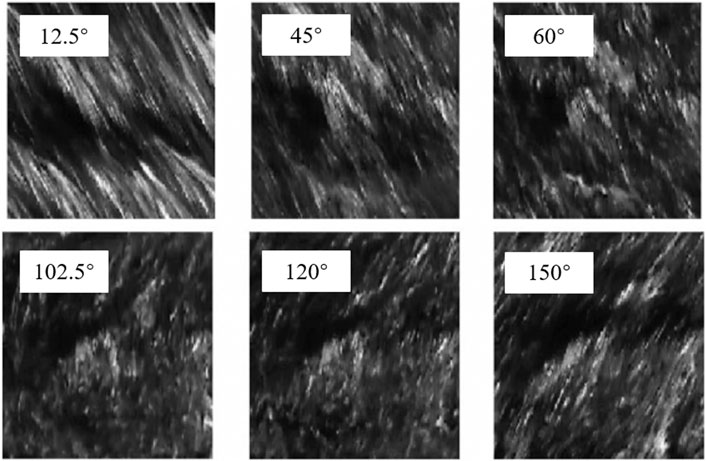
FIGURE 4. The space-time images of search lines at 6 typical angles. (A) 12.5°, (B) 45°, (C) 60°, (D) 102.5°, (E) 120°, (F) 150°.

FIGURE 5

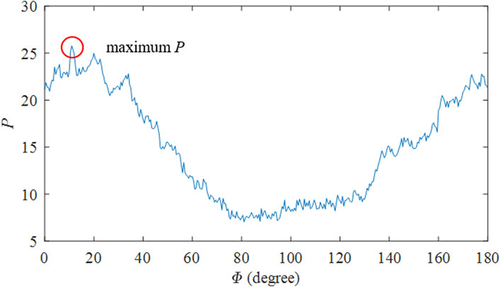
FIGURE 5. the p value for 0°<Φ<180°. The rotation angle Φ corresponding to maximum p is the direction of the flow velocity at this point to be measured.

Results and Discussion

To examine the performance of the proposed method, two-dimensional STIV is applied to simulated images and two UAV videos which were taken from the Xiasi River and the Kuye River. The magnitudes and directions of the velocities in the simulated images are known, thus the accuracy of the 2D STIV can be accurately estimated. The Xiasi River and Kuye River are typical mountain rivers, and the UAV videos from them are used to demonstrate the effect of 2D STIV in practical application. The results of 2D STIV, LSPIV and propeller flow meter are compared to explain the difference between the three methods.

Simulated Images

The simulated image sequences of a river are prepared as shown in Figure 6. A small part of an image is cut out as the object of analysis. Every time the next image is cut out, we will move a certain distance from the last one. Thus, the river surface has a velocity in the combined video. The moving distance along the horizontal and vertical directions is artificially set, so the magnitudes and directions of the velocities in the simulated images are known precisely as shown in Table 1. There are 3 simulated image cases. The magnitudes of the velocities change from 1.41 pixels/frame to 3.16 pixels/frame and the directions change from 45° to 71.57°.

FIGURE 6

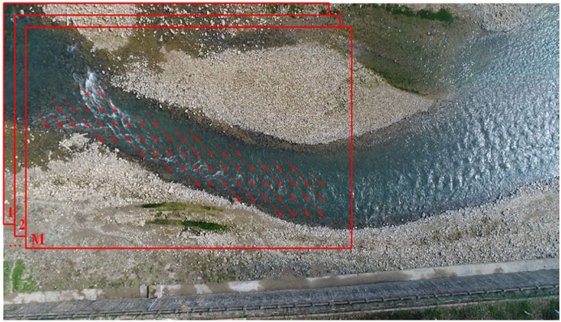
FIGURE 6. Simulated images of river sequence. The Area1 represents a 1760 × 2,425 part on a 2,160 × 3,840 image extracted from the UAV video of the Xiasi River. The AreaM is obtained from Area1 moving m pixels horizontally and n pixels vertically on the frame of image. The red arrows are velocities of the simulated images 1 to M when m is 1 pixel, n is 1 pixel.

TABLE 1

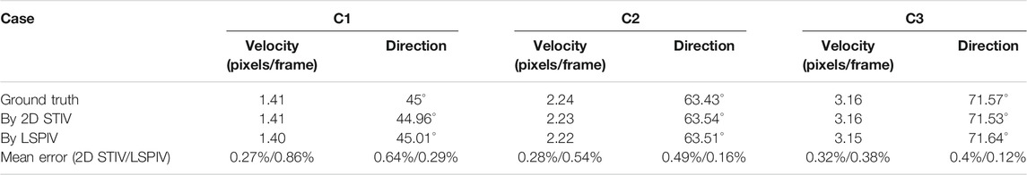
TABLE 1. Results of analyzing simulated images by 2D STIV and LSPIV.

The results including the mean velocity magnitude, direction and error by 2D STIV and LSPIV are listed in Table 1. The biggest error of 2D STIV in velocity magnitude and direction is 0.32% and 0.64% respectively. The error is small enough that the 2D STIV can be considered as an accurate velocity measurement method. It is worth noting that the flow velocity errors of 2D STIV in various cases are less than that of LSPIV, which is similar to the results of other researchers comparing STIV and LSPIV (Muste et al., 2014; Fujita et al., 2019). This is because the information of only two adjacent images is used in each calculation of PIV while multiple pieces are used in 2D STIV at the same time so that the calculation of the average velocity of 2D STIV will be more accurate. However, the reason why the direction errors of LSPIV are smaller than that of 2D STIV is that the 2D STIV depends on the angular resolution when rotating the search line to determine the angle Φ. The direction errors of the 2D STIV will be further reduced as the angular resolution increases. Besides, it can be seen that the error of 2D STIV varies with the flow velocity and direction. In fact, the measurement parameters such as the frame rate and image spatial resolution when shooting the video, the length of the search line and selected frames of the video are all related to error and the final manifestation of these factors is the inclination θ of the stripes in the space-time image and the inevitable error α in the detection of the inclination. The measurement error can be controlled by changing the measurement parameters.

The Xiasi River Measurements

The Xiasi River is located in Guangyuan city, Sichuan Province. It is a typical mountain river at an altitude of 800 m in the upper reaches of the Yangtze river in southwest China. The length of the river reach within the measurement area is about 55 m and the narrowest river width is 4.9 m while the widest is 17.7 m. The measurements were conducted in October 2018. There was no wind and the temperature was 16°C on the day of measurement.

The UAV video was taken by a DJI Mavic 2. Table 2 lists the specifications of the UAV. The selected frame rate of the video was 60 fps. When capturing the videos, the UAV was hovering stably and shooting the river surface from a perpendicular view. The affine transformation was utilized to stabilize the video. There will be jitters of the image sequence due to the shaking of UAV in the wind. All measurements were carried out in a windless or breezy weather to avoid large-scale jitter in the UAV video. The affine transformation is utilized to eliminate the remaining inevitable jitters. The specific process of affine transform is:

1) Pick at least four ground control points (GCPs) on the river bank which have distinctive features and unchanged characteristic on the first image of the video;

2) The areas at GCPs of each image in video is cross-correlated with the first image to obtain the displacements of GCPs in each image;

3) Calculate the affine transformation matrixes between the first image and other images according to the displacements of GCPs;

4) The affine transformation matrixes are used to transform each image, so that the coordinates of the GCPs in each image are unchanged.

TABLE 2

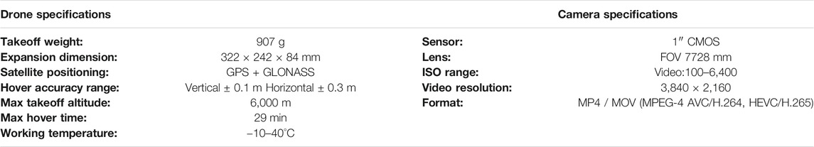
TABLE 2. The DJI Mavic2 specifications (from https://www.dji.com).

In the 2D STIV analysis, 201 frames (3.35 s) are used and the length of a search line is 165 pixels. The image spatial resolution is 60 pixels/m, thus the grid spacing of vectors is 2 m. The step of rotation angle Φ was taken as 0.5° thus the resolution of velocity direction is 0.5°. The calculated results are shown in Figure 7. It can be seen that the main flow directs to the lower right in the left half image and the upper right in the right half image when checking the velocity direction carefully. The velocity directions are correct in generally as the river is U-shaped. In addition, there is a backflow area in the upper right part of the image, and part of the flow in the mainstream will enter the backflow area. The enlarged view in Figure 7 shows that the velocity vectors reflect the backflow phenomenon well in the backflow area.

FIGURE 7

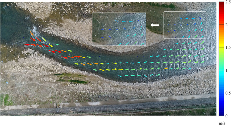
FIGURE 7. Flow field of Xiasi river surface from the UAV video using 2D STIV. The color and length of the velocity arrows. The grid spacing is 2 m.

In order to verify the numerical results by 2D STIV, LSPIV analysis was also applied for this video. The grid spacing of vectors is 0.83 m and other parameters remains in 2D STIV. Flow fields obtained by these two methods with the same parameters and grid coordinate system for comparison are shown in Figure 8. As can be seen from the figure, the general results of the two methods are consistent. We performed statistical analysis on the velocity vectors at the same position of the two methods, and found that the average absolute difference of the flow velocity calculated by 2D STIV and LSPIV is 0.3477 pixels/frame and the standard deviation is 0.1002 pixels/frame, and the average absolute difference of flow directions is 6.2408° and the standard deviation is 2.5401°.

FIGURE 8

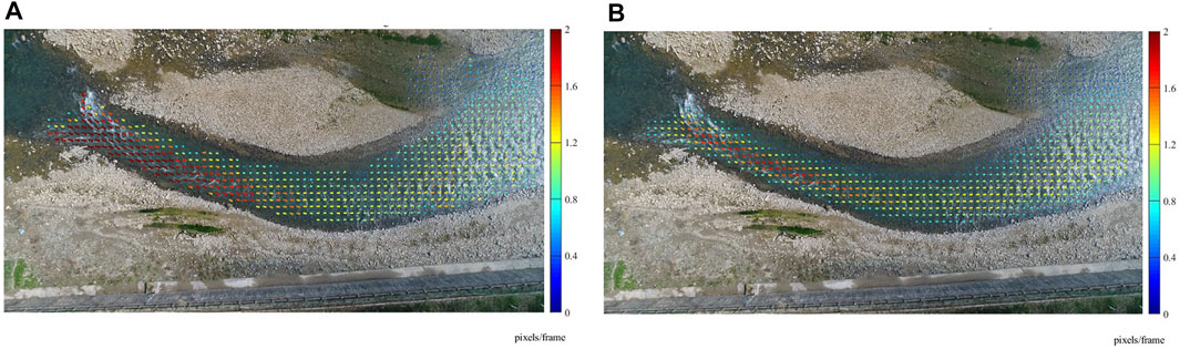
FIGURE 8. Flow fields obtained by the two methods at the same grid coordinate system. (A) Flow field of the Xiasi River surface from the UAV video using 2D STIV. (B) Flow field of the Xiasi River surface from the UAV video using LSPIV.

The Kuye River Measurements

The Kuye River is located in Yulin city, Shanxi Province. It is a typical mountain river in the middle reaches of the Yellow river in northwest China. The altitude of the measurement location is about 1,100 m. The UAV videos were taken in September 2019. The measurement day was breeze, light to moderate rain, and the temperature was 20°C. The selected frame rate of the videos was 24 fps. The affine transformation was also utilized to stabilize the video. The length of the search line is 165 pixels and 165 frames (5.5 s). The image spatial resolution of this video is 300 pixels/m, thus the grid spacing of vectors is 0.67 m. The resolution of velocity direction is also 0.5°. The velocity distribution by the two-dimensional STIV are shown in Figure 9 indicating that the velocity is relatively low near the bank while is relatively high in the center of the river, and the typical velocity is about 1m/s. The maximum velocity is 2.36 m/s and located at the lower border of the image due to the interference of stones downstream. The results above are consistent with the experience of on-site visual observation.

FIGURE 9

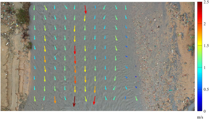
FIGURE 9. Velocity distribution derived from the Kuye River surface based on UAV video using two-dimensional STIV. The color and length indicate magnitude of the velocity. Grid spacing of vectors is 0.67 m.

The average width of the river is about 10 m, and the water depth is relatively shallow, thus it is possible to operate hand-held device measurement to measure the river surface velocity for comparison (Figure 10A). The manual measurement was carried out at 6 points of a cross-section by Jinshuihuayu LS300A propeller flow meter. The Jinshuihuayu LS300A propeller flow meter demands to judge the velocity direction manually in advance and its velocity band is 0.01∼4 m/s. Moreover, the measurement error is less than or equal to 1.5%. The station pole is placed 0.45 m underwater during the measurement. The UAV videos shooting and the propeller flow meter measuring were conducted simultaneously. The duration of the whole measurement was less than half an hour, so it can be considered that the flow rate of the river and other conditions remained unchanged during the entire measurement period. The cross-section and the specific measurement points are shown in Figure 10B. The 6 measurement positions were set at 1.2, 2.4, 3.6, 4.8, 6, and 7.2 m away from the control point on the right bank of the river, respectively. Six search lines were set at the same positions to yield the results by the 2D STIV. The results by propeller flow meter and by 2D STIV are provided in Table 3 and Figure 11. The difference is less than 0.24 m/s (minor difference can be understandable given that the propeller flow meter is used below the water surface while results by 2D STIV are surface velocities) except for the first point, which is 0.35 m/s. There are two main reasons for the large error of the first point. Firstly, there had been raining during the measurement making it impossible for surveyors to control the position of the measurement point very accurately. The estimated error is at least 0.5 m for the measurement position. Secondly, the propeller flow meter demands to judge the velocity direction manually but the velocity direction is affected by the bed topography seriously near the river bank and not necessarily parallel to the bank. If there are errors in the determination of velocity direction, it will have a great impact on the velocity magnitude from the propeller flow meter. Regarding these two factors may also affect the other 5 points, the error of the 2D STIV is less than 0.24 m/s here in fact.

FIGURE 10

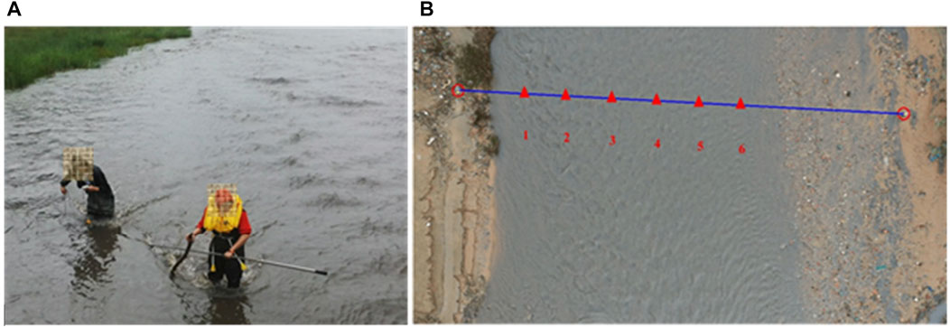
FIGURE 10. Manual measurement by propeller flow meter. (A) Scene of manual measurement. Two people cooperate to determine the points to be measured, one of whom holds a propeller flow meter to measure the surface velocity. (B) Cross-section and measurement positions. The red triangles 1–6 represent the measurement positions 1.2, 2.4, 3.6, 4.8, 6, and 7.2 m away from the right bank of the river, respectively.

TABLE 3

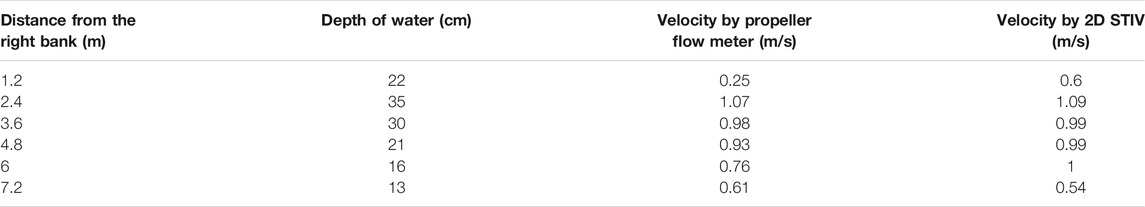
TABLE 3. Results of propeller flow meter and 2D STIV.

FIGURE 11

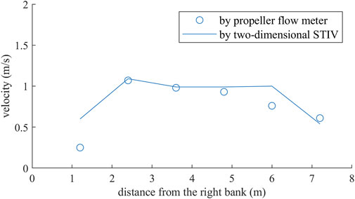
FIGURE 11. Comparison of the results by propeller flow meter and 2D STIV.

Conclusion

An improved STIV method, 2D STIV, is proposed to overcome the shortcomings of the STIV, which needs velocity direction information before measurement. The method determines the velocity direction by rotating the search line to find the space-time image which has the most prominent oblique stripes. The performance of the 2D STIV is examined in simulated images and the field measurements. All results prove the method is reliable so it can be an alternative method in the future. The conclusions can be summarized as follows:

1) When the direction of the search line is the same as the flow direction, the surface textures will move along the search line for a relatively long time and form the most significant stripes in the space-time images. The autocorrelation coefficient of space-time image can be used as the measure of significance of the stripes. Hence, the velocity direction can be determined by rotating the search line to find the space-time image which has the most prominent oblique stripes based on the autocorrelation coefficient.

2) The 2D STIV was applied to analyze the simulated image sequences of a river and are compared with LSPIV. Since the actual velocity and direction are known, the error of two methods can be calculated and compared. The biggest error of 2D STIV in velocity magnitude and direction is 0.32% and 0.64% respectively, which are small enough and the flow velocity errors of 2D STIV in various cases are less than that of LSPIV.

3) The 2D STIV was applied to analyze the UAV videos taken from the Xiasi River and compared with LSPIV. Firstly, it can obtain the correct flow direction from the curved river case. Secondly, the average absolute difference of the flow velocity calculated by 2D STIV and LSPIV is 0.3477 pixels/frame and the standard deviation is 0.1002 pixels/frame, and the average absolute difference of flow directions is 6.2408° and the standard deviation is 2.5401°.

4) The 2D STIV was applied to analyze the UAV videos taken from the Kuye River and compared with the propeller flow meter. The results show that the difference between them is less than 0.24 m/s. Considering the results of propeller flow meter also exist errors, the measurement accuracy of 2D STIV is relatively high.

Data Availability Statement

The raw data supporting the conclusion of this article will be made available by the authors, without undue reservation.

Author Contributions

QZ contributed to conception and design of the study. XH and KC implemented the computer code. KC, QC and QZ finished the field experiments. XH and KC performed the data analysis. XH wrote the first draft of the manuscript. QZ, KC, FW, and DL wrote sections of the manuscript. All authors contributed to manuscript revision, read, and approved the submitted version.

Funding

The study was supported by the National Natural Science Foundation of China (Grant no. 51809268) and the Research Fund Program of Tsinghua–Ningxia Yinchuan Joint Institute of Internet of Waters on Digital Water Governance (Grant no. SKL-IOW-2020TC2007).

Conflict of Interest

The authors declare that the research was conducted in the absence of any commercial or financial relationships that could be construed as a potential conflict of interest.

Acknowledgments

The authors would like to thank Prof. Niannian Fan (State Key Laboratory of Hydraulics and Mountain River Engineering, Sichuan University) for assisting in UAV video capture and field measurement.

References

Al-Mamari, M., Kantoush, S., Kobayashi, S., Sumi, T., and Saber, M. (2019). Real-time Measurement of Flash-Flood in a Wadi Area by LSPIV and STIV. Hydrology 6 (1), 27. doi:10.3390/hydrology6010027

CrossRef Full Text | Google Scholar

Bakker, M., and Lane, S. N. (2017). Archival Photogrammetric Analysis of River-Floodplain Systems Using Structure from Motion (SfM) Methods. Earth Surf. Process. Landforms 42 (8), 1274–1286. doi:10.1002/esp.4085

CrossRef Full Text | Google Scholar

Chickadel, C. C., Talke, S. A., Horner-Devine, A. R., and Jessup, A. T. (2011). Infrared-based Measurements of Velocity, Turbulent Kinetic Energy, and Dissipation at the Water Surface in a Tidal River. IEEE Geosci. Remote Sensing Lett. 8 (5), 849–853. doi:10.1109/lgrs.2011.2125942

CrossRef Full Text | Google Scholar

Detert, M., and Weitbrecht, V. (2012). Automatic Object Detection to Analyze the Geometry of Gravel Grains-Aa Free Stand-Alone Tool. London: Taylor \& Francis Group, 595–600.

Eraslan, Y., O Zen, E., and Oktay, T. U. G. R. (2020). A Literature Review on Determination of Quadrotor Unmanned Aerial Vehicles Propeller Thrust and Power Coefficients, 1–12.

Fujita, I., and Hino, T. (2003). Unseeded and Seeded PIV Measurements of River Flows Videotaped from a Helicopter. J. Vis. 6 (3), 245–252. doi:10.1007/bf03181465

CrossRef Full Text | Google Scholar

Fujita, I., and Kunita, Y. (2011). Application of Aerial LSPIV to the 2002 Flood of the Yodo River Using a Helicopter Mounted High Density Video Camera. J. Hydro-Environment Res. 5 (4), 323–331. doi:10.1016/j.jher.2011.05.003

CrossRef Full Text | Google Scholar

Fujita, I., Notoya, Y., Tani, K., and Tateguchi, S. (2019). Efficient and Accurate Estimation of Water Surface Velocity in STIV. Environ. Fluid Mech. 19 (5), 1363–1378. doi:10.1007/s10652-018-9651-3

CrossRef Full Text | Google Scholar

Fujita, I., Shibano, T., and Tani, K. (2020). Application of Masked Two-Dimensional Fourier Spectra for Improving the Accuracy of STIV-Based River Surface Flow Velocity Measurements. Meas. Sci. Technol. 31 (9), 094015. doi:10.1088/1361-6501/ab808a

CrossRef Full Text | Google Scholar

Fujita, I., Watanabe, H., and Tsubaki, R. (2007). Development of a Non‐intrusive and Efficient Flow Monitoring Technique: The Space‐time Image Velocimetry (STIV). Int. J. River Basin Manag. 5 (2), 105–114. doi:10.1080/15715124.2007.9635310

CrossRef Full Text | Google Scholar

Kose, O., and Oktay, T. (2020). Simultaneous Quadrotor Autopilot System and Collective Morphing System Design. Aircraft Engineering and Aerospace Technology. doi:10.30518/jav.788938

CrossRef Full Text

Koutalakis, P., Tzoraki, O., and Zaimes, G. (2019). UAVs for Hydrologic Scopes: Application of a Low-Cost UAV to Estimate Surface Water Velocity by Using Three Different Image-Based Methods. Drones 3 (1), 14. doi:10.3390/drones3010014

CrossRef Full Text | Google Scholar

Le Boursicaud, R., Pénard, L., Hauet, A., Thollet, F., and Le Coz, J. (2016). Gauging Extreme Floods on YouTube: Application of LSPIV to home Movies for the post-event Determination of Stream Discharges. Hydrol. Process. 30 (1), 90–105. doi:10.1002/hyp.10532

CrossRef Full Text | Google Scholar

Lewis, Q. W., and Rhoads, B. L. (2015). Resolving Two‐dimensional Flow Structure in Rivers Using Large‐scale Particle Image Velocimetry: An Example from a Stream confluence. Water Resour. Res. 51 (10), 7977–7994. doi:10.1002/2015wr017783

CrossRef Full Text | Google Scholar

Lucieer, A., Jong, S. M. d., and Turner, D. (2014). Mapping Landslide Displacements Using Structure from Motion (SfM) and Image Correlation of Multi-Temporal UAV Photography. Prog. Phys. Geogr. Earth Environ. 38 (1), 97–116. doi:10.1177/0309133313515293

CrossRef Full Text | Google Scholar

Mied, R. P., Chen, W., Smith, G. B., Wagner, E. J., Miller, W. D., Snow, C. M., et al. (2018). Airborne Remote Sensing of Surface Velocities in a Tidal River. IEEE Trans. Geosci. Remote Sensing 56 (8), 4559–4567. doi:10.1109/tgrs.2018.2826366

CrossRef Full Text | Google Scholar

Muste, M., Hauet, A., Fujita, I., Legout, C., and Ho, H.-C. (2014). Capabilities of Large-Scale Particle Image Velocimetry to Characterize Shallow Free-Surface Flows. Adv. Water Resour. 70, 160–171. doi:10.1016/j.advwatres.2014.04.004

CrossRef Full Text | Google Scholar

Puleo, J. A., McKenna, T. E., Holland, K. T., and Calantoni, J. (2012). Quantifying Riverine Surface Currents from Time Sequences of thermal Infrared Imagery. Water Resour. Res. 48 (1). doi:10.1029/2011wr010770

CrossRef Full Text | Google Scholar

Sun, X., Shiono, K., Chandler, J. H., Rameshwaran, P., Sellin, R. H. J., and Fujita, I. (2010). Discharge Estimation in Small Irregular River Using LSPIV. Proc. Inst. Civil Eng. - Water Manag. 163, 247–254. doi:10.1680/wama.2010.163.5.247

CrossRef Full Text | Google Scholar

Tang, H.-w., Chen, C., Chen, H., and Huang, J.-t. (2008). An Improved PTV System for Large-Scale Physical River Model. J. Hydrodyn 20 (6), 669–678. doi:10.1016/s1001-6058(09)60001-9

CrossRef Full Text | Google Scholar

Thumser, P., Haas, C., Tuhtan, J. A., Fuentes-Pérez, J. F., and Toming, G. (2017). RAPTOR-UAV: Real-Time Particle Tracking in Rivers Using an Unmanned Aerial Vehicle. Earth Surf. Process. Landforms 42 (14), 2439–2446. doi:10.1002/esp.4199

CrossRef Full Text | Google Scholar

Tsubaki, R., Fujita, I., and Tsutsumi, S. (2011). Measurement of the Flood Discharge of a Small-Sized River Using an Existing Digital Video Recording System. J. Hydro-Environment Res. 5 (4), 313–321. doi:10.1016/j.jher.2010.12.004

CrossRef Full Text | Google Scholar

Tsuji, I., Tani, K., Fujita, I., and Notoya, Y. (2018). Development of Aerial Space Time Volume Velocimetry for Measuring Surface Velocity Vector Distribution from Uav. EDP Sciences, 6011.

Westoby, M. J., Brasington, J., Glasser, N. F., Hambrey, M. J., and Reynolds, J. M. (2012). 'Structure-from-Motion' Photogrammetry: A Low-Cost, Effective Tool for Geoscience Applications. Geomorphology 179, 300–314. doi:10.1016/j.geomorph.2012.08.021

CrossRef Full Text | Google Scholar

Woodget, A. S., Carbonneau, P. E., Visser, F., and Maddock, I. P. (2015). Quantifying Submerged Fluvial Topography Using Hyperspatial Resolution UAS Imagery and Structure from Motion Photogrammetry. Earth Surf. Process. Landforms 40 (1), 47–64. doi:10.1002/esp.3613

CrossRef Full Text | Google Scholar

Zhao, H., Chen, H., Liu, B., Liu, W., Xu, C.-Y., Guo, S., et al. (2021). An Improvement of the Space-Time Image Velocimetry Combined with a New Denoising Method for Estimating River Discharge. Flow Meas. Instrumentation 77, 101864. doi:10.1016/j.flowmeasinst.2020.101864

CrossRef Full Text | Google Scholar