 Thomas Loriaux
 Lucas Ruiz
- 1Centro de Estudios Científicos, Valdivia, Chile
- 2Instituto Argentino de Nivología, Glaciología y Ciencias Ambientales (IANIGLA), Gobierno de Mendoza, Universidad Nacional de Cuyo, CONICET, Mendoza, Argentina
Known for their important role in locally enhancing surface melt, supraglacial ponds and ice cliffs are common features on debris-covered glaciers. We use high resolution satellite imagery to describe pond-cliff systems and surface velocity on Verde debris-covered glacier, Monte Tronador, and Southern Chile. Ponds and ice cliffs represent up to 0.4 and 2.7% of the glacier debris-covered area, respectively. Through the analyzed period and the available data, we found a seasonality in the number of detected ponds, with larger number of ponds at the beginning of the ablation season and less at the end of it. Using feature tracking, we determined glacier surface velocity, finding values up to 55 m/yr on the upper part of the debris-covered area, and decreasing almost to stagnation in the terminus. We found that larger ponds develop in glacier zones of low velocity, while zones of high velocity only contain smaller features. Meanwhile, ice cliffs appeared to be less controlled by surface velocity and gradient. Persistent ice cliffs were detected between 2009 and 2019 and backwasting up to 24 m/yr was measured, highlighting significant local glacier wastage.
Introduction
Interest has been recently growing about debris-covered glaciers (DCGs) in mountain areas worldwide (e.g., Fyffe et al., 2012; Janke et al., 2015; Bhushan et al., 2018; Miles et al., 2019). Main objectives generally consist in assessing the effect of the debris layer on the mass balance (Brock et al., 2007; Hagg et al., 2008; Collier et al., 2015) and their hydrological role in glacierised landscapes (Ayala et al., 2016; Burger et al., 2019; Fyffe et al., 2019; Immerzeel et al., 2020; Miles et al., 2020).
Supraglacial ponds are common features on DCGs, where they have been observed for decades (Iwata et al., 1980; Kirkbride, 1993). Studies about supraglacial ponds on DCGs are mostly centered in High Mountain Asia (e.g., Sakai and Fujita, 2010; Miles et al., 2018; Watson et al., 2018a; Chand and Watanabe, 2019), where they can locally represent significant portion of the DCGs. Seasonal and interannual variations in ponds count and area have been observed (Steiner et al., 2019), as well as rapid filling and draining (Miles et al., 2017b), associated with englacial hydrological networks (Miles et al., 2017a; Miles et al., 2019; Watson et al., 2018b). Ponds also regulate DCGs runoff, as they act as buffer reservoirs (Irvine-Fynn et al., 2017). Exposed ice cliffs often appear at the ponds margins and can help identify the emplacement of drained features (Miles et al., 2017a).
Ponds and ice cliffs are known for their important role in locally enhancing surface melt (Sakai et al., 2000; Benn et al., 2012; Salerno et al., 2012; Maurer et al., 2016), as they absorb and transfer atmospheric energy into the glacier ice (Sakai et al., 2002; Steiner et al., 2015; Brun et al., 2018; Miles et al., 2018). This induces the DCGs to lose as much mass as debris-free glaciers despite the debris layer, which is known as the “debris-cover anomaly” (Pellicciotti et al., 2015; Brun et al., 2018; Bisset et al., 2020). Based on energy balance modeling and satellite-based pond distribution, Miles et al. (2018) estimate that supraglacial ponds contribute to 12 ± 2% of the total ice mass loss in Langtang catchment, Nepal. Thompson et al. (2016) and Reid and Brock (2014) found that ice cliff covering only 5 and 1.3% of glacier surface contribute to 40 and 7.4% of the ablation on DCGs, respectively, in the Himalaya and Alps. Similarly, Brun et al. (2018) found that ice cliffs have a net ablation rate 3.1 ± 0.6 times higher than the average glacier tongue surface. Also, ponds are likely to coalesce and form large glacial lakes, enhancing glacier calving (Chikita et al., 1998; Röhl, 2008; Sakai and Fujita, 2010) and increasing glacial lake hazards (Quincey et al., 2007).
Mapping and inventorying supraglacial ponds and ice cliffs is therefore important due to their role as ablation hotspot and their link with the englacial hydrological network. Understanding of their magnitude and spatio-temporal variation will become increasingly significant on glaciers with negative mass balances (Deline, 2005; Stokes et al., 2007; Benn et al., 2012; Thakuri et al., 2014; Tielidze et al., 2020). In this context of glacier shrinking, mountain ranges are thought to show some transition from debris-free to debris-covered and rock glaciers, with an increase of their relative importance on the freshwater availability, quality and timing (Anderson et al., 2018; Knight et al., 2019).
The present study depicts the first assessment of supraglacial ponds and ice cliffs distribution on a DCG in Chile. Our objectives are to: 1) Document interannual changes in ponds and ice cliffs distribution using Google Earth historical imagery. 2) Analyse the inventory by determining horizontal velocity through feature tracking and extracting surface gradient from digital elevation model (DEM). 3) Detect persistent ice cliffs and measure the associate backwasting.
Regional Context and Area of Interest
The Southern Andes cover more than 4,500 km from northernmost Chile to the southern tip of South America in Tierra del Fuego. The extensive latitudinal range from subtropical to subantarctic domains (20°–55°S), steep elevation gradients, and the north-south orientation perpendicular to the prevalent atmospheric circulation cause significantly different climatic conditions, and consequently, a great variety of ice mass types along the Southern Andes (Lliboutry, 1998). North of 35 S, knows as the Dry Andes, encompasses a high (3,500–6,900 m a.s.l.) mountain range with arid (<500 mm/yr) condition to the north and modest annual precipitation amounts (1,000 mm/yr) to the south (Viale et al., 2019). Due to the topographic relief, geological context, and climatic setting, this region hosts the largest debris-covered glacier area of the Southern Andes (Barcaza et al., 2017; Zalazar et al., 2020). This region also contains the largest concentration of rock glaciers in the Andes (Barcaza et al., 2017), and includes many complex units that start as clean-ice glaciers at high elevations, gradually turn into debris-covered glaciers further down, and finally end as rock glaciers at the lowest sectors (Monnier and Kinnard, 2015, Monnier and Kinnard, 2017; Zalazar et al., 2020). Recent inventories of the Argentina side of this region found that between 60 and 70% of the glacierised area (1,200 km2; excluding rock glaciers) are partially (10%) to totally (˃90%) debris-covered (Ferri et al., 2020).
South of the 35°S, in the Wet Andes, where the elevation of most peaks usually does not exceed 4,000 m a.s.l., the precipitation amounts increase considerably, exceeding 2,000 mm/yr (Viale et al., 2019). Although, at the southern part of this regions the topographic and climatological conditions allow the development of numerous and extensive glacierized areas, which constitute the largest glacierized surface in South America. In the north part, also known as the North Patagonian Andes (35° to 45°S), glaciers are smaller than those located further south. Although glaciers along this region are mainly clean ice or debris free (98% of the glaciated area), debris-covered glaciers can still be found due to local conditions such as rock-fall and stagnation. This is the case of Verde and other valley glaciers at Monte Tronador, where rock-falls and avalanches below a massive bedrock cliff present between 1,700 and 1,400 m a.s.l., allow the concentration of debris over the glaciers tongues (Ruiz et al., 2017).
The seasonal variation in the North Patagonian Andes is driven by the location and intensity of the southern hemisphere westerlies (Garreaud et al., 2009), which bring abundant precipitations between April and September (Aravena and Luckman, 2009). At these latitudes, orographic effect induces an increase of the annual mean precipitation from the Pacific coast to the western slopes of Chile, where it reaches more than 3,000 mm (Viale and Garreaud, 2015). Ruiz et al. (2015) measured more than 3,000 mm w.e. between May and September 2013 on a stake located close to the ice divide between Alerce and Castaño Overa glaciers, and close to the equilibrium-line altitude (ELA), which lies at 2000 m a.s.l. (Carrasco et al., 2005; Condom et al., 2007).
Verde glacier (8.15 km2, 41.21°S, 71.91°W, Table 1) lies on the southern flank of Monte Tronador (3,475 m a.s.l.), an extinct stratovolcano located in the North Patagonian Andes on the Chile-Argentina border (Figure 1). The glacier is divided into three distinct parts: the accumulation zone on the upper slope of the Monte Tronador between 2,500 and 3,475 m a.s.l. an icefall between 1,400 and 2,500 m a.s.l. and a debris-covered tongue down to 980 m a.s.l. The debris-covered tongue is about 3.05 km2, which makes Verde glacier one of the most extended DCGs in Chile (Barcaza et al., 2017).
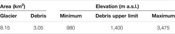
TABLE 1. Characteristics of Verde glacier, including the area of the whole glacier and the debris cover.
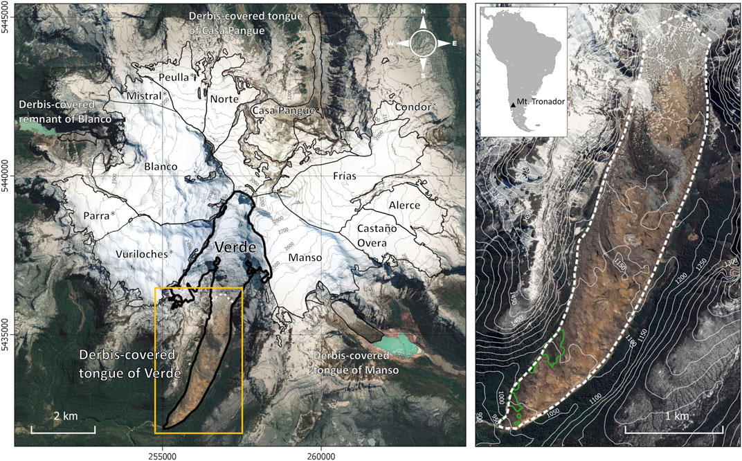
FIGURE 1. Optical CNES/Airbus image of Monte Tronador from October 17, 2019. Verde glacier is delimited by the thick black line while other individual glaciers are delineated by thin black lines. White dotted line on Verde tongue marks the upper limit of the debris cover. Orange rectangle corresponds to the right panel, zooming in the debris-covered tongue of Verde glacier. The presence of some vegetation at the glacier lower part is indicated by green outline polygons. Coordinates in meters, universal transverse mercator (UTM) projection, zone 19, World Geodetic System (WGS84) datum.
Verde glacier has not shown significant retreat or advance over the last decades (Reinthaler et al., 2019), and its terminus is still in contact with the Little Ice Age moraines (Ruiz et al., 2015), which contrasts with the fast retreating behaviour of the glaciers in the region (Paul and Mölg, 2014). Between 2000 and 2012, the Verde glacier has a neutral mass balance (−0.08 ± 0.09 m w.e./yr), which contrast with the negative mass balance of Manso (−0.5 ± 0.1°m w.e./yr) and Casa Pangue (−0.29 ± 0.1 m w.e./yr), the other debris-covered valley glaciers at Monte Tronador (Figure 1). Meanwhile, the most considerable ice thickness changes of the Manso and Casa Pangue glaciers are concentrated in their lower debris-covered tongues. The Verde glacier’s lower part does not show significant elevation change between 2000 and 2012 (mean elevation change of −0.6 ± 0.5 m; Ruiz et al., 2017). By applying cross-correlation to Pléiades satellite images, Ruiz et al. (2015) measured surface displacements over Monte Tronador glaciers between March and June 2012. They found that these glaciers follow a radial flow pattern. At Verde glacier, maximum surface speeds of <390 m/yr were estimated on the steep icefall area. Meanwhile, the lower reaches of the debris-covered tongues of Verde and Casa Pangue glaciers are almost stagnant. They found that low-elevation debris-covered glacier tongues show increasing velocities at the beginning of the accumulation season, probably in response to an increase in water input to the subglacial system from winter rainfall events at low elevations and a decrease in meltwater production at higher elevations.
Recently, Zorzut et al. (2020) calculated the ice thickness distribution of Monte Tronador glaciers and found that the gently sloped debris-covered tongue of the Verde glacier is one of the thicker parts of the whole glaciers of Monte Tronador, with a maximum estimated thickness of around 180 ± 60 m and a total volume of 0.59 ± 0.2 km3.
Material and Methods
Google Earth Imagery
The Google Earth platform freely gives access to optical imagery of high spatial resolution, from SPOT and DigitalGlobe (e.g., QuickBird, Worldview-1 and 2, and IKONOS), and orthorectified based on the DEM from the Shuttle Radar Topography Mission–SRTM (Schmid et al., 2015). Moreover, Google Earth provides an historical catalogue with sufficient temporal resolution to enable investigation of interannual processes. Google Earth has thus been widely used as a main or supporting tool when performing cryosphere-related inventories, mainly of rock glaciers (Rangecroft et al., 2014; Schmid et al., 2015; Nagai et al., 2016; Charbonneau and Smith, 2018; Jones et al., 2018; Pandey, 2019), but also debris-free (Tielidze et al., 2020) and debris-covered glaciers (Alifu et al., 2016a,b), as well as glacial lakes (Wilson et al., 2018).
In the present study, the debris-covered tongue of Verde glacier is analysed with eight high resolution scenes (<0.5 m), whose acquisition dates range from November 2009 to October 2019 (Table 2). Although the image distribution is uneven over the year, the dataset contains three images from end of summer (March 2012, March 2016, and March 2018), one from end of winter (September 2015), as well as four from spring and start of summer (November 2009, December 2012, November 2013, and October 2019). The scenes present clear atmospheric conditions, mostly snow-free, and show limited areas of shadow. Error in horizontal positioning between images will be assessed by marking non-moving features, such as outcrops and trees, outside of the glacier area. No image processing was performed for interpretation.
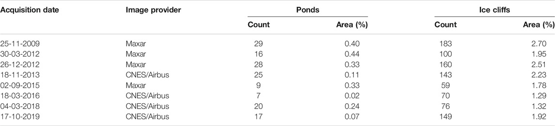
TABLE 2. Ponds and ice cliffs observations for the 3.05 km2 debris-covered tongue of Verde glacier.
Ponds and Ice Cliffs Inventory
The inventory was conducted following the method employed by Bhushan et al. (2018), who analysed high-resolution imagery from Google Earth to identify supraglacial ponds and ice cliffs for 10 DCGs in the Zanskar Basin of Western Himalaya. By-eye ponds and ice cliffs identification and manual digitisation were realised directly in the Google Earth platform through the built-in geographic information system. The ponds and ice cliffs polygons were then exported into the QGIS geographic information system software where their distribution and geometric properties were assessed. Regarding the ice cliffs, the inventory records the planimetric area. Error in area determination was estimated by multiplying feature perimeter by the spatial resolution (Casassa et al., 2014), here rounded at 0.5 m.
The inventory allowed the tracking of persistent ice cliffs over the study period to assess retreat, which is defined here, as the observed distance between the same ice cliff between the initial and the final satellite scenes, divided by the time interval. In order to remove the displacement due to glacier flow and to only assess backwasting due to ablation, the observed ice cliff retreat was corrected for the local mean surface velocity (Steiner et al., 2019). Discriminating between the observed retreat and the assessed backwasting is particularly important for ice cliff retreat occurring parallel to flow direction, in which case the difference is maximum.
Glacier Characteristics
Horizontal surface velocity was determined following the method described by Immerzeel et al. (2014) and Wigmore and Mark (2017), who manually tracked topographic features on high-resolution photographs acquired using unmanned aerial vehicles. In the present study, this approach was adapted by tracking evenly spaced and clearly distinguishable boulders, at the glacier surface using the Google Earth historical imagery (Figure 2). For each identified boulder, a vector was drawn using the Google Earth path tool, which each node corresponded to the boulder position at the respective imagery date. These vectors were exported into QGIS to calculate horizontal displacement for each mapped boulder, which was then converted to surface velocity using time delay between images. Finally, velocity was interpolated to the tongue surface, using spline and kriging interpolation methods, both techniques having been applied on feature tracking on DCGs (Immerzeel et al., 2014; Wigmore and Mark, 2017). Interpolations were performed using the respective QGIS built-in tools. Error in distance calculation was rounded at the pixel size (0.5 m). Error due to image displacement was assessed by tracking non-moving features, such as trees and outcrops, outside of the glacier area.
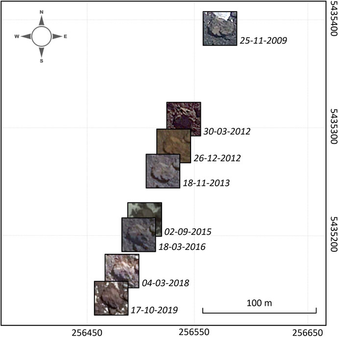
FIGURE 2. Tracking of a boulder located at the surface of the Verde glacier. Each dated square represent the same boulder on distinct cropped images from Google Earth. Red arrow on Figure 6A indicates the path of the present boulder. Coordinates in meters, universal transverse mercator (UTM) projection, zone 19, World Geodetic System (WGS84) datum.
Surface gradient was extracted from the SRTM DEM. However, this is made difficult due to the topography of DCGs being generally very coarse (Nicholson and Benn, 2012), and the SRTM showing random speckle noises (Stevenson et al., 2010), also referred as coherent multiplicative noises, that inherently exist in these products. Into QGIS, a low pass filter was thus initially applied, which is a common method to smooth SRTM DEMs (Wendi et al., 2016). Surface gradients were then grouped into four classes (0–2, 2–6, 6–10, and >10), as proposed by Reynolds (2000), and applied by Quincey et al. (2007) and Miles et al. (2017b) to analyse ponds and ice cliffs distribution. Root Mean Square Error (RMSE) was applied to compute the uncertainty of the two interpolation methods in comparison with the observations.
Results
Ponds and Ice Cliffs Inventory
Over the 2009–2019 period, a total of 151 ponds and 940 ice cliffs were identified (Table 2 and Figure 3). An example of mapped pond and ice cliff are shown on Figure 4. Both the ponds and the ice cliffs cover most of the tongue area, with highest density in the middle part. It is important to note that most of the ice cliffs located in the upper part of the tongue (Figure 3B) are associated with supraglacial channels.
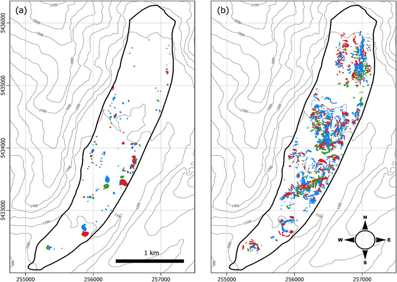
FIGURE 3. (A) Ponds and (B) ice cliffs observed over the 2009–2019 period on the debris-covered tongue of Verde glacier. Features are colour-coded in function of the period of the year they were mapped, blue corresponding to November 2009, December 2012 and November 2013; red to March 2012, March 2016, March 2018; and green to September 2015 and October 2019. Elevation data are based on SRTM DEM. Coordinates in meters, Universal Transverse Mercator (UTM) projection, zone 19, World Geodetic System (WGS84) datum.
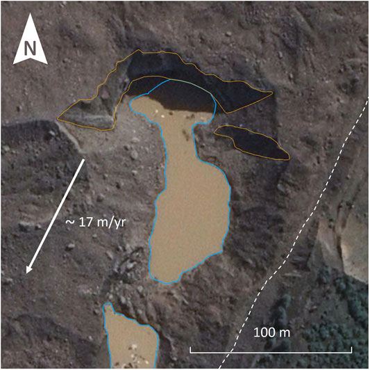
FIGURE 4. Outlines of mapped ponds (solid blue lines) and south-facing ice cliffs (solid orange lines), from march 4, 2018. White arrow indicates local mean surface velocity, extracted from spline interpolation surface. White dashed line shows the glacier outline.
The most extensive pond coverage was observed on March 30, 2012 (13,517 ± 649 m2), which represents 0.44 ± 0.02% of the debris-covered area. Regarding the maximum ice cliff cover (82,364 ± 9,355 m2), it occurs on November 25, 2009 and represents 2.70 ± 0.30% of the glacier tongue. Most of the ice cliffs (866 of 940) were not in contact with ponds at the moment of their mapping. High interannual variability is observed in both ponds and ice cliffs coverage (Figure 5).
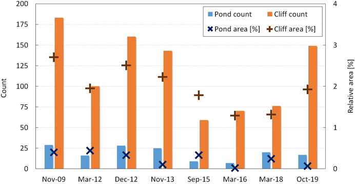
FIGURE 5. Observed ponds and ice cliffs number and area.
Surface Velocity
A total of 191 boulders were tracked at the glacier surface, allowing velocity measurements over most of the debris-covered tongue (Figure 6A). Some boulders show displacements not concordant with the flow line direction between two dates, which is likely due to topography effects and roll overs. Ten control points were tracked around the glacier tongue (Figure 6A), allowing to determine a maximum total displacement error of 0.3 m/yr along the flowline.
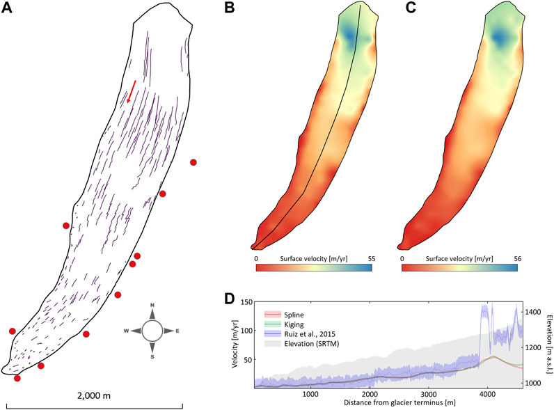
FIGURE 6. (A) Tracked boulders on the debris-covered tongue of Verde glacier between November 2009 and October 2019. The red arrow shows the location of the boulder of Figure 2. Red dots mark the location of control points outside glacier area (B, C) Interpolated surface velocity using spline and kriging interpolation methods, respectively.(D) Surface velocity profiles corresponding to the black line on (B). Shaded area correspond to error associated to the interpolated velocities. Blue line and light grey area show results from Ruiz et al. (2015) and the elevation along the same profile, respectively.
Both spline and kriging interpolations methods (Figures 6B,C) show statistically similar results (Table 3). Highest velocities are found in the upper part of the glacier tongue, just below the steep icefall, with a regular decrease towards the glacier terminus, which is almost stagnant. This is consistent with the surface slope becoming gradually shallower towards the snout (Figure 6D). Low velocities are also found on the margins of the glacier. Our results are concordant with findings from Ruiz et al. (2015) which shown that higher velocities are associated with the ice fall and found almost stagnant conditions in the lower reach and lateral margins of the debris-covered tongue (Figure 6D). Otherwise, some discrepancies appear in the upper limits of the covered-tongue, likely associated with a lack of mapped boulders in this area of the glacier and a greatest uncertainty while applying interpolation techniques.

TABLE 3. Main statistical characteristics of the interpolated velocity results.
Ice Cliff Backwasting
Eleven ice cliffs were identified to persist over at least two scenes of the period of interest. Retreat varies from a few meters to a maximum distance of 201 m between November 2009 and October 2, 2019 for a ∼200 m wide ice cliff (Figure 7B). After correction for local surface velocity, the highest backwasting rate was assessed to 24 m/yr for a south-facing ice cliff (third arrow from the north on Figure 7), while the measured retreat was about 9 m/yr.
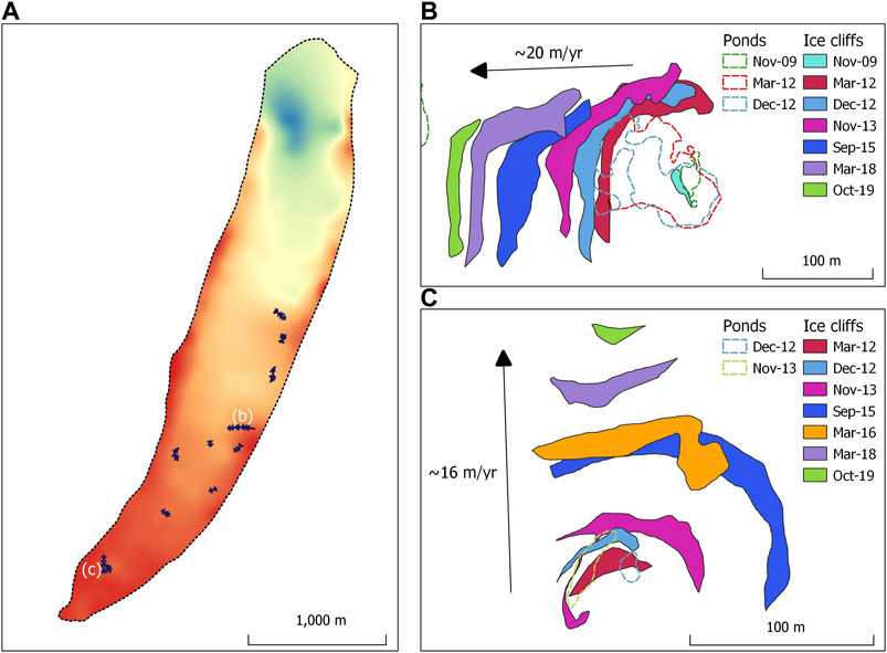
FIGURE 7. (A) Direction and length of retreat of 11 ice cliffs on the debris-covered tongue of Verde glacier. Colormap corresponds to the spline interpolation of surface velocity of Figure 6B. (B) and (C) refer to the right panels showing detailed time-lapse retreat of two selected ice cliffs and the associated ponds.
Discussion
Ponds and Ice Cliff Distribution and Formation
Although supraglacial ponds and ice cliffs are observed across the whole elevation range, their distribution is uneven over the tongue (Figure 3). Four main clusters can be identified, from North to South, in particular when describing the ice cliffs distribution (Figure 3B). The first cluster counts few ponds and two channels of numerous ice cliffs parallel to the flowline. The formation of these ice cliffs seems to be associated with supraglacial channels visible on the upper part of the debris-covered tongue. The second and the third clusters show the largest populations of ponds and ice cliffs. A clear gap, showing no features, is visible between the first and the second clusters, which we attributed to a huge quantity of debris deposited on the tongue by a landslide or rock avalanche originated on the western flanks of the valley (Figure 1). A smallest gap is observed between the second and the third cluster, likely associated with a former landslide or rock avalanche, forming visible arched ridges on the glacier surface. These thick deposits of debris appear to be inhibiting the formation of supraglacial ponds and ice cliffs at the glacier surface. Finally, the fourth cluster, located near the front, shows smaller density of ponds and ice cliffs, whereas reduced surface velocity and gentle slopes would be adequate for their formation (see Figure 3). We attributed this small amount of feature to a significant debris thickness, highlighted by the presence of trees and vegetation on the glacier surface (Figure 1). The lowest ponds and ice cliffs numbers in the areas with thicker debris layers is concordant with results from Steiner et al. (2019) in the Langtang catchment (Himalaya), who observed few features near the front, where the debris layer is the thickest. The absence of ponds and cliffs in areas of thick debris is likely due to suppression of ablation, as the insulation threshold might be exceeded.
All mapped ponds take place on the tongue with gradient below 10 (Figure 8). Above this threshold, all the available meltwater is able to drain away, as previously reported by (Reynolds, 2000) on DCGs in Bhutan. Specifically, 14, 74 and 12% of the ponds were observed on slopes <2°, between 2–6 and between 6–10, respectively. These distributions are concordant with observations made on DCGs in Himalaya (Liu et al., 2015; Chand and Watanabe, 2019).
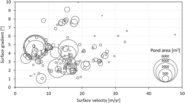
FIGURE 8. Pond area as a function of surface gradient and interpolated velocity (derived form the spline method). Pond area is proportional to circles size.
The ice cliffs distribution shows a similar pattern with less than 1% observed on areas with gradient above 10, while 10, 73 and 16% of the mapped cliffs are located on slopes <2°, between 2–6 and between 6–10, respectively. These similar distributions of ponds and ice cliffs with respect to gradient could signify their formations are associated processes. Indeed, despite the fact that only 70 of 907 ice cliffs were in contact with a pond at the moment of their mapping, we observed that most of the backwasting ice cliffs (Table 4) are in contact with a pond at the initial stages of their formation (Figures 7B,C). Afterwards, the cliffs lose contact as they retreat and the ponds are either drained or filled with debris.
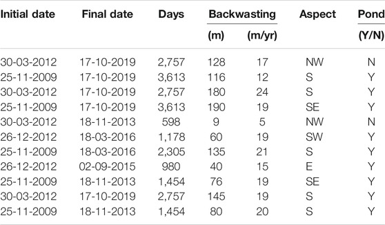
TABLE 4. Persistent and backwasting ice cliffs on Verde glacier, listed from north to south. The ‘Pond’ column indicates the presence (Y) or not (N) of a coalescent pond at any stage of the backwasting process.
The distribution of ponds with respect to their surface area is strongly controlled by both surface gradient and surface velocity (Figure 8). Large ponds (>1,000 m2) only develop on glacier surface of relatively low velocity (<17 m/yr) and low gradient (<6). This results in large ponds being constrained to the lower-half and the margins of the tongue (Figure 3A).
Regarding the distribution of ice cliffs with respect to their area, no clear influence of surface velocity nor surface gradient was observed (Figure 9). Nevertheless, it appears that large ice cliffs only develop where surface velocity is low (Figure 9A).
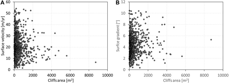
FIGURE 9. Cliff area as a function of (A) surface velocity, derived from the spline interpolation, and (B) surface gradient, extracted from SRTM.
The observed high variability in ponds and ice cliff distribution and their interannual evolution seems to highlight a very dynamic behaviour of Verde glacier, which is concordant with observed high surface velocity. These observations tends to demonstrate that the supraglacial ponds do connect and disconnect with the englacial conduits as crevasses open and close, respectively.
Seasonality
No long-term trend in ponds and ice cliffs count or covered area was detected between 2009 and 2019. On the other hand, and based on the available data, we observed a seasonal signal in the number of supraglacial ponds and in the number and area of ice cliff mapped through the year (Table 2; Figure 5). We found a maximum of supraglacial ponds and ice cliffs during spring and at the beginning of summer (November 2009, December 2012, November 2013, October 2019), and a minimum of ponds and ice cliffs, at the end of summer (March 2012, March 2016, March 2018), and at the end of winter (September 2015). We suggest the number of ponds and number and area of ice-cliff might be related to the evolution of the hydrological network through the year, as previously proposed in other studies (Reynolds, 2000; Sakai et al., 2000). At the beginning of the ablation period (spring and beginning of summer), the hydrological network is not well connected yet, so meltwater accumulated into depressions and form supgraglacial ponds. This early pond formation initiates the exposure of associated ice cliffs. During the ablation season, the crevasses and englacial conduits open and enhance connectivity. Similar cycles have been observed in the Eastern Himalaya and Karakoram, with an increase in ponds number at the beginning of spring (April) and a sharp decrease in June-July (Narama et al., 2017). Authors attributed the increase to inflow of meltwater from snow and ice, and the later decrease to a enhanced connectivity to the englacial drainage network. The earlier part of the cycle was also observed in High Mountain Asia during the pre-monsoon season, and related to the observed reduction of the snow cover (Miles et al., 2017b; Chand and Watanabe, 2019).
Finally, during the beginning of the accumulation season (winter), there is no meltwater at the surface to fill the ponds. This small amount of ponds and their reduced cover in winter are concordant with results from the Everest region (Chand and Watanabe, 2019).
The smallest amount of ice cliffs at the end of summer might also be related to their fast-vanishing behaviour, as few of them have been observed to persist year to year which could also explains that no seasonality was observed regarding the ponds area.
Characteristics of Backwasting Ice Cliffs
Most of the persistent and backwasting ice cliffs were found to be south-facing (Table 4), which is consistent with results from Sakai et al. (2002) and Buri and Pellicciotti (2018), who found that persistent ice cliffs are mostly north-facing in the northern hemisphere. In all cases, persistent ice cliffs appear to be pole-facing. In contrast, the sun-facing ice cliffs do not have time to extent spatially, and do not survive the ablation season, as they receive the highest amount of radiations. They are thought to not contribute significantly to annual mass balance (Buri and Pellicciotti, 2018). According to Sakai et al. (2002), the difference in stability between the pole-facing and the sun-facing ice cliffs is caused by a difference in incoming radiations. Pole-facing cliffs receive mostly long-wave radiation from the surrounding debris cover, which reaches the lower portion more than the upper portion. This results in the ice cliff being steep enough to not be covered by debris and persist over time. On the other hand, sun-facing cliffs are exposed to direct and more intense short-wave radiation, which affect mainly their upper portion. These cliffs have thus shallower slope and are more likely to get covered by debris.
The growth and demise of a persistent south-facing ice cliff on glacier Verde is illustrated on Figure 7C. This south-facing ice cliff initially emerges as a concave feature in contact with a pond. The ice cliff then grows spatially and reach a maximal extent, before it tails off as a convex feature. In the later stages, there is no apparent pond adjacent to the persistent ice cliffs.
Conclusion
We have compiled a complete inventory of supraglacial ponds and ice cliffs of the debris-covered tongue of Verde glacier, in the Chilean Northern Patagonian Andes. The inventory was based on Google Earth historical imagery covering the 2009–2019 period. Coverage ranges from 0.02 to 0.44% for ponds, and from 0.51 to 2.70% for ice cliffs.
Supraglacial ponds and ice cliffs are present at every elevation range of the debris-covered tongue. Ponds distribution is controlled by surface characteristics, with large features only occurring on areas of reduced velocity and low gradient. Ice cliffs distribution is less clear and appears to be slightly controlled by surface velocity. Debris thickness appears to also play a role in the presence or not of ponds and cliffs, as areas of thicker debris covers exhibit none of the two features. Based on available data, supraglacial ponds count and ice-cliff count and area exhibit a seasonal signal, with a maximum during the beginning of the ablation season and a minimum at the end of the ablation season and through the accumulation seasons. We attribute this seasonality to the opening and closure of the hydrological network through the year. Finally, we identified eleven persistent ice cliffs, most of them south-facing (or pole-facing). Ice cliff backwasting up to 200 m was observed, which highlights that ablation processes take place on the glacier surface, contrasting with the stagnant terminus.
Further researches need to be conducted to address the role of supraglacial ponds and ice cliffs on glacier mass balance, as well as their impact on the hydrological regime of DCGs. A continuous in-situ monitoring of ponds and ice cliff evolution could give insights into their interannual evolution, as well as the frequency and velocity of drainage and filling.
Data Availability Statement
The raw data supporting the conclusions of this article will be made available by the authors, without undue reservation.
Author Contributions
TL gathered and prepared all data, performed all processing and calculations, and made all figures and tables. TL and LR contributed to the discussion of results, and shared the writing of the paper.
Funding
The Centro de Estudios Cientificos (CECs) is co-funded by the base Finance program of ANID/PIA APOYO CCTE AFB170003. LR acknowledges supports from Ministerio de Ambiente y Desarrollo Sustentable de Argentina (Inventario Nacional de Glaciares), Agencia de Promocion Cientfica (projects PICT 2010-1,438; PICT 2014-1794) and CONICET.
Conflict of Interest
The authors declare that the research was conducted in the absence of any commercial or financial relationships that could be construed as a potential conflict of interest.
References
Alifu, H., Johnson, B. A., and Tateishi, R. (2016a). Delineation of Debris-Covered Glaciers Based on a Combination of Geomorphometric Parameters and a TIR/NIR/SWIR Band Ratio. IEEE J. Sel. Top. Appl. Earth Observations Remote Sensing 9 (2), 781–792. doi:10.1109/jstars.2015.2500906
Alifu, H., Tateishi, R., Alsaaideh, B., and Gharechelou, S. (2016b). Multi-criteria Technique for Mapping of Debris-Covered and Clean-Ice Glaciers in the Shaksgam valley Using Landsat TM and ASTER GDEM. J. Mountain Sci. 13 (4), 703–714.
Anderson, R. S., Anderson, L. S., Armstrong, W. H., Rossi, M. W., and Crump, S. E. (2018). Glaciation of alpine Valleys: The Glacier - Debris-Covered Glacier - Rock Glacier Continuum. Geomorphology 311, 127–142. doi:10.1016/j.geomorph.2018.03.015
Aravena, J.-C., and Luckman, B. H. (2009). Spatio-temporal Rainfall Patterns in Southern South America. Int. J. Climatol. 29, 2106–2120. doi:10.1002/joc.1761
Ayala, A., Pellicciotti, F., MacDonell, S., McPhee, J., Vivero, S., Campos, C., et al. (2016). Modelling the Hydrological Response of Debris-free and Debris-Covered Glaciers to Present Climatic Conditions in the Semiarid Andes of central Chile. Hydrol. Process. 30 (22), 4036–4058. doi:10.1002/hyp.10971
Barcaza, G., Nussbaumer, S. U., Tapia, G., Valdés, J., García, J. L., Videla, Y., et al. (2017). Glacier Inventory and Recent Glacier Variations in the Andes of Chile, South America. Ann. Glaciology 58 (75), 166–180. doi:10.1017/aog.2017.28
Benn, D. I., Bolch, T., Hands, K., Gulley, J., Luckman, A., Nicholson, L. I., et al. (2012). Response of Debris-Covered Glaciers in the Mount Everest Region to Recent Warming, and Implications for Outburst Flood Hazards. Earth-Science Rev. 114 (1-2), 156–174. doi:10.1016/j.earscirev.2012.03.008
Bhushan, S., Syed, T. H., Arendt, A. A., Kulkarni, A. V., and Sinha, D. (2018). Assessing Controls on Mass Budget and Surface Velocity Variations of Glaciers in Western Himalaya. Sci. Rep. 8 (1), 8885–8911. doi:10.1038/s41598-018-27014-y
Bisset, R. R., Dehecq, A., Goldberg, D. N., Huss, M., Bingham, R. G., and Gourmelen, N. (2020). Reversed Surface-Mass-Balance Gradients on Himalayan Debris-Covered Glaciers Inferred from Remote Sensing. Remote Sensing 12 (10). doi:10.3390/rs12101563
Brock, B., Rivera, A., Casassa, G., Bown, F., and Acuña, C. (2007). The Surface Energy Balance of an Active Ice-Covered Volcano: Villarrica Volcano, Southern Chile. Ann. Glaciol. 45 (1), 104–114. doi:10.3189/172756407782282372
Brun, F., Wagnon, P., Berthier, E., Shea, J. M., Immerzeel, W. W., Kraaijenbrink, P. D. A., et al. (2018). Ice Cliff Contribution to the Tongue-wide Ablation of Changri Nup Glacier, Nepal, central Himalaya. The Cryosphere 12 (11), 3439–3457. doi:10.5194/tc-12-3439-2018
Burger, F., Ayala, A., Farias, D., Shaw, T. E., MacDonell, S., Brock, B., et al. (2019). Interannual Variability in Glacier Contribution to Runoff from a High‐elevation Andean Catchment: Understanding the Role of Debris Cover in Glacier Hydrology. Hydrological Process. 33 (2), 214–229. doi:10.1002/hyp.13354
Buri, P., and Pellicciotti, F. (2018). Aspect Controls the Survival of Ice Cliffs on Debris-Covered Glaciers. Proc. Natl. Acad. Sci. USA 115 (17), 4369–4374. doi:10.1073/pnas.1713892115
Carrasco, J. F., Casassa, G., and Quintana, J. (2005). Changes of the 0°C isotherm and the equilibrium line altitude in central Chile during the last quarter of the 20th century/Changements de l'isotherme 0°C et de la ligne d'équilibre des neiges dans le Chili central durant le dernier quart du 20ème siècle. Hydrological Sci. J. 50 (6), 933–948. doi:10.1623/hysj.2005.50.6.933
Casassa, G., Rodríguez, J. L., and Loriaux, T. (2014). A New Glacier Inventory for the Southern Patagonia Icefield and Areal Changes 1986-2000. In Global Land Ice Measurements from Space, pages 639–660. doi:10.1007/978-3-540-79818-7_27
Chand, M. B., and Watanabe, T. (2019). Development of Supraglacial Ponds in the Everest Region, Nepal, between 1989 and 2018. Remote Sensing 11 (9). doi:10.3390/rs11091058
Charbonneau, A. A., and Smith, D. J. (2018). An Inventory of Rock Glaciers in the central British Columbia Coast Mountains, Canada, from High Resolution Google Earth Imagery. Arctic, Antarctic, Alpine Res. 50 (1). doi:10.1080/15230430.2018.1489026
Chikita, K., Jha, J., and Yamada, T. (1998). The basin Expansion Mechanism of a Supraglacial lake in the Nepal Himalaya. J. Hokkaido Univ. Fac. Sci. Ser. VII: Geophys. 11 (2), 501–521.
Collier, E., Maussion, F., Nicholson, L. I., Mölg, T., Immerzeel, W. W., and Bush, A. B. G. (2015). Impact of Debris Cover on Glacier Ablation and Atmosphere-Glacier Feedbacks in the Karakoram. The Cryosphere 9 (4), 1617–1632. doi:10.5194/tc-9-1617-2015
Condom, T., Coudrain, A., Sicart, J. E., and Théry, S. (2007). Computation of the Space and Time Evolution of Equilibrium-Line Altitudes on Andean Glaciers (10N-55S). Glob. Planet. Change 59 (1-4), 189–202. doi:10.1016/j.gloplacha.2006.11.021
Deline, P. (2005). Change in Surface Debris Cover on Mont Blanc Massif Glaciers after the'Little Ice Age' Termination. The Holocene 15, 302–309. doi:10.1191/0959683605hl809rr
Ferri, L., Dussaillant, I., Zalazar, L., Masiokas, M. H., Ruiz, L., Pitte, P., et al. (2020). Ice Mass Loss in the Central Andes of Argentina between 2000 and 2018 Derived from a New Glacier Inventory and Satellite Stereo-Imagery. Front. Earth Sci. 8 (December), 1–16. doi:10.3389/feart.2020.530997
Fyffe, C. L., Brock, B. W., Kirkbride, M. P., Black, A. R., Smiraglia, C., and Diolaiuti, G. (2019). The Impact of Supraglacial Debris on Proglacial Runoff and Water Chemistry. J. Hydrol. 576, 41–57. doi:10.1016/j.jhydrol.2019.06.023
Fyffe, C. L., Brock, B. W., Kirkbride, M. P., Mair, D. W. F., and Diotri, F. (2012). The Hydrology of a Debris-Covered Glacier, the Miage Glacier, Italy. BHS Eleventh National Symposium, Hydrology For a Changing World. Dundee ((January).
Garreaud, R. D., Vuille, M., Compagnucci, R., and Marengo, J. (2009). Present-day South American Climate. Palaeogeogr. Palaeoclimatol. Palaeoecol. 281 (3-4), 180–195. doi:10.1016/j.palaeo.2007.10.032
Hagg, W., Mayer, C., Lambrecht, A., and Helm, A. (2008). Sub‐debris Melt Rates on Southern Inylchek Glacier, central Tian Shan. Geografiska Annaler: Ser. A, Phys. Geogr. 90 (1), 55–63. doi:10.1111/j.1468-0459.2008.00333.x
Immerzeel, W. W., Kraaijenbrink, P. D. A., Shea, J. M., Shrestha, A. B., Pellicciotti, F., Bierkens, M. F. P., et al. (2014). High-resolution Monitoring of Himalayan Glacier Dynamics Using Unmanned Aerial Vehicles. Remote Sensing Environ. 150, 93–103. doi:10.1016/j.rse.2014.04.025
Immerzeel, W. W., Lutz, A. F., Andrade, M., Bahl, A., Biemans, H., Bolch, T., et al. (2020). Importance and Vulnerability of the World's Water Towers. Nature 577 (7790), 364–369. doi:10.1038/s41586-019-1822-y
Irvine-Fynn, T. D. L., Porter, P. R., Rowan, A. V., Quincey, D. J., Gibson, M. J., Bridge, J. W., et al. (2017). Supraglacial Ponds Regulate Runoff from Himalayan Debris-Covered Glaciers. Geophys. Res. Lett. 44 (23), 11894–11094. doi:10.1002/2017gl075398
Iwata, S., Watanabe, O., and Fushimi, H. (1980). Surface Morphology in the Ablation Area of the Khumbu Glacier. J. Jpn. Soc. Snow Ice 41 (Special), 9–17. doi:10.5331/seppyo.41.special_9
Janke, J. R., Bellisario, A. C., and Ferrando, F. A. (2015). Classification of Debris-Covered Glaciers and Rock Glaciers in the Andes of central Chile. Geomorphology 241, 98–121. doi:10.1016/j.geomorph.2015.03.034
Jones, D. B., Harrison, S., Anderson, K., Selley, H. L., Wood, J. L., and Betts, R. A. (2018). The Distribution and Hydrological Significance of Rock Glaciers in the Nepalese Himalaya. Glob. Planet. Change 160 (November), 123–142. doi:10.1016/j.gloplacha.2017.11.005
Kirkbride, M. P. (1993). The Temporal Significance of Transitions from Melting to Calving Termini at Glaciers in the central Southern Alps of New Zealand. The Holocene 3 (3), 232–240. doi:10.1177/095968369300300305
Knight, J., Harrison, S., and Jones, D. B. (2019). Rock Glaciers and the Geomorphological Evolution of Deglacierizing Mountains. Geomorphology 324, 14–24. doi:10.1016/j.geomorph.2018.09.020
Liu, Q., Mayer, C., and Liu, S. (2015). Distribution and Interannual Variability of Supraglacial Lakes on Debris-Covered Glaciers in the Khan Tengri-Tumor Mountains, Central Asia. Environ. Res. Lett. 10 (1).
Lliboutry, L. (1998). “Glacier of Chile and Argentina,” in Glaciers Of South America, Pages 109–206. Editors R. S. Williams, and J. G. Ferrigno edition (Washington, isgs profe: USGS).
Maurer, J. M., Rupper, S. B., and Schaefer, J. M. (2016). Quantifying Ice Loss in the Eastern Himalayas since 1974 Using Declassified Spy Satellite Imagery. Cryosphere Discuss. 10, 2203–2215. doi:10.5194/tc-10-2203-2016
Miles, E. S., Willis, I., Buri, P., Steiner, J. F., Arnold, N. S., and Pellicciotti, F. (2018). Surface Pond Energy Absorption across Four Himalayan Glaciers Accounts for 1/8 of Total Catchment Ice Loss. Geophys. Res. Lett. 45 (1910), 10464–10473. doi:10.1029/2018GL079678
Miles, E. S., Steiner, J., Willis, I., Buri, P., Immerzeel, W. W., Chesnokova, A., et al. (2017a). Pond Dynamics and Supraglacial-Englacial Connectivity on Debris-Covered Lirung Glacier, Nepal. Front. Earth Sci. 5 (September), 1–19. doi:10.3389/feart.2017.00069
Miles, E. S., Willis, I. C., Arnold, N. S., Steiner, J., and Pellicciotti, F. (2017b). Spatial, Seasonal and Interannual Variability of Supraglacial Ponds in the Langtang Valley of Nepal, 1999-2013. J. Glaciol. 63 (237), 88–105. doi:10.1017/jog.2016.120
Miles, K. E., Hubbard, B., Irvine-Fynn, T. D. L., Miles, E. S., Quincey, D. J., and Rowan, A. V. (2020). Hydrology of Debris-Covered Glaciers in High Mountain Asia. Earth-Science Rev. 207 (June), 103212. doi:10.1016/j.earscirev.2020.103212
Miles, K. E., Hubbard, B., Quincey, D. J., Miles, E. S., Irvine-Fynn, T. D. L., and Rowan, A. V. (2019). Surface and Subsurface Hydrology of Debris-Covered Khumbu Glacier, Nepal, Revealed by Dye Tracing. Earth Planet. Sci. Lett. 513, 176–186. doi:10.1016/j.epsl.2019.02.020
Monnier, S., and Kinnard, C. (2017). Pluri-decadal (1955-2014) Evolution of Glacier-Rock Glacier Transitional Landforms in the central Andes of Chile (30-33° S). Earth Surf. Dynam. 5 (3), 493–509. doi:10.5194/esurf-5-493-2017
Monnier, S., and Kinnard, C. (2015). Reconsidering the Glacier to Rock Glacier Transformation Problem: New Insights from the central Andes of Chile. Geomorphology 238, 47–55. doi:10.1016/j.geomorph.2015.02.025
Nagai, H., Fujita, K., Sakai, A., Nuimura, T., and Tadono, T. (2016). Comparison of Multiple Glacier Inventories with a New Inventory Derived from High-Resolution ALOS Imagery in the Bhutan Himalaya. The Cryosphere 10 (1), 65–85. doi:10.5194/tc-10-65-2016
Narama, C., Daiyrov, M., Tadono, T., Yamamoto, M., Kääb, A., Morita, R., et al. (2017). Seasonal Drainage of Supraglacial Lakes on Debris-Covered Glaciers in the Tien Shan Mountains, Central Asia. Geomorphology 286, 133–142. doi:10.1016/j.geomorph.2017.03.002
Nicholson, L., and Benn, D. I. (2012). Properties of Natural Supraglacial Debris in Relation to Modelling Sub-debris Ice Ablation. Earth Surf. Process. Landforms 38 (5), 490–501. doi:10.1002/esp.3299
Pandey, P. (2019). Inventory of Rock Glaciers in Himachal Himalaya, India Using High-Resolution Google Earth Imagery. Geomorphology 340, 103–115. doi:10.1016/j.geomorph.2019.05.001
Paul, F., and Mölg, N. (2014). Hasty Retreat of Glaciers in Northern Patagonia from 1985 to 2011. J. Glaciol. 60 (224), 1033–1043. doi:10.3189/2014jog14j104
Pellicciotti, F., Stephan, C., Miles, E., Herreid, S., Immerzeel, W. W., and Bolch, T. (2015). Mass-balance Changes of the Debris-Covered Glaciers in the Langtang Himal, Nepal, from 1974 to 1999. J. Glaciol. 61 (226), 373–386. doi:10.3189/2015jog13j237
Quincey, D. J., Richardson, S. D., Luckman, A., Lucas, R. M., Reynolds, J. M., Hambrey, M. J., et al. (2007). Early Recognition of Glacial lake Hazards in the Himalaya Using Remote Sensing Datasets. Glob. Planet. Change 56 (1-2), 137–152. doi:10.1016/j.gloplacha.2006.07.013
Rangecroft, S., Harrison, S., Anderson, K., Magrath, J., Castel, A. P., and Pacheco, P. (2014). A First Rock Glacier Inventory for the Bolivian Andes. Permafrost Periglac. Process. 25 (4), 333–343. doi:10.1002/ppp.1816
Reid, T. D., and Brock, B. W. (2014). Assessing Ice-Cliff Backwasting and its Contribution to Total Ablation of Debris-Covered Miage Glacier, Mont Blanc Massif, Italy. J. Glaciol. 60 (219), 3–13. doi:10.3189/2014jog13j045
Reinthaler, J., Paul, F., Granados, H. D., Rivera, A., and Huggel, C. (2019). Area Changes of Glaciers on Active Volcanoes in Latin America between 1986 and 2015 Observed from Multi-Temporal Satellite Imagery. J. Glaciol. 65, 542–556. doi:10.1017/jog.2019.30
Reynolds, J. M. (2000). On the Formation of Supraglacial Lakes on Debris-Covered Glaciers. Seattle: IAHS-AISH Publication, 153–161.
Röhl, K. (2008). Characteristics and Evolution of Supraglacial Ponds on Debris-Covered Tasman Glacier, New Zealand. J. Glaciol. 54 (188), 867–880. doi:10.3189/002214308787779861
Ruiz, L., Berthier, E., Masiokas, M., Pitte, P., and Villalba, R. (2015). First Surface Velocity Maps for Glaciers of Monte Tronador, North Patagonian Andes, Derived from Sequential Pléiades Satellite Images. J. Glaciol. 61 (229), 908–922. doi:10.3189/2015jog14j134
Ruiz, L., Berthier, E., Viale, M., Pitte, P., and Masiokas, M. H. (2017). Recent Geodetic Mass Balance of Monte Tronador Glaciers, Northern Patagonian Andes. The Cryosphere 11 (1), 619–634. doi:10.5194/tc-11-619-2017
Sakai, A., and Fujita, K. (2010). Formation Conditions of Supraglacial Lakes on Debris- Covered Glaciers in the Himalaya. J. Glaciology 56 (195), 231–326. doi:10.3189/002214310791190785
Sakai, A., Nakawo, M., and Fujita, K. (2002). Distribution Characteristics and Energy Balance of Ice Cliffs on Debris-Covered Glaciers, Nepal Himalaya. Arctic, Antarctic, Alpine Res. 34 (1), 12–19. doi:10.1080/15230430.2002.12003463
Sakai, A., Takeuchi, N., Fujita, K., and Nakawo, M. (2000). Seattle: IAHS-AISH Publication, 119–130.Role of Supraglacial Ponds in the Ablation Process of a Debris-Covered Glacier in the Nepal Himalayas264
Salerno, F., Thakuri, S., D’Agata, C., Smiraglia, C., Manfredi, E. C., Viviano, G., et al. (2012). Glacial lake Distribution in the Mount Everest Region: Uncertainty of Measurement and Conditions of Formation. Glob. Planet. Change 92-93, 30–39. doi:10.1016/j.gloplacha.2012.04.001
Schmid, M.-O., Baral, P., Gruber, S., Shahi, S., Shrestha, T., Stumm, D., et al. (2015). Assessment of Permafrost Distribution Maps in the Hindu Kush Himalayan Region Using Rock Glaciers Mapped in Google Earth. The Cryosphere 9 (6), 2089–2099. doi:10.5194/tc-9-2089-2015
Steiner, J. F., Buri, P., Miles, E. S., Ragettli, S., and Pellicciotti, F. (2019). Supraglacial Ice Cliffs and Ponds on Debris-Covered Glaciers: Spatio-Temporal Distribution and Characteristics. J. Glaciol. 65 (252), 617–632. doi:10.1017/jog.2019.40
Steiner, J. F., Pellicciotti, F., Buri, P., Miles, E. S., Immerzeel, W. W., and Reid, T. D. (2015). Modelling Ice-Cliff Backwasting on a Debris-Covered Glacier in the Nepalese Himalaya. J. Glaciol. 61 (229), 889–907. doi:10.3189/2015jog14j194
Stevenson, J. A., Sun, X., and Mitchell, N. C. (2010). Despeckling SRTM and Other Topographic Data with a Denoising Algorithm. Geomorphology 114 (3), 238–252. doi:10.1016/j.geomorph.2009.07.006
Stokes, C. R., Popovnin, V., Aleynikov, A., Gurney, S. D., and Shahgedanova, M. (2007). Recent Glacier Retreat in the Caucasus Mountains, Russia, and Associated Increase in Supraglacial Debris Cover and Supra-/proglacial lake Development. Ann. Glaciol. 46 (5642 m), 195–203. doi:10.3189/172756407782871468
Thakuri, S., Salerno, F., Smiraglia, C., Bolch, T., D'Agata, C., Viviano, G., et al. (2014). Tracing Glacier Changes since the 1960s on the South Slope of Mt. Everest (central Southern Himalaya) Using Optical Satellite Imagery. The Cryosphere 8 (4), 1297–1315. doi:10.5194/tc-8-1297-2014
Thompson, S., Benn, D. I., Mertes, J., and Luckman, A. (2016). Stagnation and Mass Loss on a Himalayan Debris-Covered Glacier: Processes, Patterns and Rates. J. Glaciol. 62 (233), 467–485. doi:10.1017/jog.2016.37
Tielidze, L. G., Bolch, T., Wheate, R. D., Kutuzov, S. S., Lavrentiev, I. I., and Zemp, M. (2020). Supra-glacial Debris Cover Changes in the Greater Caucasus from 1986 to 2014. The Cryosphere 14 (2), 585–598. doi:10.5194/tc-14-585-2020
Viale, M., Bianchi, E., Cara, L., Ruiz, L., Villalba, R., Pitte, P., et al. (2019). Contrasting Climates at Both Sides of the Andes in Argentina and Chile. Front. Environ. Sci. 7 (May), 1–15. doi:10.3389/fenvs.2019.00069
Viale, M., and Garreaud, R. (2015). Orographic Effects of the Subtropical and Extratropical Andes on Upwind Precipitating Clouds. J. Geophys. Res. Atmospheres 120, 1–13. doi:10.1002/2014jd023014
Watson, C. S., King, O., Miles, E. S., and Quincey, D. J. (2018a). Optimising NDWI Supraglacial Pond Classification on Himalayan Debris-Covered Glaciers. Remote Sensing Environ. 217 (August), 414–425. doi:10.1016/j.rse.2018.08.020
Watson, C. S., Quincey, D. J., Carrivick, J. L., Smith, M. W., Rowan, A. V., and Richardson, R. (2018b). Heterogeneous Water Storage and thermal Regime of Supraglacial Ponds on Debris-Covered Glaciers. Earth Surf. Process. Landforms 43 (1), 229–241. doi:10.1002/esp.4236
Wendi, D., Liong, S.-Y., Sun, Y., and Doan, C. D. (2016). An Innovative Approach to Improve SRTM DEM Using Multispectral Imagery and Artificial Neural Network. J. Adv. Model. Earth Syst. 8, 691–702. doi:10.1002/2015ms000536
Wigmore, O., and Mark, B. (2017). Monitoring Tropical Debris Covered Glacier Dynamics from High Resolution Unmanned Aerial Vehicle Photogrammetry. Cordillera Blanca, Peru: The Cryosphere 11, 2463–2480. doi:10.5194/tc-11-2463-2017
Wilson, R., Glasser, N. F., Reynolds, J. M., Harrison, S., Anacona, P. I., Schaefer, M., et al. (2018). Glacial Lakes of the Central and Patagonian Andes. Glob. Planet. Change 162, 275–291. doi:10.1016/j.gloplacha.2018.01.004
Zalazar, L., Ferri, L., Castro, M., Gargantini, H., Gimenez, M., Pitte, P., et al. (2020). Spatial Distribution and Characteristics of Andean Ice Masses in Argentina: Results from the First National Glacier Inventory. J. Glaciol. 66 (260), 938–949. doi:10.1017/jog.2020.55
Keywords: debris-covered glacier, chile, supraglacial ponds, ice cliffs, glacier velocity, Southern Andes
Citation: Loriaux T and Ruiz L (2021) Spatio-Temporal Distribution of Supra-Glacial Ponds and Ice Cliffs on Verde Glacier, Chile. Front. Earth Sci. 9:681071. doi: 10.3389/feart.2021.681071
Received: 15 March 2021; Accepted: 20 May 2021;
Published: 08 June 2021.
Edited by:
Aparna Shukla, Ministry of Earth Sciences, IndiaReviewed by:
Purushottam Kumar Garg, Wadia Institute of Himalayan Geology, IndiaBenjamin Brock, Northumbria University, United Kingdom
Copyright © 2021 Loriaux and Ruiz. This is an open-access article distributed under the terms of the Creative Commons Attribution License (CC BY). The use, distribution or reproduction in other forums is permitted, provided the original author(s) and the copyright owner(s) are credited and that the original publication in this journal is cited, in accordance with accepted academic practice. No use, distribution or reproduction is permitted which does not comply with these terms.
*Correspondence: Thomas Loriaux, dGhvbWFzQGNlY3MuY2w=