 Jae-Ho Lee
 You-Soon Chang
- Department of Earth Science Education, Kongju National University, Kongju, South Korea
In this study, we developed a new high-resolution regional climatology (0.1° by 0.1° by 19 levels) in the East/Japan Sea. National Centers for Environmental Information and Korea Oceanic Data Center already released the regional climatology of East Asian seas including the East/Japan Sea with 0.1° by 0.1° resolution. It provides a reliable temperature and salinity structure compared to previous 1° or 0.25° climatologies. However, this study found an abnormal meridional temperature gradient problem when calculating geostrophic currents based on this new climatology. Geostrophic currents show a strong repetitive eastward flow along the 1° latitudinal band especially in the East/Japan Sea, which corresponds with abnormal meridional temperature gradients at the same areas. This problem could be related to the objective analysis procedure generating the high-resolution climatology. Here, we reproduced a high-resolution climatology without the abnormal meridional temperature gradient problem by using the optimal interpolation method. Results show that the meridional gradient problem can partly be attributed to both the use of the World Ocean Atlas background field on the 1° grid, and the spatial distribution of World Ocean database observation data; however, these are not the primary causes. We corrected the abnormal temperature gradient by increasing the meridional decorrelation length scale without losing the meso-scale feature in the East/Japan Sea, as shown by the wavelet analysis. Improvement of the new gridded field is also validated by using serial hydrographic data and the altimetry-derived surface current product.
Introduction
The World Ocean Atlas (WOA) has been developed by the National Centers for Environmental Information (NCEI) to describe the three-dimensional temperature and salinity structures of the world ocean. It has served as initial and boundary conditions of ocean circulation models and validated ocean remote sensing data. The original WOA produced in 1982 (Levitus, 1982) was continuously updated through 1994 (NOAA, 1994), 1998 (NOAA, 1998), 2001 (Levitus, 2002; hereafter WOA01), 2005 (Levitus, 2006; hereafter WOA05), 2009 (Levitus, 2009; hereafter WOA09), 2013 (Levitus, 2013; hereafter WOA13), and 2018 (Boyer et al., 2018; hereafter WOA18) as the latest observations became available [https://www.ncei.noaa.gov/products/world-ocean-atlas]. However, WOAs except for recent versions (WOA13 and WOA18) have been produced with a spatial resolution of 1° × 1° on 33 vertical standard depth levels, hence they depict only the general temperature and salinity structure of large-scale in the global ocean.
Boyer and Levitus (1997) first improved the spatial resolution of ocean climatology with 0.25°; however, noise problems associated with spare data coverage were identified by a later study (Chang and Chao, 2000). By employing an additional smoothing scale, Boyer et al. (2005) developed a reliable 0.25° climatology; NCEI climatology is frequently updated and continues to be widely used. Gridded data from a Generalized Digital Environmental Model (GDEM) maintained by the U.S Navy has also been used as the other climatology with the same 0.25° intermediate-resolutions (Carnes, 2009; Carnes et al., 2010). Recent WOAs (WOA13 and WOA18) have 102 standard depth levels and are presented on 1° and 0.25° grids due to the increasing observing system in the 21st century. World Ocean Experiment-Argo Global Hydrographic Climatology (WAGHC), a new global ocean hydrographic climatology version with 0.25° grids, has also been generated on isobaric and isopycnal surface (Gouretski, 2018, 2019).
However, these climatologies with 0.25° intermediate resolutions are still inadequate for detailed regional-scale studies. Chang and Shin (2012) developed a high-resolution 0.1° grid climatology, however their study area was confined to the southwestern coastal area of the East/Japan Sea. Therefore, it is necessary to improve the spatial resolution of oceanic climatology ensuring preservation of data quality and wider regional-scale analysis of target regions.
In the 21st century, on account of the successful international Argo project [http://www.argo.net], available temperature and salinity profiles rapidly increased, enabling NCEI to develop and release high-resolution regional climatologies. The new regional climatologies include nine major regions; the Southwest North Atlantic, Northwest Atlantic, GIN Seas, Northern North Pacific, Northeast Pacific, Nordic Sea, Arctic Ocean, Gulf of Mexico, and East Asian seas [https://www.ncei.noaa.gov/regional-ocean-climatologies].
In particular, the East Asian Seas Regional Climatology (EASRC) was developed from the collaboration between the NCEI and Korea Oceanic Data Center (KODC). The study area extends from 115 to 143°E and 24 to 52°N including the East China Sea, Yellow Sea, Bohai Sea, East/Japan Sea, northern Philippine Sea, and the adjacent Northwest Pacific Ocean (Johnson and Boyer, 2015). It has various versions for annual, seasonal, and monthly mean periods on 1, 0.25, and 0.1° latitude-longitude grids.
Since these regional climatologies were newly developed, it is imperative that detailed assessments are provided. Chang and Shin (2014) reported the vertical gradient problem of the EASRC, which was showing an anomalous density inverse in coastal regions, related to the weakness of most isobarically-averaged climatologies (Gouretski, 2008; Gouretski,2 019). In this study, we also found another problem related to an abnormal meridional temperature gradient, particularly in the East/Japan Sea. The East/Japan Sea is a semi-enclosed marginal sea, considered a miniature ocean because of various oceanographic processes such as subpolar fronts, meso-scale eddies, and coastal upwelling (Kim et al., 2001). Therefore, it is important that we present a detailed hydrological structure of this area.
Figure 1A shows the altimetry-derived surface current field around the East/Japan Sea in February, provided by AVISO (Pascual et al., 2006). AVISO-Archiving, Validation and Interpretation of Stellite Oceanographic data provided by the Center National d’Etudes Spatiales (CNES) is an objective analysis product based on satellite altimeters. It provides surface current data derived from absolute dynamic topography with 0.25° by 0.25° resolution. Figure 1B presents geostrophic current derived from temperature and salinity gridded fields of the EASRC. Both products offer an accurate depiction of the general current patterns such as the strong nearshore branch of the Tsushima current and the Ulleung eddy system. However, the EASRC failed to present an appropriate position of the cold eddy near the Wonsan Bay as compared to AVISO data. Another difference is that the EASRC presents strong, recurring zonal current flows along the 38, 39, and 40°N latitudinal bands. The vector correlation coefficient between the two data from 37 to 41°N was appeared 0.52. With regards to horizontal temperature distribution, the EASRC illustrates both the large and small-scale features in the East/Japan Sea (Figure 2A). However, when calculating temperature difference in the meridional direction at 0.1° latitude interval (dT/dy), a strong meridional temperature gradient was observed between 38 and 41°N at almost each latitudinal interval of 1° (Figure 2B). The averaged meridional temperature gradient is −0.35, −0.39, −0.65, and −0.33°C/km at 38, 39, 40, and 41°N, respectively, which corresponds to the abnormally repetitive zonal current in this area as shown in Figure 1B.
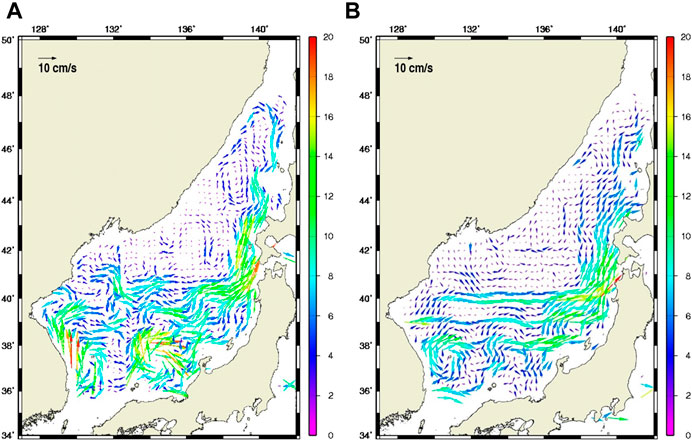
FIGURE 1. (A) Altimetry-derived surface current from AVISO and (B) geostrophic currents from EASRC in February.
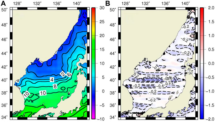
FIGURE 2. (A) Horizontal temperature distribution and (B) meridional temperature gradient at the surface of EASRC in February.
Therefore, this study reproduced and evaluated the same high-resolution field without this meridional gradient problem by using the optimal interpolation (OI) method. This problem has been observed in all seasons, but henceforth, this study will present the spatial distribution in February, when this problem is most evident.
The following section provides the data used, and details about the OI method implemented in this study. Results presents the meridional gradient patterns generated from several different OI versions. Summary and Discussion discusses the results and provides an overall summary.
Data and Methods
Data
This study used in situ World Ocean Database 2013 (hereafter WOD13) and gridded WOA13 data, which is the same as the recent version of the EASRC. All data are collected from NCEI as well. In the WOD13, we used the following datasets: Ocean Station Data (OSD), Mechanical Bathythermographs (MBT), Expendable Bathythermograph Data (XBT), High resolution Conductivity-Temperature-Depth (CTD), Drifting Buoy Data (DRB), Moored Buoy Data (MRB), Profiling Floats Data (PFL), Undulating Ocean Recorder Data (UOR), and Glider Data (GLD), https://www.ncei.noaa.gov/products/world-ocean-database) subject to the Quality Control (QC) procedure based on the NCEI technical report (Boyer and Levitus, 1994) and previous research (Chang et al., 2009).
First, the QC flag check of WOD13 data was performed and only good data were used in this study. Duplication and range checks for position, date, and pressure levels were carried out in the next step. Data that deviated from the standard range of temperature and salinity were eliminated and the density inversion check was also performed. WOD13 data includes observed level data and interpolated to a set of 102 standard levels. This study used standard level data observed from 1955 to 2012. We used a total of 1,443,820 profiles and 27,278 profiles have been rejected through the QC process. We also used the monthly mean of the WOA13 with a spatial resolution of 1° × 1° on 24 vertical levels from the surface to a depth of 1,500 m as background data to interpolate it even in areas where observations were scarce. It is to be noted that WOA was used similar to datasets on every 1° × 1° grid of the entire study area, eliminating the possibility of spatial imbalance in the final product. In this study, an objective analysis field for 19 vertical levels was generated using WOA13 with a 1° resolution and WOD13 observation data.
Method
In order to generate gridded temperature and salinity field at each depth, we employed the OI method as follows. The objective estimate (T(S)obj) of the temperature (salinity) at each grid point of standard depths is given by
where d = [d1, … ,dn]; it denotes the set of historical observed WOD13 and gridded WOA13 temperature (salinity) profiles on the grid point being interpolated and
Each historical WOD13 data
The covariance used in this study is a function of the spatial length scale (
Results
Reproduction of Meridional Gradient Problem
In order to investigate the possible cause of the meridional temperature gradient problem shown in the EASRC, similar meridional temperature gradient patterns must initially be reproduced.
The EASRC employed search passes within three circles of different radii (211, 155, and 111 km) to obtain a better representation of the objective analysis (OA) fields in this area, utilizing the response function of Barnes (1964). This study applied the same influence radius as the EASRC, but failed to represent any similar meridional temperature gradient problems, which may be related to differences in the OA method and datasets used after the QC procedure. Alternately, through multiple sensitivity experiments, an influence radius as 211 km in the longitudinal and 111 km in the latitudinal direction was set to reproduce the meridional temperature gradient problem. Several previous studies using the OI method applied a horizontal anisotropy scale, with Lx being greater than Ly, to reflect the predominant zonal currents in the ocean interior (Bohme and Send, 2005; Chang and Shin, 2012).
Figure 3 shows the OI result with a 0.1° grid resolution using both WOA13 and WOD13. The spatial distribution of temperature is very similar to that of the EASRC (Figure 2A), particularly with respect to the shape of the isothermal line and polar front position (Figure 3A). As for the meridional temperature gradient (dT/dy) shown in Figure 3B, strong negative values less than −0.2°C/km appeared at every 1° grid interval, from latitudes 38 to 41°N, with a minimum of about −0.6°C/km at 40°N. The average meridional temperature gradient by latitude was −0.32°C/km at 38°N, −0.37°C/km at 39°N, −0.77°C/km at 40°N, and −0.30°C/km at 41°N, which is similar to the mean temperature gradient of the EASRC (Figure 2B). This result indicates that the OI field generated by this study suitably reproduces the problem in the EASRC as shown in Figure 2B. We will further investigate the possible cause of the meridional temperature gradient problem, and provides the optimal OI fields without the same problem.
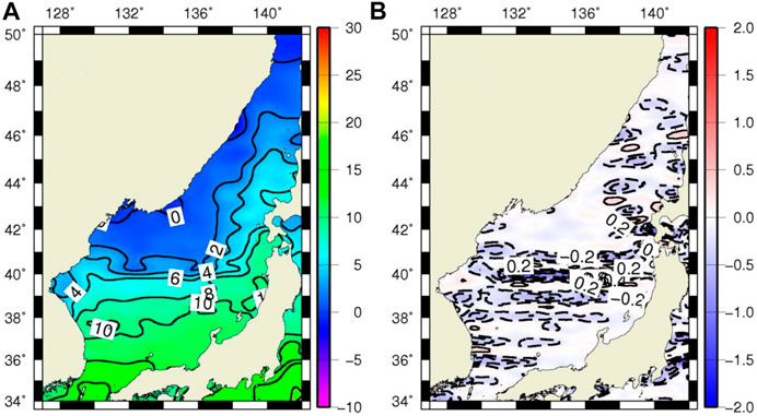
FIGURE 3. (A) Horizontal temperature distribution and (B) meridional temperature gradient at surface in February. This is a new optimal interpolation product with 0.1° resolution using both 1° gridded WOA13 and irregular WOD13. Influence radius applied was 211 km (zonal) and 111 km (meridional).
Effect of WOA13
We hypothesized that this abnormal meridional repetitive pattern was connected to the 1° by 1° grid WOA13 background data. Therefore, we generated a new OI field with the same influence radius using only WOA13 data (Figure 4). The spatial temperature distribution (Figure 4A) is smoother than in Figure 3A. Repetitive meridional gradient values less than −0.2°C/km can clearly be observed from latitudinal bands 38 to 41°N in Figure 4B. This anomalous pattern could be caused by the increased weight of WOA13 data at every 1° grid during the OI process for the generation of 0.1° high-resolution data.
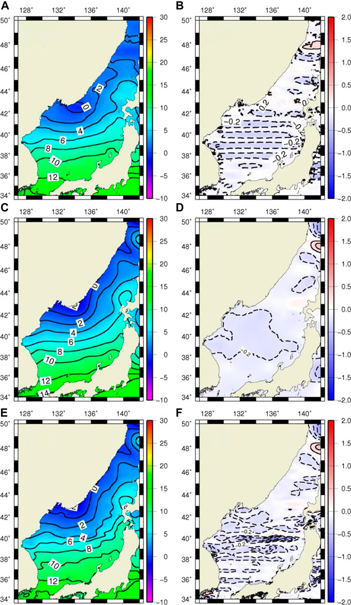
FIGURE 4. The same as Figure 3 except for (A, B) only 1° gridded WOA13, (C, D) only linear interpolated 0.1° WOA13, and (E, F) both 0.1° gridded WOA13 and irregular WOD13.
To rectify this, the WOA13 background data was reproduced on a regular 0.1° by 0.1° grid by using the linear interpolation method, and then OI was applied again (Figures 4C,D). Consequently, the temperature distribution was similar to the result using the 1° grid WOA13 data as previously shown in Figure 4A. However, the abnormal repetitive patterns of the meridional temperature gradient at 1° intervals clearly disappeared (Figure 4D). This implies that the abnormal meridional gradient problem can be corrected by using a relatively high-resolution climatology, such as WOA with a 0.25° resolution, GDEM, or WAGHC, rather than a 1° grid background field.
When the irregular in situ WOD13 data was supplemented for the OI process, it complicated the temperature distribution (Figure 4E). Interestingly, the abnormal meridional temperature gradient appeared again with a 1° grid meridional interval (Figure 4F).
Effect of WOD13
Based on the results depicted in Figure 4, we concluded that the repetitive temperature gradient pattern at 1° interval is affected not only by WOA13 data with a regular 1° grid but also by randomly distributed WOD13 data. In Figure 5, we regenerated OI fields just from WOD13 data and investigated its spatial distributions.
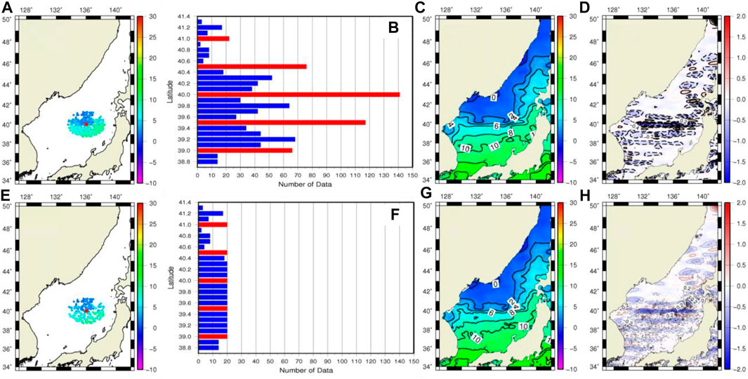
FIGURE 5. (A) Data position and (B) latitudinal change of the number of data within the influence radius of 136°E, 40°N, (C) horizontal temperature distribution, and (D) meridional temperature gradient by using only the irregular WOD13. Bottom panels provide the same information as the upper panels except for reduced WOD13 data that was randomly extracted for up to 20 profiles along 0.1° each latitudinal band within the influence radius.
Figures 5A,B show data distribution and the latitudinal change of the amount of data within the influence radius. A total 949 profiles were estimated within the influence radius of 136° E, 40° N. This position was selected because the largest meridional gradient value was noted at this latitude. Figures 5C,D show the spatial distribution of temperature and the meridional temperature gradient, respectively. The temperature distribution is similar to Figure 3A and the abnormal repetitive temperature gradient pattern at a 1° interval is also similar to that of Figure 3B. At the central latitude of 40° N, a total of 141 profiles were estimated within the zonal influence radius of 211 km. The number of data repeatedly increased at 1° intervals (see red bars in Figure 5B). Most ship observations were performed along the designated observation line, which ran predominantly along either latitudinal or longitudinal line. Consequently, the trend of number of observations along latitudinal lines being abundant remains consistent (see Figure 9). Thus, it is expected that the repetitive meridional temperature gradient pattern with 1° interval is closely related to the weighting of repetitive data numbers located at 1° grid intervals.
By randomly extracting WOD13 data of up to 20 profiles along 0.1° latitudinal intervals within the influence radius shown in Figures 5E,F, we produced another OI field. Figures 5G,H represent the temperature distribution and meridional gradient, respectively. Although data numbers constantly provided within the influence radius of every latitudinal band, results show that temperature distribution is similar to the previous version and that the repetitive gradient pattern still exists, but with decreased magnitude.
To confirm the weak relationship between spatial distributions of WOD13 data and the meridional gradient problem, this study generated another OI field using WOA13 data projected to a WOD13 position (Figure 6). Consequently, the temperature distribution is similar to the result obtained using WOA13 data with a regular 0.1° grid as previously shown in Figure 4C. In addition, the repetitive meridional gradient pattern at 1° grid intervals disappeared, which is consistent with the results shown in Figure 4D. We thereby confirmed that the cause of the meridional gradient problem is not closely related to the spatial distribution of WOD13 data.
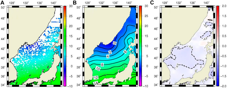
FIGURE 6. (A) Data position, (B) horizontal temperature distribution, and (C) meridional temperature gradient at the surface in February by using 0.1° WOA13 that was projected to a WOD13 position.
Effect of Influence Radius
Since this abnormal meridional gradient was reproduced accurately when we applied a horizontal anisotropy scale, we performed a sensitivity experiment with several influence radii having the same value in the zonal and meridional directions. Figures 7A,B depict the results of the new OI with an influence radius of 111 km in both zonal and meridional direction, based on the same two data (1° gridded WOA13 and irregular WOD13). Compared to Figure 3 which uses the same data except for a longer influence radius in the zonal direction, temperature distribution is more complicated especially along the 10°C isothermal line. However, the repetitive gradient pattern still exists, and is related to the same meridional influence radius of Figure 3.
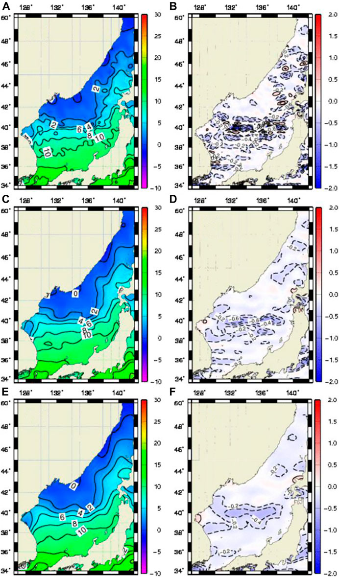
FIGURE 7. The same as Figure 3 except for three different influence radii. (A, B) The influence radius applied were 111 km, (C, D) 211 km, and (E, F) 311 km, respectively.
When we used the same 211 km influence radius in the zonal and meridional directions as shown in Figures 7C,D, the spatial distribution was similar to that of the existing OI results shown in Figure 3. In this case, repetitive patterns with a 1° interval in the meridional directions were significantly reduced. The same tendency was exhibited in the OI result using a 311 km radius circle (Figure 7F), but showed a smoother temperature distribution (Figure 7E).
One of the advantages of high-resolution climatology is its capacity to reproduce various meso-scale features. However, the smoothing effect due to the increased influence radius can lead to their disappearance. Therefore, we performed a wavelet analysis to determine the spatial variability of meso-scale features from the EASRC and various OI results, with the exception of the case using 111 km influence radius (Figure 7). Wavelet is a method of analyzing spectral characteristics over a period of time; however, in this study, we used it to analyze the characteristics of space by applying distance instead of time. The southwestern (northeastern) part of the East/Japan Sea was defined as the first (last) data position and the number of data position was increased in the meridional direction. In order to focus on the meso-scale features, we extracted the sea surface temperature anomaly (SSTA) by 230 km high-pass filtering.
Figure 8A shows the spectral density function of the SSTA in the EASRC. Figure 8B indicates the spatial-averaged spectral density function with a 95% confidence level. In the spatial-averaged spectral density function, a peak is appeared at a diameter of approximately 160 km which satisfies a 95% confidence level.
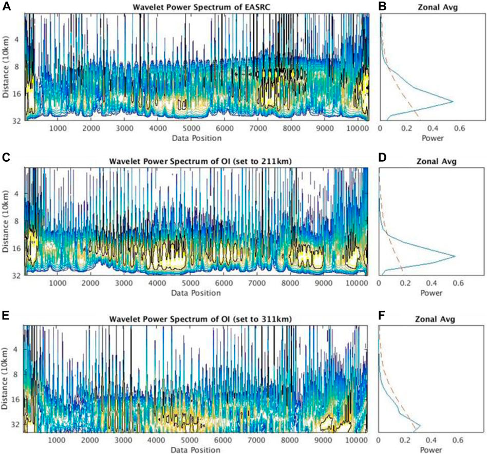
FIGURE 8. (A) Wavelet spectrum for sea surface temperature anomaly using Morlet wavelet with 95% significant confidence level (black line) in February of the EASRC and (B) spatial-averaged wavelet power spectrum with 95% significant confidence level (dotted line). The same information except for OI results are set to (C, D) 211 km and (E, F) 311 km.
For the new OI data, with an increased influence radius of 211 km in a meridional direction (Figure 7C), we performed the same analysis; the results are presented in Figures 8C,D. This, in contrast with the original EASRC in Figures 8A,B, shows similar results indicating the most significant peak on the meso-scale with a diameter of about 160 km within the 95% significant confidence level. Interestingly, the magnitude of the spatial-averaged spectral density function (0.58) is stronger than that of EASRC (0.55) in the 95% confidence level. In the original EASRC, various meso-scale features were not simulated due to the meridional temperature gradient problem. However, the new OI data with the influence radius of a circle of 211 km simulated various meso-scale features and solved the meridional temperature gradient problem.
As expected, another OI field using 311 km influence radius did not exhibit a peak in the spatial averaged spectral density function around 160 km within the 95% confidence level, and its amplitude was significantly reduced due to the smoothing effect (Figures 8E,F).
Therefore, OI results obtained by applying a circle of 211 km influence radius (hereafter “new OI”) in Figures 7C,D,8C,D showed that the abnormal temperature gradient problem has been resolved, and that the spatial variability in the meso-scale was well simulated. This result cannot prove that the new OI exhibits a real resolution of 0.1° that is a finer than meso-scale. We generated additional OI field using shorter period data for recent 20 years and investigated the spatial variability, but it also revealed the maximum spectral density around 160 km (not shown). It is inferred that the resolution of spatial variability will be more affected by the average period (less than monthly mean) rather than duration of data used. Therefore, it may be impossible to produce the monthly mean climatology simulating a fine scale about 0.1° in this area, which will be investigated in the further separate study.
Validation
We verified the EASRC and new OI field based on serial hydrographic lines that have been observed at the same position for a long time. One of the serial observation datasets was obtained from the 102, 103, 104, 105, 106, and 107 lines provided by the National Institute of Fisheries Science's Korea Oceanographic Data Center (NIFS/KODC) (the six lines of southwestern East/Japan Sea shown in Figure 9). The others represent the PM and G line data provided by the Japan Metrological Agency (JMA) (two lines of eastern East/Japan Sea shown in Figure 9). They have been simply averaged at each station from 1983 to 2010 for NIFS/KODC data and 1997 to 2010 for JMA data, respectively.
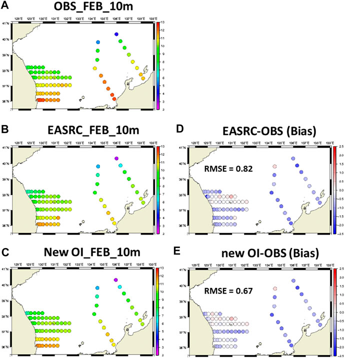
FIGURE 9. Spatial distribution of temperature and the bias with respect to serial observation at 10 m depth in February. [(A) Observation, (B) EASRC, (C) new OI, (D) EASRC-OBS, (E) new OI-OBS].
Figure 9 shows the spatial distribution of temperature in February, along the observational lines at 10 m depth obtained from long-term mean serial hydrographic data (Figure 9A), the EASRC (Figure 9B), and new OI fields with no meridional gradient problem generated by this study (Figure 9C). Since the surface data was relatively insufficient compared to the 10 m data shown in Figure 9A, verification was performed at 10 m instead of at the surface.
Both the EASRC (−0.61°C) and new OI (−0.44°C) show cold bias compared to the observation, which might be associated with an averaged period (Figures 9D,E). Both our climatologies contained many observations made before 1983 and 1997 based on WOD13 since 1955, therefore they reflect fewer of the recent sea warming signals in the East/Japan Sea. The root mean square error (RMSE) of the EASRC was 0.82°C, and the RMSE of the new OI was calculated to be 0.67°C. Thus, it was shown that the new OI was relatively similar to the observed data than the EASRC. This improvement is generally observed in different seasons (August) and depths (100 m depth) (see Supplementary Figures S1–S3). The objective of this study is to resolve the meridional temperature gradient problem as shown in the EASRC, rather than provide a synthetic assessment for the climatology, hence further detailed analysis is beyond the scope of this paper.
We also computed the geostrophic flow by using the new OI temperature and salinity profiles (Figure 10). The strong abnormal zonal flow that appeared in the original EASRC field has been significantly reduced. The East Korea Warm Current and the cold eddy near the Wonsan Bay were also resolved, and are now comparable to the AVISO data, as previously shown in Figure 1. The vector correlation coefficient between AVISO and the new OI was 0.54, showing a higher correlation than with the EASRC (0.52).
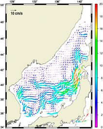
FIGURE 10. Spatial distribution of geostrophic currents from the new OI in February.
Summary and Discussion
This study found abnormal meridional temperature gradients from the East Asian Seas regional high-resolution climatology developed by NCEI and KODC and reproduced a similar high-resolution field by using the OI method. We used both WOD and WOA data to consider areas where observation data were insufficient.
In the results obtained using the OI method, the abnormal temperature gradient problem was partly related to the use of the WOA background field at the 1° grid. This problem was alleviated by employing a relatively high-resolution climatology background field less than 1° grid. In addition, it was significantly influenced by WOD data. When we examined the distribution of WOD data, we found that the number of data repeatedly increases along the 1° interval latitude band; however, this was not the main cause for the meridional temperature gradient problem. This problem was eliminated by increasing the influence radius in the meridional direction with respect to the existing influence radius. However, the EASRC data showing meridional temperature gradient problem also used similar circles with radii of 211, 155, and 111 km. Hence, it was inferred that changing the influence radius could not be a major solution for other OA products using different methods.
When we calculated the geostrophic current with the new OI field with the circle of 211 km influence radius, we found that strong zonal flows of 1° intervals are significantly reduced and they are similar to altimetry-derived surface current products. Moreover, spectral analysis using wavelet transform confirmed that despite the increased radius of influence in the zonal direction, the new OI maintains meso-scale variability suitably well compared to the original EASRC.
The latitudinal bands showing the strong repetitive meridional gradient pattern generally correspond to the movement of the polar front in the East/Japan Sea. Therefore, it is necessary to consider the interannual variability of the polar front when generating the monthly mean climatological fields. An improved climatological mean field can be produced when the effect of bottom topography reflecting potential vorticity change, and vertical gradient correction are considered (Chang and Shin, 2012; Chang and Shin, 2014). Moreover, this study including all NOAA climatologies produced the climatology mean field based on isobaric interpolation. Gouretski (2018), Gouretski, (2019) emphasized that the isobaric interpolation method produces “artificial water masses” in high-gradient regions. Since mixing processes in the actual oceanic environment occur along an isopycnal surfaces, if the isopycnal interpolation method is used instead of the isobaric interpolation method, an improved climatology mean field can be produced. More detail analyses are expected in this regard, via subsequent research.
In this study, this problem was solved by a different OA method from the EASRC. Therefore, we could not find a fundamental solution to the problem that emerges in the EASRC. Figure 11 shows spatial temperature distribution and the meridional gradient for the all the East Asian seas in the EASRC. Repetitive meridional gradient patterns are also found in the Yellow Sea and the East China Sea, but not in the southern part of Japan including the Northwestern Pacific. Therefore, to accurately complete the high-resolution climatology of the East Asian seas, it is necessary to analyze the features of each area (the East/Japan Sea, the Yellow Sea, the East China Sea, and the Northwestern Pacific) by applying different OA methods, including different radii of influence, and employing additional quantitative estimations.
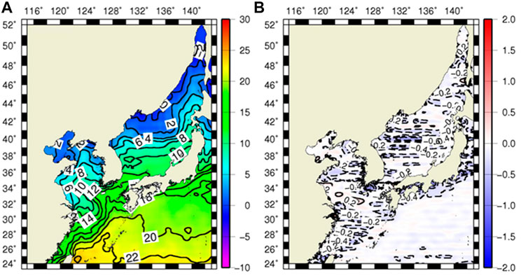
FIGURE 11. The same as Figure 2 except for the entire East Asian marginal seas.
Data Availability Statement
The original contributions presented in the study are included in the article/Supplementary Material, further inquiries can be directed to the corresponding author.
Author Contributions
Y-SC designed the study and J-HL carried out OI experiments. All authors contributed to the manuscript writing through discussion on the manuscript.
Funding
This research was supported by the National Research Foundation of Korea (2019R1A2C1008490) and Chungcheong Sea Grant Program founded by Korean Ministry of Oceans and Fisheries.
Conflict of Interest
The authors declare that the research was conducted in the absence of any commercial or financial relationships that could be construed as a potential conflict of interest.
Acknowledgments
We appreciate reviewers for insightful reviews of this paper.
Supplementary Material
The Supplementary Material for this article can be found online at: https://www.frontiersin.org/articles/10.3389/feart.2021.680881/full#supplementary-material
Supplementary Figure 1 | Spatial distribution of temperature and the bias with respect to serial observation at 100 m depth in February. [(A) Observation, (B) EASRC, (C) new OI, (D) EASRC-OBS, (E) new OI-OBS].
Supplementary Figure 2 | The same as Supplementary Figure S1 except serial observation is at 10 m depth for August.
Supplementary Figure 3 | The same as Supplementary Figure S1 except serial observation is at 100 m depth for August.
References
Barnes, S. L. (1964). A Technique for Maximizing Details in Numerical Weather Map Analysis. J. Appl. Meteorol. 3, 396–409. doi:10.1175/1520-0450(1964)003<0396:atfmdi>2.0.co;2
Böhme, L., and Send, U. (2005). Objective Analyses of Hydrographic Data for Referencing Profiling Float Salinities in Highly Variable Environments. Deep Sea Res. Part Topical Stud. Oceanography 52, 651–664. doi:10.1016/j.dsr2.2004.12.014
Boyer, T., Levitus, S., Garcia, H. E., Garcia, H., Locarnini, R. A., Stephens, C., et al. (2005). Objective Analyses of Annual, Seasonal, and Monthly Temperature and Salinity for the World Ocean on a 0.25° Grid. Int. J. Climatol. 25, 931–945. doi:10.1002/joc.1173
Boyer, T. P., Garcia, H. E., Locarnini, R. A., Zweng, M. M., Mishonov, A. V., Reagan, J. R., et al. (2018). World Ocean Atlas 2018. [indicate Subset Used]. NOAA National Centers for Environmental Information. Available at https://accession.nodc.noaa.gov/NCEI-WOA18.
Boyer, T. P., and Levitus, S. (1997). Objective Analyses of Temperature and Salinity for the World Ocean on a 0.25° Grid, 11. Washington, D.C: NOAA Atlas NESDISU.S. Gov. Print. Off.
Boyer, T. P., and Levitus, S. (1994). “Quality Control and Processing of Historical Temperature, Salinity and Oxygen Data,” in NOAA Technical Report No. 81 (Washington, D.C: U.S. Department of Commerce), 65.
Carnes, M. R. (2009). Description and Evaluation of GDEM-V3.0, NRL Memo. 7330-09-9165, 21. Mississippi: Naval Research Laboratory, Stennis Space Center, Miss. doi:10.2172/966897
Carnes, M. R., Helber, R. W., Barron, C. N., and Dastugue, J. M. (2010). Validation Test Report for GDEM4, Rep. NRL/MR/7330-10-9271. Arlington, Va: Space and Nav. Warfare Syst. Command. doi:10.21236/ADA530343
Chang, C.-W. J., and Chao, Y. (2000). A Comparison between the World Ocean Atlas and Hydrobase Climatology. Geophys. Res. Lett. 27, 1191–1194. doi:10.1029/1999GL002379
Chang, Y.-S., Rosati, A. J., Zhang, S., and Harrison, M. J. (2009). Objective Analysis of Monthly Temperature and Salinity for the World Ocean in the 21st century: Comparison with World Ocean Atlas and Application to Assimilation Validation. J. Geophys. RES. 114, C02014. doi:10.1029/2008JC004970
Chang, Y.-S., and Shin, H.-R. (2012). Objective Analysis of Monthly Temperature and Salinity Around the Southwestern East Sea (Japan Sea) on a 0.1° Grid. Continental Shelf Res. 45, 54–64. doi:10.1016/j.csr.2012.06.001
Chang, Y.-S., and Shin, H.-R. (2014). Vertical Gradient Correction for the Oceanographic Atlas of the East Asian Seas. J. Geophys. Res. Oceans 119, 5546–5554. doi:10.1002/2014JC009845
Fukumori, I., and Wunsch, C. (1991). Efficient Representation of the North Atlantic Hydrographic and Chemical Distributions. Prog. Oceanography 27, 111–195. doi:10.1016/0079-6611(91)90015-E
Gouretski, V. (2019). A New Global Ocean Hydrographic Climatology. Atmos. Oceanic Sci. Lett. 12, 226–229. doi:10.1080/16742834.2019.1588066
Gouretski, V. (2018). World Ocean Circulation Experiment - Argo Global Hydrographic Climatology. Ocean Sci. 14, 1127–1146. doi:10.5194/os-14-1127-2018
Johnson, D. R., and Boyer, T. P. (2015). Regional Climatology of the East Asian Seas: An Introduction, Vol. 79 Silver Spring, MD: NOAA Atlas NESDIS, 37.
Kim, K., Kim, K.-R., Min, D.-H., Volkov, Y., Yoon, J.-H., and Takematsu, M. (2001). Warming and Structural Changes in the East (Japan) Sea: A Clue to Future Changes in Global Oceans?. Geophys. Res. Lett. 28 (17), 3293–3296. doi:10.1029/2001GL013078
Levitus, S. (1982). “Climatological Atlas of the World Ocean,” in NOAA Professional Paper 13 (Washington, DC: U.S. Government Printing Office).
McIntosh, P. C. (1990). Oceanographic Data Interpolation: Objective Analysis and Splines. J. Geophys. Res. 95, 13529–13541. doi:10.1029/JC095iC08p13529
NOAA (1994). “World Ocean Atlas 1994, Vol. 1–5,” in NOAA Atlas NESDIS, Vol. 1–5 (Silver Spring, MD: NOAA).
NOAA (1998). “World Ocean Atlas 1998, Vol. 1 –12,” in NOAA Atlas NESDIS, Vol. 27– 38 (Silver Spring, MD: NOAA).
Pascual, A., Faugère, Y., Larnicol, G., and Le Traon, P.-Y. (2006). Improved Description of the Ocean Mesoscale Variability by Combining Four Satellite Altimeters. Geophys. Res. Lett. 33, L02611. doi:10.1029/2005GL024633
S. Levitus (2002). “World Ocean Atlas 2001, Vol. 1–6,” in NOAA Atlas NESDIS, Vol. 49-54 (Silver Spring, MD: NOAA).
S. Levitus (2006). “World Ocean Atlas 2005, Vol. 1–4,” in NOAA Atlas NESDIS, Vol. 61-64 (Silver Spring, MD: NOAA).
S. Levitus (2009). “World Ocean Atlas 2009, Vol. 1–4,” in NOAA Atlas NESDIS, Vol. 68-71 (Silver Spring, MD: NOAA).
Keywords: regional climatology, East/Japan Sea, horizontal temperature gradient, objective analysis, optimal interpolation, geostrophic current
Citation: Lee J-H and Chang Y-S (2021) Development of High-Resolution Regional Climatology in the East/Japan Sea With a Primary Focus on Meridional Temperature Gradient Correction. Front. Earth Sci. 9:680881. doi: 10.3389/feart.2021.680881
Received: 15 March 2021; Accepted: 16 June 2021;
Published: 02 July 2021.
Edited by:
Andrea Storto, Institute of Marine Science (CNR), ItalyReviewed by:
Viktor Gouretski, Chinese Academy of Sciences, ChinaGilles Reverdin, Center National de la Recherche Scientifique, France
Copyright © 2021 Lee and Chang. This is an open-access article distributed under the terms of the Creative Commons Attribution License (CC BY). The use, distribution or reproduction in other forums is permitted, provided the original author(s) and the copyright owner(s) are credited and that the original publication in this journal is cited, in accordance with accepted academic practice. No use, distribution or reproduction is permitted which does not comply with these terms.
*Correspondence: You-Soon Chang, eXNjaGFuZ0Brb25nanUuYWMua3I=