 Amit Kumar
 Naresh Kumar
 Sagarika Mukhopadhyay1*
 Simon L. Klemperer
- 1Department of Earth-Sciences, IIT Roorkee, Roorkee, India
- 2Geoscience, National Centre for Polar and Ocean Research, ESSO, Ministry of Earth Sciences, Government of India, Headland Sada, Vasco Da Gama, India
- 3Wadia Institute of Himalayan Geology, Dehradun, India
- 4Department of Geophysics, Stanford University, Stanford, CA, United States
The major scientific purpose of this work is to evaluate the geodynamic processes involved in the development of tectonic features of NE India and its surroundings. In this work, we have obtained tomographic images of the crust and uppermost mantle using inversion of Rayleigh waveform data to augment information about the subsurface gleaned by previous works. The images obtained reveal a very complicated tectonic regime. The Bengal Basin comprises a thick layer of sediments with the thickness increasing from west to east and a sudden steepening of the basement on the eastern side of the Eocene Hinge zone. The nature of the crust below the Bengal Basin varies from oceanic in the south to continental in the north. Indo-Gangetic and Brahmaputra River Valleys comprise ∼5–6-km-thick sediments. Crustal thickness in the higher Himalayas and southern Tibet is ∼70 km but varies between ∼30 and ∼40 km in the remaining part. Several patches of low-velocity medium present in the mid-to-lower crust of southern Tibet along and across the major rifts indicate the presence of either partially molten materials or aqueous fluid. Moho depth decreases drastically from west to east across the Yadong-Gulu rift indicating the complex effect of underthrusting of the Indian plate below the Eurasian plate. Crust and upper mantle below the Shillong Massif and Mikir Hills are at a shallow level. This observation indicates that tectonic forces contribute to the uprising of the Massif.
Key Points
1. Our new Rayleigh wave tomography of NE India provides a 3D view of the complex interaction between Indian, Asian, and Burma plates.
2. Moho geometry shows expected crustal thinning beneath Bengal Basin and thickening beneath the Himalayas, but also pronounced Moho shallowing beneath Shillong Plateau/Mikir Hills.
3. Low-velocity bodies in the mid-crust of southern Tibet/Lhasa blocks likely indicate partial melts or fluids that are not only restricted to beneath the narrow surface graben.
Introduction
A long span of convergence between Indian and Eurasian plates has caused subduction, under-thrusting, and extrusion resulting in widespread lithospheric deformation (Molnar et al., 1977; Molnar, 1984; Tapponnier et al., 2001; DeCelles et al., 2002; Nábeˇlek et al., 2009). Recently and in the past, the NE Indian region has experienced a frequent occurrence of moderate to large-size earthquakes due to ongoing active tectonic convergence (Ni and Barazangi, 1984; Pandey et al., 1995; Parvez and Ram, 1997; Kayal, 2008; Baruah et al., 2014, 2016; Le Roux-Mallouf et al., 2020). In response to the collision, the lithospheric part of these three plates experiences horizontal shortening and surface uplift. Elevated Tibetan plateau, Indo-Burma Ranges (IBR), and the Himalayas are the result of the collision and crustal thickening, which is associated with mountain building phenomena and crustal shortening (Burchfiel and Royden, 1985; England and Houseman 1989; Murphy and Copeland, 2005; Thiede et al., 2006). The study region includes Brahmaputra River Valley (BRV), Shillong Massif (SM), Mikir Hills (MH), Indo-Burma Ranges (IBR), Bengal Basin (BB), southern Tibet, eastern Himalayas, and part of central Himalayas (Figure 1A), characterized by the diverse geological setup and a very high variation in topography. The overall study region is demarcated by latitude 22°N to 32°N and longitude 85°E to 98°E. Detailed geological and tectonic studies were carried out by Krishnan (1960), Evans (1964), Desikachar (1974), and Nandy (1980).
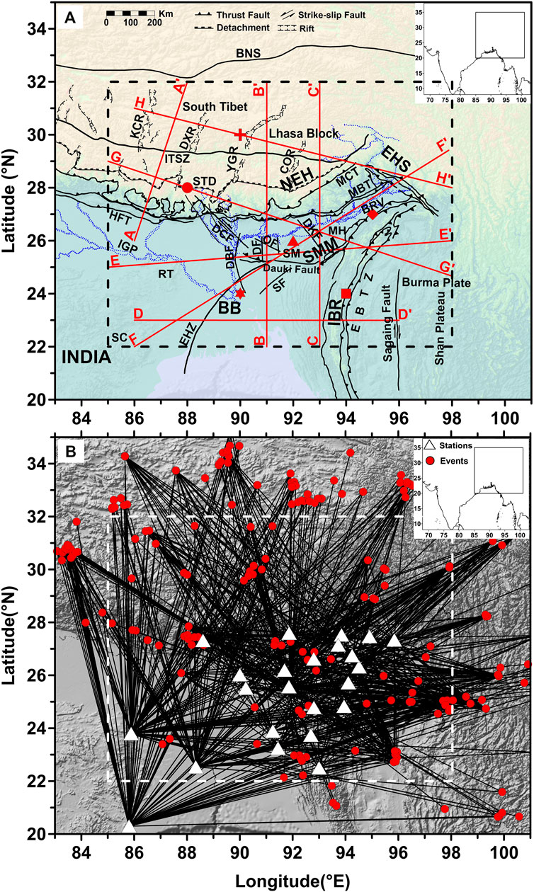
FIGURE 1. Tectonic map of NE India and the surrounding area (GSI, 2000). Red symbols (shapes same as corresponding curves): location of six points for which Rayleigh wave dispersion curves are shown in Figure 4. Red lines: location of profiles for S-wave structures (Figure 8). Rectangle (dash line) encloses the area for which results are used for interpretation. Abbreviations—IBR: Indo-Burma Ranges; NEH: Northeastern Himalaya; EHS: Eastern Himalayan Syntaxis; SMM: Shillong-Mikir Massif; SM: Shillong Massif; MH: Mikir Hills; BRV: Brahmaputra River Valley; BB: Bengal Basin; EBTZ: Eastern Boundary Thrust Zone; BNS: Bangong-Nujiang Suture; ITSZ: Indus-Tsangpo Suture Zone; STD: Southern Tibetan Detachment; MCT: Main Central Thrust; MBT: Main Boundary Thrust; HFT: Himalayan Frontal Thrust; IGP: Indo-Gangetic Plain; SC: Singhbhum Craton; RT: Rajmahal Trap; SF: Sylhet fault; DBF: Dhubri fault; DKF: Dhansiri-Kopili fault; DF: Dudhnoi fault; EHZ: Eocence Hinge Zone; OF: Oldham fault; KCR: Kung-Co Rift; DXR: Dinggya-Xainza Rift; YGR: Yadong-Gulu Rift; COR: Cona-Oiga Rift; DCF: Dhubri-Chungthang Fault Zone. (B): Location of epicenters (solid red circle) and stations (white triangle) used for this study. Event-station path coverage at 12 s period is shown by black lines. Inset: Map of India showing the study region. Only those earthquakes are shown whose data are used in this analysis.
In NE India, the Indian plate is supposedly simultaneously underthrusting beneath Eurasia and subducting below Burmese microplate in the north and east, respectively (Kayal, 2008; Sarkar et al., 2013; Kumar et al., 2015; Raoof et al., 2017). Le Dain et al. (1984) proposed that in the early Cenozoic period, the Indian plate subducted below the Burma microplate and presently the hanging lithosphere is being dragged northward. Mukhopadhyay and Dasgupta (1988), Kayal (1989, 1996), and Satyabala (2003) opined that the Indian plate is actively subducting below the Burma plate. GPS measurements in this area and Myanmar suggest EW convergence with a shallow dip of the Indian plate beneath Myanmar, which is locked along a megathrust further down-dip (Gahalaut et al., 2013; Steckler et al., 2016). Steckler et al. (2016) and Gahalaut et al. (2013) suggest that the active subduction has stopped, whereas Steckler et al. (2016) inferred active subduction despite the highly oblique plate motion and presence of thick sediment.
The convergence of Indian and Eurasian plates causes N-S compression mainly within the Himalayas and E-W extension within the Tibetan plateau (Armijo et al., 1986; Angelier and Baruah, 2009; Sarkar et al., 2013). Several workers suggested that low-velocity material is present within southern Tibet as a result of EW extension along several rifts (Kind et al., 1996; Cogan et al., 1998; Jiang et al., 2014) due to clockwise deformation with respect to the northeast corner of NE India. Extension-related normal faults have been identified (Kayal, 2001, 2008; Hintersberger et al., 2010) mostly within the Tibetan plateau and also in some cases in the Higher and Lesser Himalayas. Focal mechanism solutions in the eastern Himalayas expose the direction of compression from NNW-SSE to N-S from Arunachal Pradesh, Mishmi hills to Bhutan. However, in the IBR, NE-SW directed average compression is observed (Angelier and Baruah, 2009). IBR is under compression due to oblique subduction of the Indian plate below the Burma plate, where the NE-SW directed stress across the inner and northern arc is switched to the E-W directed stress near the Bengal Basin. Within NE India and SM, Baruah et al. (2016) made an investigation on tectonic stress through inversion of the stress tensor. They observed that compressional stress direction changes from NNW-SSE in the western part of the massif to the NNE-SSW direction in its eastern part. Oblique subduction of the Indian plate underneath the IBR causes compression along the NNE-SSW direction (Baruah et al., 2013, 2016). The available data set make it possible to study the crustal and upper mantle structure of Lhasa/southern Tibet and IBR.
Eastern Himalayan syntaxis (EHS) is a complex triple junction of Indian and Eurasian plates with the northern end of the Burma plate (Curray, 1989). A study of active tectonics in EHS was done by Holt et al. (1991). They identified an oblique thrust based on focal mechanisms and it shows the movement of the Indian plate directed toward NNE as it underthrusts below this region. Baranowski et al. (1984) found that radial directed slip in the Himalayas causes extension within Tibet; however, it is possibly half of the rate of under-thrusting taking place within the Himalayas. Holt et al. (1991) found that slip vectors are generally not orthogonal to the strike of the Himalayas.
Different workers have proposed different tectonic processes for the formation of SM. Evans (1964) postulated that the Dauki fault is a strike-slip fault along which SM has moved ∼250 km eastward to its present position. Oldham (1899) concluded that movement along a thrust-plane or thrust planes and along secondary thrusts and fault planes may be the cause of the 1897 great Earthquake. Bouguer and isostatic anomalies indicate that high-density crustal/upper mantle strata are present beneath SM (Verma and Mukhopadhyay, 1977). Kailasam (1979) suggested that isostatic adjustment may have caused uplift of SM but positive Bouguer and isostatic anomalies over it imply that it should sink. Dziewonski and Anderson (1983) estimated the P-wave travel time residual beneath the Massif to be −0.57 s, indicating that the subsurface has higher velocity material than the surroundings. Many researchers suggested that the uplift of SM is influenced by active tectonics between NE India and the NE Himalayas (Chen and Molnar, 1990; Khattri et al., 1992; Mukhopadhyay et al., 1993, 1997; Najman et al., 2016; Govin et al., 2018). Mukhopadhyay et al. (1997) opined that the Massif has overthrusted southward above the Indian plate along the Dauki fault. Bilham and England (2001) and England and Bilham (2015) proposed that SM uplifted abruptly by ∼11 m during the 1897 Shillong earthquake and suggested that it is a “pop-up” structure, whereas Raoof et al. (2017) suggested that it is the crest of the buckled-up part of the Indian plate. Clark and Bilham (2008) suggested that convergence of India and Eurasia in this part is shared between the Bhutan Himalayas and the Shillong Massif. Strong et al. (2019) stated that the Massif is affected by active uplifting as well as erosion.
From this discussion, it is obvious that there are several postulates about the tectonics and geodynamic characteristics of this area that has led to such a complex crustal/lithospheric structure. Hence, this area needs detailed investigation. The availability of a dense seismic network in NE India makes it possible to carry out such investigations for this region. The study region is selected because it shows complex variations in plate motion that may affect the subsurface structure and properties of the lithosphere. In this study, we decipher subsurface characteristics to understand the effects of NS underthrusting and EW subduction in NE India and its surroundings. Most of the geophysical investigations were carried out on collision zones either toward the north or northeast of SM (Singh et al., 2015 and the references therein). However, the southern side of SM and that of BB have not been studied much due to unavailability of sufficient data. Thick sediments within BB make it challenging to delineate the underlying oceanic and/or continental crust (Alam et al., 2013). Sediment thickness and crustal structure of BB have been investigated by Currey (1991), Brune et al. (1992), Mitra et al. (2011), and Singh et al. (2016). The extent of sediment deposition and the nature of the crust in BB are required to be properly investigated. We have estimated the lateral variation in sedimentary layer thickness in BB. Although Bangladesh seismological data were not incorporated in the present work, there are stations in the surrounding part of India that gave good coverage of this zone.
We made use of new data sets covering NE India and surrounding areas and tried to solve several issues, such as Moho depth variation, nature of crust and sedimentary layer thickness variation in BB, deformation, and upliftment of SM in response to active NS and EW compression, geodynamic inferences related to oblique subduction of Indian plate below IBR, indentation of EHS and occurrence of low-velocity material in mid-crust of SE Tibetan plateau. To obtain the subsurface crustal and lithosphere S-wave velocity (Vs) image of the study area, surface wave tomography technique developed by Ditmar and Yanovskaya (1987), Yanovskaya and Ditmar (1990), and Yanovskaya et al. (1998) is applied. Tomographic image of the study area is obtained up to ∼90 km depth, which elucidate the geodynamics of NE India through high-resolution data.
Data
Surface wave data recorded by a network of 20 broadband seismic stations in NE India and three other stations (Kolkata, Bhubaneswar, and Bokaro) operated by the India Meteorological Department (IMD, India) were used in the present study (Figure 1B; Table 1). The last three stations provide better path coverage for BB. The instruments used in these seismic stations (Table 1) include Trillium-240, STS-2, RT151-120, and CMG40T with natural periods of 240, 120, 120, and 30 s, respectively. The data for 201 earthquakes (Figure 1B, Supplementary Table S1) used for this study were recorded at local and regional epicentral distances in the range of ∼160–∼1800 km. Surface waves of good signal strength recorded for wave period >1 s generated by earthquakes of focal depth ≤50 km and magnitude ≥5 were used. Shallow focal depth earthquakes generate higher surface wave amplitudes, and therefore even lower magnitude (M∼5) records at regional distances have good surface wave signals. Based on selected stations and event locations, we have obtained maximum 753 source–receiver paths (Figure 1B; Table 2), which covers a broad range of azimuths and path lengths within the area of investigation. Supplementary Figure S1 shows ray path coverage for periods between 8 and 60 s.

TABLE 1. Detail information of seismic stations.
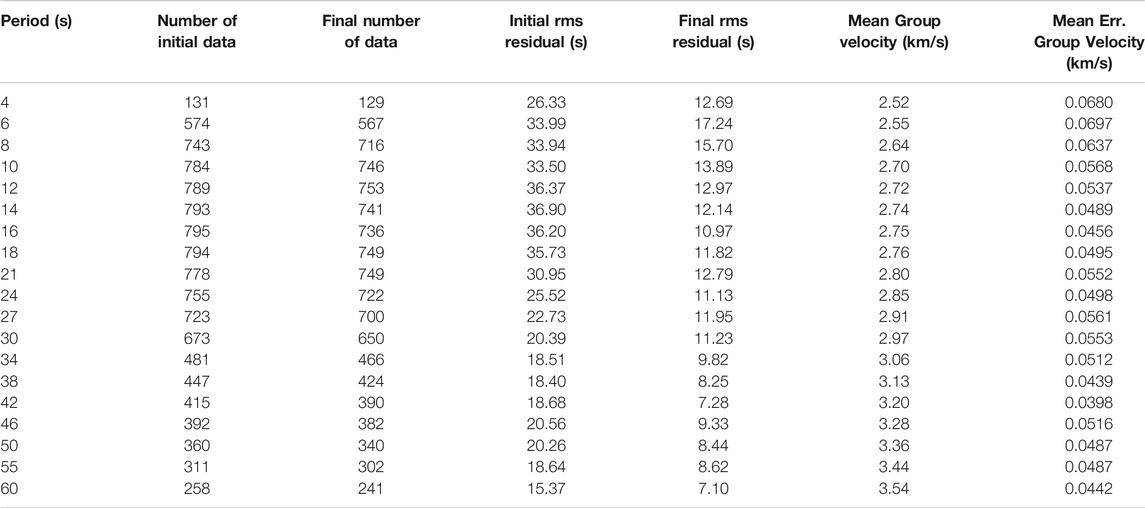
TABLE 2. Group-velocity tomographic inversion details. Number of data (paths), final number of data after excluding outliers, initial rms residual (before tomography), final rms residual (after tomography), and averaged group velocity after tomographic inversion for different periods with mean error.
Data processing was performed in four steps: 1) estimation of fundamental mode Rayleigh wave dispersion curves, 2) construction of group velocity maps at different grid points of specified spacing for good resolution, 3) inversion of dispersion curve of each grid for obtaining 1D S-wave (Vs) velocity structure, and 4) construction of 2D and 3D images of Vs.
Estimation of Group Velocity
Pre-processing steps were carried out to remove the mean value, linear trend, and avoid spectral leakage (using tapering window) from raw data. The data were also converted into ground motion (displacement) units using the frequency response of the recorders. Fundamental mode dispersion curves of Rayleigh wave were estimated along each path between earthquake epicenter and the seismic station using the multiple filter technique (MFT) developed by Herrmann (2013) and Herrmann and Ammon (2002) based on the methodology of Dziewonski et al. (1969). MFT is a fast and efficient method used for analyzing multiple dispersed signals (Herrmann, 1973; Erduran et al., 2007). In this method, the Fourier transform of the signal selected for a given time window displays amplitude variation with frequency. In the next step, Gaussian filter is applied and followed by inverse Fourier transform to obtain the peak of the spectrum for a given time and frequency. The MFT uses phase-matched filtering to extract the dispersed waveform. It separates the other parts of waveform consisting of body waves, higher modes, and multipath effects (Kolinsky, 2004). Examples of dispersion curves are given in Figure 2.
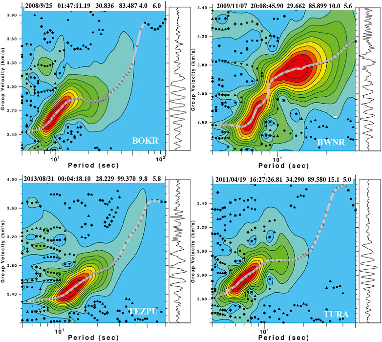
FIGURE 2. Examples of dispersion curves obtained at four stations. Earthquake source parameters and the recording station names are mentioned on the dispersion curve plot. The range of the data of the dispersion curve used for further analysis is shown with a gray-color curve. The color in a particular contour defines the energy with blue representing minimum energy and its energy increasing trend from blue to cyan to green to yellow to red. Raw waveform is given in the right-hand rectangular block.
Selection of range of periods of dispersion curves is based on the natural period of the seismometer, data sampling rate, noise level, and the distance between the epicenter and station along the great circle arc (Yao et al., 2006; Bensen et al., 2007; Yang et al., 2007; Guo et al., 2009; Kumar et al., 2017). The upper limit of the period up to which group velocity can be estimated also depends on the ratio of epicentral distance and the maximum wavelength of the recorded signal. The reliable maximum period of surface wave recorded at a given epicentral distance should have at least three wavelengths within that distance (Yao et al., 2006; Bensen et al., 2007; Yang et al., 2007; Guo et al., 2009). Based on these criteria, we could extract dispersion data for periods between 4 s and 60 s. Wave propagation path coverage for a particular period depends on the availability of good quality data. Path coverage in this study region varies (Supplementary Figure S1), and it has a maximum value at 12 s period (Figure 1B). In total, maximum 795 Rayleigh wave records were used. Minimum and maximum numbers of paths used for tomographic inversion of group velocity values are 129 and 753 at periods of 4 s and 12 s, respectively (Table 2).
Group Velocity Tomography
Tomographic Inversion Method
Surface wave dispersion data were used to generate a map of spatial variation of group velocity for different periods within the study region. Surface wave velocity tomography maps are constructed through the inversion technique developed by Ditmar and Yanovskaya (1987) and Yanovskaya and Ditmar (1990). Dispersion curves obtained from the earthquake data are path specific, that is, each one gives average group velocity versus period for that particular path between earthquake epicenter and station location. It gives the group velocity for a particular period at different grid points of the study region. This inversion technique is robust and does not need any initial parameterization or truncation of Taylor series expansion of nonlinear equation because of its straightforwardness (Levshin et al., 1989). The basis functions for the inversion model are formed as a superposition of kernels of the group velocity travel time integral (Ritzwoller and Levshin, 1998). Measured group velocity is a function of the location described by U(θ,ϕ) on a spherical surface. It is decomposed in different sections across the study region by taking the mean group velocity as a starting value and applying region-specific perturbations. Decomposed reference value U0 and its location dependence perturbation are expressed by
Initially, this method leads to a search for smooth perturbation in group velocity from the reference model U0 so that U(θ,ϕ) gets fitted by N observed group travel times
Here, Pi is the ith wave path, wi is the associated weight through a map of group velocity U(θ,ϕ),
Tomographic images of Rayleigh wave group velocity were obtained at periods ranging between 4 s and 60 s on 1° × 1° grid spacing. The regularization parameter is chosen such that the velocity range in the group velocity maps is identical or larger than the range of measured group velocities (Yanovskaya et al., 1998). To obtain an appropriate smoothed map, we have used several regularization parameters (
For best results in a tomographic study, the area of investigation should be covered uniformly by ray paths from all directions. Unfortunately, that is very rarely possible. Uneven distribution of ray paths may introduce some anomalous values to the solution. The solution is obtained after rejecting the data of a path with anomalous values categorized based on regularization parameters. The anomalous value represents a large deviation from the average velocity of a particular localized region. This error may be due to unresolvable lateral velocity variations, measurement errors, multipath effects, etc. (Yanovskaya and Kozhevnikov, 2003). The quality of the solution for the given regularization parameter is measured by comparing the initial and the remaining (unaccounted) mean square travel time residuals (Yanovskaya et al., 1998). Here, the initial means the travel time residual before the inversion based on the mean velocity of the data. The value of standard error (σ) was used for data selection. If an individual value of the travel time residual shows the value laying more than 3σ, the corresponding data were rejected from the data set and further recalculation of the solution is done. The observed values are almost comparable to the a priori errors resulting in fine velocity maps (Table 2). The standard errors associated with the evaluated group velocities are ≤0.07 km/s.
Ditmar and Yanovskaya (1987) and Yanovskaya et al. (1998) used two parameters, viz., mean size and stretching (ε) of the averaging area to prioritize lateral resolution. Yanovskaya (1997) adopted a technique similar to the one formulated by Backus and Gilbert (1968) for the 1D problem. This is formulated for 2D inversion through the calculation of the size of the averaging area S(x,y) for each point in different directions. Obtained resolution approximated by an averaging area over an ellipse centered at the point with Smax (x,y) and Smin(x,y) as the largest and smallest axes, respectively, over the area S (x,y) (Karagianni et al., 2002; Yanovskaya and Kozhevnikov, 2003). The mean size of the averaging area, L=(Smax + Smin)/2, is the measure of the resolution for a particular point and these values for all grid points was used to calculate the lateral resolution of the area under investigation. The resolution depends on the path coverage between the epicenter and station as well as its azimuthal distribution (Gonzalez et al., 2007). The lateral resolution of the mean of the average area is less than 200 km in most of the regions under investigation (Figure 3A and Supplementary Figure S4A). The lateral resolution for the present data set was evaluated for different periods between 4 and 60 s. Its variation for a set of four periods (8, 12, 30, and 60 s) is shown in Figure 3A. Plots for the remaining periods are shown in Supplementary Figure S4A. It is noticed that the resolution is good between the 8 s and 30 s period. The evaluated 2D resolution dimension mainly portrays the propagation path geometry and its density as shown in Figure 1B; Supplementary Figure S1.
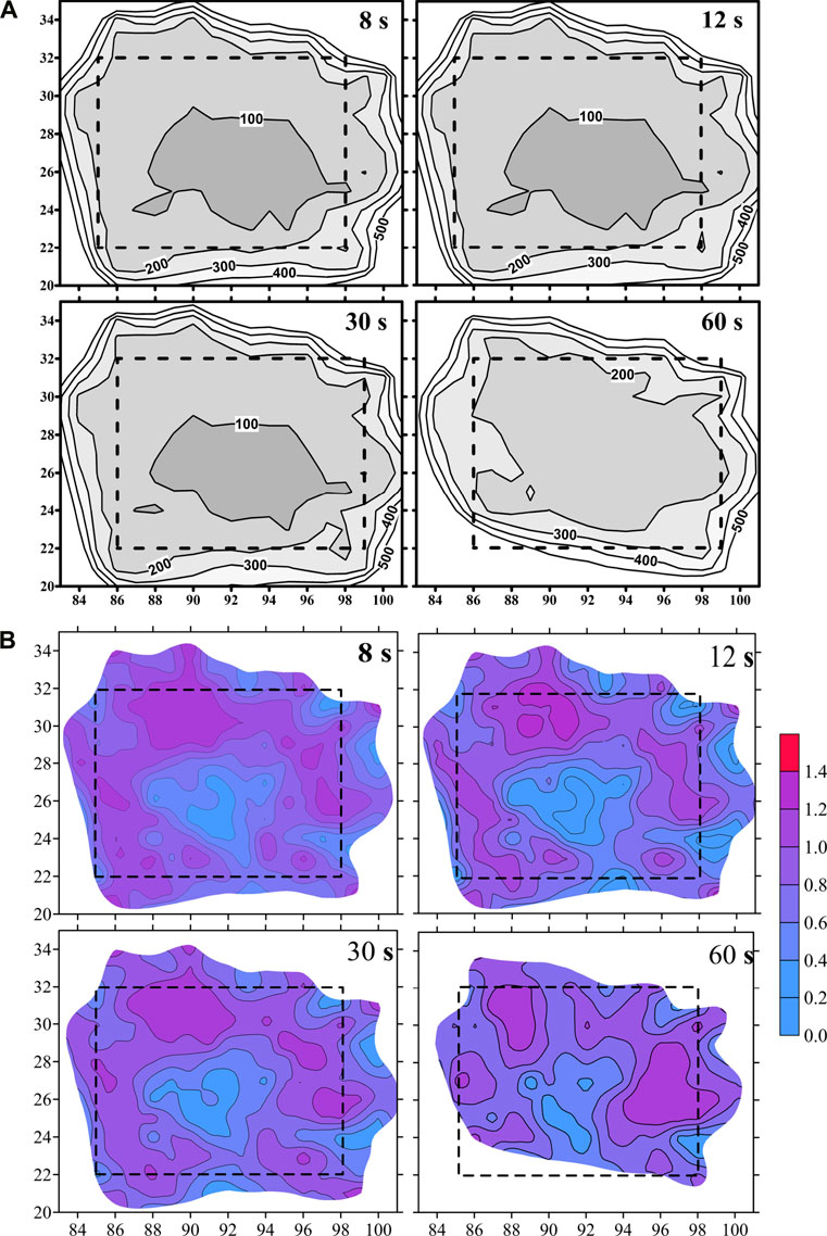
FIGURE 3. Contoured diagrams of (A) mean size of averaging resolution length (in km) and (B) distribution of stretching parameter. Areas, where the resolution length of tomographic image >200 km, are clipped and shaded white. An area having a good resolution is demarcated by a rectangular box marked with dashed lines.
The stretching parameter (ε) indicates how uniform the spatial distribution of the path is (Gonzalez et al., 2007). The stretching (ε) of the averaging area is obtained by 2(Smax (x,y)-Smin(x,y))/(Smax (x,y)+Smin(x,y)), which describes the quality of the source–receiver path coverage (Kumar et al., 2019). Small values of the stretching imply that the paths are uniformly distributed in all directions, whereas large values indicate a preferred orientation of paths (Yanovskaya, 1997). Areas with stretching values ≤ 1.0 are considered to have a uniform azimuthal distribution of path and resolution is nearly the same along all directions. Figure 3B and Supplementary Figure S4B show stretching for the same periods for which resolution has been plotted. Tomographic images for group velocity and Vs are shown later for only the part where the resolution, as indicated in Figure 3A; Supplementary Figure S4A, is good.
Tomographic Images
Rayleigh wave group velocity tomograms for 16 different periods were obtained at 4, 6, 8, 10, 12, 16, 21, 27, 30, 34, 38, 42, 46, 50, 55, and 60 s to measure the spatial variation. Tomographic images are shown for the area where the spatial resolution is good (i.e., the mean size of the averaging area L ≤ 200 km). This encloses the area covered by the dense ray paths (Figures 1B, 3A, and Supplementary Figure S1). Local dispersion curves obtained through tomography for six grid point locations (Figure 1A) are shown in Figure 4 that indicates a high variation of group velocities at different periods from one place to another. Eight group velocity tomograms at 6, 10, 16, 24, 30, 38, 50, and 60 s are shown in Figure 5, and the rest are plotted in Supplementary Figure S5.
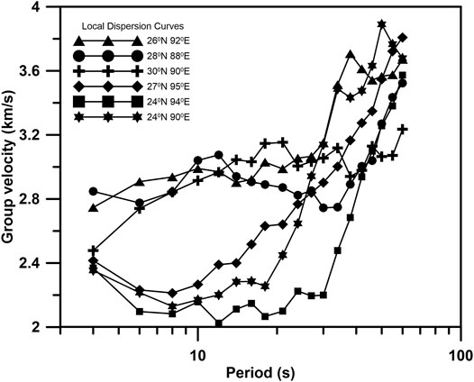
FIGURE 4. Local dispersion curves for six different grid points (locations shown in Figure 1A).
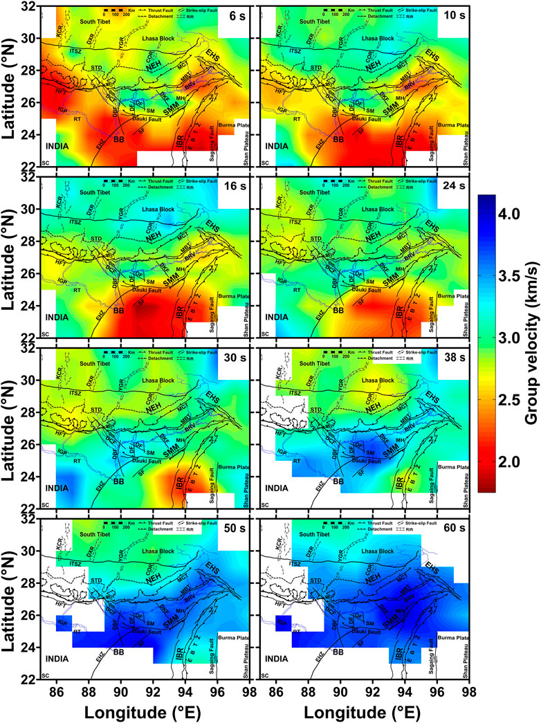
FIGURE 5. Rayleigh wave fundamental mode group velocity tomographic images at different periods. Areas, where the resolution length of tomographic image >200 km, are clipped and shaded white.
Rayleigh wave group velocity varies between ∼1.80 km/s and ∼4.15 km/s for periods ranging between 4 s and 60 s (Figure 5; Supplementary Figure S5). The data set is enough to investigate the crustal and uppermost mantle structures of the study region. Lateral variations of group velocities represent different geological and tectonic features. A shorter period of the Rayleigh wave group velocity map is very sensitive to Vs in the uppermost crust, whereas a longer period has deeper depth sensitivity depending on its wavelength. Lateral variation of group velocity can be discussed based on various geotectonic features.
According to Mitra et al. (2006), group velocities at <22 s periods represent upper crust, between 25 s and 35 s are mainly influenced by lower crust and up to 60 s represents upper mantle structure. Figure 4 shows that dispersion curves obtained for grid nodes (Figure 1A) located in the BB, IBR, and BRV have lower group velocity values at lower periods compared to those located at SM, STD, and Lhasa block. This indicates the effect of sediments at shallower depths in BB, IBR, and BRV regions. The rate of increase of group velocity value at periods greater than 20 s is very high except for the Lhasa block, indicating the presence of a low-velocity medium in lower crustal depth in the Lhasa block.
At periods ≤10 s, the entire BB, Indo-Gangetic Plain (IGP), eastern Nepal Himalayas, IBR, and parts of southern Tibet show low group velocity values (Figure 5, Supplementary Figure S5). At 12–16 s, the values are still low for BB and the southern part of IBR. The low-velocity up to ∼24 s Dhubri-Chungthang Fault Zone (DCF) demarcates a boundary suggesting a change in the sub-surface structure in the crust with similar observations by Diehl et al. (2017). The low-velocity zone systematically shifts south-eastward toward the southern part of the IBR with an increase in the period from 16 s to 42 s, and the group velocity value also increases within this zone with increasing period. The very low group velocity values (red color, Figure 5, Supplementary Figure S5) indicate the presence of sedimentary rocks. As group velocity at a higher period is affected by the Vs of the medium at greater depth, this shows that sedimentary rocks are present in BB and the southern part of the IBR up to greater depth. This observation for BB is supported by earlier investigations (Verma and Mukhopadhyay, 1977; Mitra et al., 2006; Acton et al., 2010), but for IBR, this is new information. Shifting of low group velocity from BB to IBR is supportive evidence of oblique subduction (Mitchell and McKerrow, 1975; Curray, 1989; Ni et al., 1989) of the Indian plate below the Burma plate. A higher velocity gradient in the western part of the BB relative to the eastern part of it shows that the basement depth increases from west to east. Low group velocity (from 4 s to 16 s) in BRV and IGP is also evidence of the presence of sediment at shallow depth (Kumar et al., 2018a). Kayal (2008) reported that the average sediment thickness in BRV is ∼4 km. No anomalous change is found in this zone and a continuous increase in group velocity is observed, indicating a gradual increase in medium velocity with depth. The Singhbhum craton and Rajmahal trap in the Indian shields in the southwestern part of the study region are represented by relatively higher group velocity up to 30 s. A prominent increase in group velocity from 21 s along the NE direction of the Indian continent to SMM and EHS is observed. It may reflect upward crustal buckling at the middle of the study region as suggested by Raoof et al. (2017).
At all periods, SMM shows up as a zone of high group velocity indicating the presence of high-velocity crystalline rock bodies at all depth levels. A sudden decrease in group velocity is observed across the Dauki fault from north to south up to 21 s period. At periods >30 s, southern Tibet has lower group velocity compared to eastern Himalayas, NE India, and BB, indicating that at a deeper depth, the former region comprises lower velocity material. This corroborates the presence of thick crust in Tibet. This is also in accordance with the suggestion of the presence of partial melts and/or aqueous fluids in the mid-crust in Tibet (Brown et al., 1996; Cogan et al., 1998; Hetényi et al., 2011; Jiang et al., 2014). Such low-velocity zones in southern Tibet are observed in between 27 s and 50 s. Acton et al. (2010) also observed this type of change of velocity pattern between 50 s and 70 s and inferred that the crust below the Tibetan plateau is thick. Variation of group velocity all along the Himalayas, especially at lower periods, indicates the possible variation of crustal thickness along this tectonic trend as suggested by Raoof et al. (2017). In Nepal Himalayas, the low-velocity at short period has also been observed by Guo et al. (2009). The Gangetic plains adjacent to this region also have relatively lower group velocity with high gradients up to 16 s, which is similar to observations of Mitra et al. (2006).
Inversion for Crustal Structure
Tomographic maps provide averaged and smoothened group velocities estimated at discrete points at 1° × 1° spacing within the area under investigation. These are described as the local dispersion curves of different grid points (ex. Figure 4). The smooth group velocity versus period data were inverted to obtain an average 1D Vs model at each grid node using CPS3.30 (Herrmann and Ammon, 2002; Herrmann, 2013). The lateral variation at each depth level from 4 to 90 km was obtained by contouring these values as per the procedure described by Kumar et al. (2019). In this process, the dispersion curve extracted from the group velocity maps at each grid point was inverted iteratively using the damped least-squares method. Selected grid points to the part of the study area where the resolution is at least 200 km (see Figure 3, Supplementary Figure S4) were inverted. The available path densities (Table 2, Supplementary Figure S1) show that the resolution for 8 s–30 s periods covers a very wide area (Figure 3, Supplementary Figure S4). For each data set, a fixed number of iterations were carried out. To avoid the trade-off between model variance and data variance, the selection of the damping factor is an important parameter to obtain the unbiased shear wave velocity structure. The damping factor is evaluated from the L curve of the trade-off between data variance and model variance for different damping values between 0.01 and 10 for single iteration inversion (Kumar et al., 2017) (Supplementary Figure S6). As an example, the optimum damping value obtained for the dispersion curve of one grid point is 1.1. The selected damping factor gives the smallest value which provides a balanced fit between the model and data from the L-curve (Gubbins, 2004). This procedure is adopted for obtaining the damping factor of each grid point.
To start inversion, an initial assumed velocity model is required (Yanovskaya et al., 1998; Bhattacharya et al., 2013; Motazedian and Ma, 2014). The inversion is mainly performed in two steps, in the first step, 30 different initial models are selected from the study region and adjoining parts of the Himalayas and IBR (Kumar et al., 2019 and references within). These initial models are used to invert each local dispersion curve for each model to obtain a priori Vs model. To overcome the dependency of the inverted model on the initial model, we constructed the average 1D Vs model at each grid node for each tomographic dispersion curve at the respective grid in this manner. In the next step, 250 randomly positive and negative anomalies were inserted in constructed average 1D Vs model for a wide range of perturbation at different depths and velocities. Thereafter, the inversion is performed for all these generated models at each grid nodes to obtain the respective output Vs models.
This brings the inverted model close to the local structure where perturbations minimize the dependency of inversion on the initial model. To follow the dispersion curve, a gradual increase in layer thickness and velocity is considered with depth. This process was carried out for each grid node within the study area separately by using the respective average dispersion curve of that grid. An example of initial and inverted models for the grid node at 24°N, 90°E are shown in Figures 6A,B, respectively. The best velocity model obtained from the weighted average of 250 output models is represented by a solid blue line (Figure 6B), which is based on the weighted average values for different depths from 250 output models. Our result indicates that the final model converges very well from a wide range of initial models and, therefore, the output is independent of initial values.
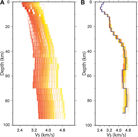
FIGURE 6. (A) Initial 1-D models used for inversion and (B) corresponding inverted 1-D models. Blue line indicates the model chosen for further analysis.
Shear Wave Velocity Structure
Inverted 1D Vs models at all nodes are used to obtain lateral 2D variation (Figure 7, Supplementary Figure S7), and combining these 2D models, 3D velocity structure is obtained. 2D Vs map indicates ∼2.8–3.0 km/s average velocity at 4 km depth in the southern Tibet and Lhasa block. It increases gradually to ∼3.3 km/s at 6 km depth, to ∼3.4–3.6 km/s at 10 km, and ∼3.6–3.8 km/s at 24 km depth. The average velocity values at different depths match well with the 1D velocity results of Monsalve et al. (2008). A low-velocity zone is observed at the mid-crustal level (∼27–50 km) for southern Tibet, which is similar to the observations of Jiang et al. (2011), Sun et al. (2010), and Kumar et al. (2018b; 2019). The ultra-low velocity (∼3.3 km/s) zones in the mid-crust of southern Tibet have been suggested to be due to partial melting or aqueous fluid (Cogan et al., 1998; Makovsky & Klemperer, 1999; Unsworth et al., 2005; Jiang et al., 2014). Low-velocity derived in the present study is supported by previous geophysical studies, for example, observation of low-velocity anomaly (Kind et al., 1996; Hung et al., 2010; Hetényi et al., 2011; Kumar et al., 2019), bright spot (Brown et al., 1996; Makovsky et al., 1996), high electric conductivity (Chen et al., 1996; Wei et al., 2001), magnetotelluric study (Unsworth et al., 2004; Arora et al., 2007), and high heat flow (Francheteau et al., 1984).
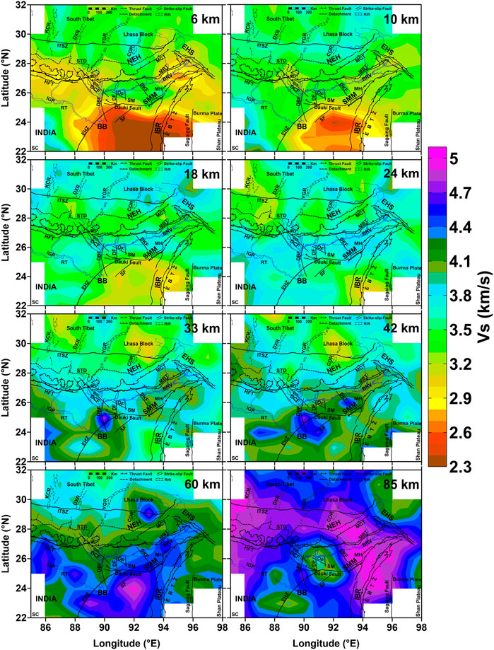
FIGURE 7. Lateral variation of Vs at different depths. Abbreviations of tectonic features are as in Figure 1A.
Part of the Nepal Himalayas (between 85°E–∼88°E) is located within the study area. Top ∼8 km here contains low-velocity material (<2.8 km/s) that has a velocity lower than that in NE Himalayas at the same depth level (Figure 7, Supplementary Figure S7). Down to ∼10 km depth, there is a variation in Vs along the Himalayas from Nepal to NE Himalayas. A positive velocity gradient is observed from 4 to 18 km depth (ranging from ∼2.4 to 2.6 km/s to ∼3.6–3.8 km/s) in the Nepal Himalayas. In NE Himalayas, this value varies from 3.0 to 3.6 km/s in the same depth range. Velocity gradient up to 18 km is relatively higher in the Nepal Himalayas as compared to that in the NE Himalayas and south Tibet (see also Raoof et al., 2017).
In the upper part of the crust down to ∼21 km depth, Vs in BB is low compared to other parts of the study area (Figure 7, Supplementary Figure S7). This contrast is very high for the uppermost crust and distinctly visible between ∼6 and 8 km depth indicating thick sediment depositions in the basin. The margin of low-velocity sediment deposition is demarcated by Dauki fault in the north. Although Vs increases gradually with depth, roots of low-velocity are visible down to ∼21 km depth. Curray et al. (1982) and Brune and Singh (1986) also suggested that sediments/meta-sediments are present down to ∼22 km depth in this region. Variation of sedimentary layer thickness in the BB observed by us is also seen by Singh et al. (2016). We find Vs representative of the crustal basement at depth below ∼24 km. At depth ≥24 km, the Vs below BB is similar to that of oceanic crust (Sowers and Boyd, 2019) The basement also dips in the SE direction.
There are numerous active thrust faults in IBR (Le Dain et al., 1984). Low-velocity up to a depth of ∼10 km is observed below the entire IBR. This could be because of several reasons, viz., presence of cracks, fluid, partial melting, or underthrusting of sediments. However, as Vs in this zone is similar to that observed in the adjacent BB, underthrusting seems most plausible. The low-velocity zone shifts southward along IBR. It is observed down to ∼15–∼18 km depth within the southern part of IBR. Below this depth, the velocity values are representative of crustal material. Therefore, the thickness of sediments below IBR increases from north to south. The high-velocity medium below 50 km depth may represent the subducting lithosphere as proposed by Raoof et al. (2017).
The BB, SMM, and BRV are trapped between two tectonic arcs. There is a very sharp change in velocity across the Dauki fault that separates BB from SMM with a very clear signature from ∼4 to ∼18 km depth (Figure 7, Supplementary Figure S7). This shows that the Dauki fault separates the deep-seated sediments of BB from the crystalline rocks of SMM. Low Vs in the upper ∼4 km in IGP and BRV can be associated with thick sediment deposits (Figure 7, Supplementary Figure S7) (see also Mitra et al., 2006; Suresh et al., 2008; Kumar et al., 2017). It is observed that sedimentary layer thickness varies in the IGP and especially in BRV. Within IGP and NE corner of BRV sedimentary rocks are observed up to 6 km depth, whereas within BRV north of SMM, its thickness is less than 4 km (Figure 7, Supplementary Figure S7).
To get a better perspective about the medium characteristics, S-wave velocity variation along eight profiles (Figure 1A) are presented (Figure 8). Profile AA’ (Figures 1A, 8A) is aligned SSW-NNE which crosses the IGP, Nepal Himalayas, and Tibetan plateau. Prominent tectonic features along this section are HFT, MBT, MCT, STD, and ITSZ. The surface wave is not sensitive to sharp discontinuities like Moho but gives absolute velocity for a depth section across the discontinuity. Kumar et al. (2019) correlated the Rayleigh wave tomography data with the receiver function of the Himalaya–Karakoram–Tibet region to evaluate 4 km/s S-wave contours of tomography results as the approximation of Moho discontinuity. Acton et al. (2010) obtained a 4.1 km/s contour of Moho based on the Rayleigh wave tomography data of the Indian continent and Tibet. Based on the receiver function analysis, Bora et al. (2014) obtained 4 km/s S-wave velocity for Moho in a large part of NE India. In the present study, Moho is marked at 4 km/s (Figure 8). Figure 8A shows that crustal thickness increases gradually from south to north which clearly shows the effect of underthrusting of Indian plate below the Himalayas. In the south beneath IGP, the Moho depth is ∼30 km, which increases to ∼80 km beneath Tibet. In the Nepal Himalayas, interfingering of high- and low-velocity material indicates repeated underthrusting and overthrusting of crustal and mantle material, respectively. Based on the receiver function analysis, Acton et al. (2011) observed imbrication of the crust in the same region. This further supports our observation. A very low-velocity medium north of ITSZ near the Kung-Co rift at a depth range of 30–50 km probably represents a zone of partial melting and/or the presence of aqueous fluid (Makovsky and Klemperer, 1999; Unsworth et al., 2005; Klemperer, 2006). Our observation along this profile is showing good agreement with the finding of the presence of ramp-flat-ramp geometry of the Main Himalayan Thrust (MHT) in the Sikkim Himalaya using joint inversion of receiver functions and surface wave dispersions by Paul and Mitra (2017).
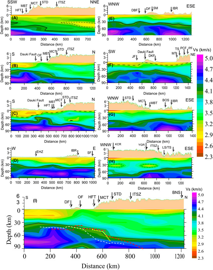
FIGURE 8. (A–I)Vs structure along different profiles marked in Figure 1. Legend: solid line—Moho discontinuity, dashed line—sedimentary layer lower boundary, and dotted line—broken off part of uppermost mantle material (Panel 8G). Dashed lines in Panel 8H encompass low-velocity zones in mid-crust in Lhasa/south Tibet region. (i) Comparison of estimated Moho depth variation along profile BB’ (black line, Panel 8B) with that obtained by Priestley et al. (2008) (white dash line), Mitra et al. (2005) (red dash line), and Singer et al. (2017) (yellow dotted line). Abbreviations: JF: Jamuna fault; MT: Mishmi Thrust; TS: Tidding Suture; PCF: Po Chu fault; PF: Parlung fault; BOS: Belt of Schuppen; SF: Sagaing fault; LT/TS: Lohit Thrust/Tidding Suture, and other abbreviations as in Figure 1A.
Profile BB’ (Figures 1A, 8B) starts from the BB; passes through the SM, NEH, and Lhasa block; and reaches the Bangong–Nujiang Suture (BNS) of south Tibet. The topography is highly variable (minimum and close to mean sea level at BB and BRV). The Moho depth is also highly variable from ∼33 km beneath BB, gradually increasing toward the north up to the frontal Himalayas. Around SM, the crustal thickness is ∼40 km. In the Himalayas from MBT to MCT, the Moho depth suddenly increases and mirrors the increase in topography height. In the Bhutan Himalayas, the Moho depth obtained in this study is similar to that obtained by Singer et al. (2017). Further north, it gradually increases to ∼75 km depth. A very striking result is the low-velocity in the uppermost crust down to ∼20–22 km in the BB for more than 200 km in the southern part. This suggests the presence of thick sediment deposits. The uppermost crustal velocity of SM is higher than that of BB and BRV. The boundary between the sedimentary rock and upper crust (dashed line) clearly shows that the Dauki fault juxtaposes sediments of BB and crystalline rocks of SM. This also suggests that the Massif is either a pop-up structure (Bilham and England, 2001) or the crest of buckled-up Indian plate (Raoof et al., 2017).
Profile CC’ (Figures 1A, 8C) passes through the IBR, SM, MH, NEH, and southern Tibet and shows abnormal Moho depth in the central part of the profile. In the southernmost part, this discontinuity is marked at ∼40 km depth with a gradual increase toward the north for about 300 km passing through IBR. South of Dauki fault, a sudden bend is detected in the Moho discontinuity with a sudden uplift in a localized zone of 200 km beneath MH. This observation is similar to Profile BB’, where the sudden uplift is observed in the boundary between the sedimentary rock layer and the crystalline crust and supports the hypothesis that MH, like SM, is either a pop-up structure or it sits atop the crest of the buckled-up Indian plate. Moho depth is observed between ∼30 and 32 km beneath the MH. Borah et al. (2016) obtained crustal thickness of 32–36 km north of SM based on the S-wave velocity model. The occurrence of thinned crust (30–32 km) beneath SM is also reported by Mitra et al. (2018) and Priestley et al. (2019). The sedimentary layer thickness progressively decreases from IBR to NEH. The low-velocity zone is seen in the mid-to-lower crust beneath Tibet and close to ITSZ that is also visible in Profile HH’ (Figure 8H).
Profile DD’ (Figures 1A, 8D) starts from the west of BB and continues up to the Sagaing fault. An ∼10-km thick layer of sedimentary rocks observed in the western part of BB up to EHZ increases down to ∼20–21 km in the east beneath BB and IBR. Underthrusting of sedimentary wedge below the IBR is observed in both east and west. Moho depth varies between ∼30 and 40 km.
Profile EE’ (Figures 1A, 8E) is along WNW-ESE from the IGP up to IBR. Within BB, low-velocity in the uppermost part is due to the thick sediments. In the west of the IBR, an ∼20–21 km thick pile of sediment is visible. Moho is undulating and its depth is ∼30 km at the WNW end and ∼50 km at the ESE end.
Profile FF’ (Figures 1A, 8F), from the southwest of BB, crosses the BB, passes through SM, a long stretch of BRV, and then perpendicularly traverses the syntaxial bend of EHS. It is the longest section that stretches over 1,450 km and crosses many geological features and tectonic discontinuities. In the BB, it aligns nearly along the strike of EHZ. The profile crosses the Dauki fault to the south of SM and DKF to its northeast. Along the EHS, the section passes through the Mishmi Hills and several NW-SE trending faults. It shows low-velocity in the uppermost crust at both the sides of the SM related to thick sediment deposits of the BB and BRV. In the SM, the sedimentary rock layer thickness is very low. Crustal thickness varies between 35 and 70 km with the thinnest crust beneath the Massif and below the BRV close to the Massif and thickest in the northeast end beneath the EHS. Borah et al. (2016) obtained a crustal thickness of 36–40 km in the Assam valley using the S-wave velocity model. In BB, its value is between 40 and 45 km and decreases toward the northeast. Its thickest geometry in the EHS indicates subduction of the Indian plate. The increase in crustal thickness on either side of the Massif supports the observations of Raoof et al. (2017) suggesting upward crustal buckling beneath the Massif.
Profile GG’ (Figures 1A, 8G) is oblique to the Himalayan arc starting from the central Himalayas, crossing a narrow zone of the BRV, SMM, and further east perpendicular to IBR, then it crosses into the Burma plate. In the uppermost crust within the Himalayas and BRV, low-velocity is related to metasedimentary and sedimentary deposits of the Tethys and BRV, respectively. Borah et al. (2016) observed a 44 km thick crust beneath the lesser Himalayan region. Our result shows that the crustal thickness varies between 45 and 60 km with maximum thickness below the Himalayas.
Profile HH’ (Figures 1A, 8H) covers the Lhasa block and EHS. It starts from south Tibet near the Kung-Co rift, passes through the Yadung-Gulu rift, ITSZ, Mishmi Hills, and ends within the EHS. The topography in southern Tibet is high and the Moho depth is ∼70–75 km for the initial 500 km of the profile. Crustal thickness suddenly decreases near the Yadong-Gulu rift and after that, it gradually decreases to ∼40 km near the EHS. Beneath the Tibetan plateau/Lhasa block, two broad low-velocity zones are detected within ∼30–40 km for a distance of about 300 km. Other workers (Brown et al., 1996; Kind et al., 1996; Nelson et al., 1996; Cogan et al., 1998; Hetényi et al., 2011; Jiang et al., 2014) also observed low-velocity medium in this region.
Priestley et al. (2008) and Mitra et al. (2005) using the receiver function estimated the Moho depth variation along an NS profile starting from 22.60°N and 91.25°E which is close to the profile BB’ of this study (Figure 8B). In Figure 8I, the Moho depth reported by them is superposed on profile BB’. Our estimated Moho depth is shallower in most parts of the profile than their estimates. Although the Moho position estimated by them does not exactly match that of ours, the general trend of Moho depth variation is similar. Beneath the Higher Himalayas, the Moho depth suddenly dips toward north; similar observations are reported by Singer et al. (2017) and Mitra et al. (2005).
Result and Discussion
Bay of Bengal and Indo-Burma Range
The Bay of Bengal is characterized by the thickest sediment deposition in the whole world. Huge sediment deposition occurred in BB during the early-mid Miocene following collision between India and Eurasia (Alam et al., 2003). The large and quick influx of clastic sediments within the basin from the Himalayas in the north and IBR in the east led to sudden subsidence of the basin. At this stage, deep-marine sedimentation at the deeper part of the basin and deep to shallow marine sedimentation in the eastern part of the basin occurred (Alam et al., 2003). Mitra et al. (2018) observed the presence of 18–20 km thick sediment underlain by crystalline crust beneath the central BB. Our results show that sedimentary layer thickness is ∼10 km in the western part of BB and it starts increasing rapidly east of EHZ with a maximum value of ∼21 km at the eastern end of BB (Figures 7, 8, Supplementary Figure S7). The margin of low-velocity sediment deposition is demarcated by the Dauki fault in the north and IBR in the east. Although Vs increases gradually with depth, low-velocity strata are visible down to ∼21 km depth. Thick sediment deposition in the BB camouflages basement configuration and makes it difficult to find the exact location of the boundary between oceanic and continental crusts (Alam et al., 2003). The oceanic crust contains only the mafic rock layer, whereas the continental crust has both the felsic layer overlying the mafic layer. Mafic rocks usually have higher P/S wave velocity than felsic rocks. Also, oceanic crust is thinner than the continental crust. It is observed that the crust underlying the thick sedimentary cover of BB has a thickness varying between ∼10 and 18 km and Vs ∼3.8 km/s (Figures 7, 8B,C, Supplementary Figure S7), which is similar to that of oceanic crust (Gonzalez et al., 2007; Pasyanos and Walter, 2002). North of the Dauki fault, a crustal layer having an S wave velocity similar to that of continental crust (Vs ∼3.4 km/s) overlying this layer is also observed and the total thickness of these two layers increases northward (Data and Estimation of Group Velocity in Figure 7). Hence, north of the Dauki fault crustal structure is similar to the continental crust. Based on these observations, we propose that BB is underlain by oceanic crust, and north of the Dauki fault, the crust is continental (Figures 7, 8B,C, Supplementary Figure S7). Hence, we conclude that the Dauki fault represents an area where the transition of oceanic crust toward its south to continental crust toward its north occurs. Thus, we find clear demarcation between the oceanic and continental crusts. Based on paleomagnetic, gravity, and deep seismic sounding data, Talwani et al. (2016) too found the zone of transition from oceanic to continental crust near this area. Brune and Singh (1986) and Kumar et al. (2018a) found that average Vs in BB changes from oceanic type in its southern part to more continental type toward the north. Based on previous works using Rayleigh wave close to this study region (Acton et al., 2010; Bora et al., 2014; Kumar et al., 2019), 4.0 km/s contour is taken as the Moho discontinuity.
Numerous active thrust faults have been reported in Burma (Le Dain et al., 1984). Low-velocity up to a depth of ∼10 km is observed below the entire IBR. With increasing depth, this low-velocity zone shifts southward along IBR with a gradual increase in velocity. It is observed up to ∼15–∼18 km depth within a very small portion representing the thickness of sediments as they match with velocity observed in the adjacent part of BB (Figures 7, 8, Supplementary Figure S7). Below this depth, the velocity values are representative of crustal material. This shows that the depth up to which sedimentary rocks are present below the IBR increases from north to south. High-velocity medium below 50 km depth in this region may represent the subducting lithosphere (Figures 7, 8, Supplementary Figure S7) as reported by Raoof et al. (2017). Based on local earthquake tomography over a part of the IBR and Burma plate, Zhang et al. (2021) too find evidence of eastward subduction of the India plate below the Burma plate.
Shillong-Mikir Massif, Indo-Gangetic Plain, and Brahmaputra River Valley
Low Vs in the upper ∼4 km in the IGP and BRV is associated with thick sediment deposits. Evaluated Moho depth, based on 4 km/s velocity contour, varies between ∼30 and 40 km (Figures 7, 8). Thick sediments observed by us and highly oblique plate motion suggested by Kayal (2008) between India and IBR suggest the presence of active shallow dipping and locked megathrust faults (Steckler et al., 2016). We find a high Vs structure between ∼50 and ∼75 km (Supplementary Figure S7) within the BB formed due to crustal-scale buckling. At deeper depth, a high-velocity gradient shifted eastward and toward the IBR (Figure 7).
The SMM and BRV are sandwiched between two tectonic arcs where large earthquakes occur. Vs in SMM is representative of high-velocity crystalline rock bodies near the surface, whereas an ∼6 km thick sediment is present in the BRV (Figure 7). A sharp change in velocity across the Dauki fault separating the BB from the SMM is observed, especially between ∼6 and ∼18 km depth. This shows that the Dauki fault separates the deep-seated sediments of BB from the crystalline rocks of SMM, where sediment thickness is negligible. High Vs beneath SMM reveals uplifted crust/uppermost mantle caused by it being in a vice-like grip between the Himalayas and IBR (Figures 1A, 8B,C,F).
It has been suggested that upliftment of SM is caused by N-S compression due to Himalayan collision and E-W directed compression due to the Indo-Burman subduction (Chen and Molnar, 1990; Mukhopadhyay et al., 1997; Rao and Kumar, 1997; Najman et al., 2016; Govin et al., 2018). Upliftment of the SM is linked with kinematic changes in response to a collision between the Himalayas and the Indian plate and subduction of the Indian plate below the Burma plate cumulatively (Clark and Bilham, 2008). The crustal structure of NE India using the P-wave receiver function (Mitra et al., 2018) suggested that the SM uplifted due to thrust faulting on the Dauki fault, continent margin paleo rift fault, and back-thrusting Oldham fault. Strong et al. (2019) stated that the Massif consists of an actively uplifting block with associated continuous erosion processes.
Nepal Himalayas, Northeastern Himalayas, and South Tibet
A variation in Vs along the Himalayas from Nepal to NEH is noted down to a depth of ∼10 km (Figures 7, 8). Velocity values at each of 12–24 km, 33–45 km, and 65–90 km depth range all along this zone are uniform. At other depth ranges, variation in velocity is observed along the trend of the Himalayas. This may be the effect of complex structural geometry in this region. Velocity gradient down to 18 km is relatively higher in the Nepal Himalayas than that in the NEH and south Tibet. Koulakov et al. (2015) estimated that the Moho depth varies both along and across the tectonic trend of the Nepal Himalayas and suggested that the first is due to the crumpling of the crust caused by the stress along the tectonic trend due to counterclockwise rotation of the Indian plate after the first contact with the Asian plate in the NW Himalayas. Observed lateral velocity variation along the tectonic trend in the NE and NW Himalayas (Koulakov et al., 2015; Raoof et al., 2017; Raoof et al., 2018) and our results in this study also support this contention.
Variation in Vs (Figures 7, 8) in southern Tibet and the Lhasa block matches well with the 1D velocity model estimated by Monsalve et al. (2008) for this region. In the mid-crust (∼27–50 km), ultralow-velocity (∼3.3 km/s) zone is observed which is also supported by other researchers using different geophysical studies (Francheteau et al., 1984; Brown et al., 1996; Chen et al., 1996; Kind et al., 1996; Makovsky et al., 1996; Nelson et al., 1996; Wei et al., 2001; Unsworth et al., 2004; Arora et al., 2007; Hung et al., 2010; Jiang et al., 2011). This may indicate partial melting or the presence of aqueous fluid. It is observed that the zones having partial melt/aqueous fluids do not form a continuous layer in southern Tibet but appear rather localized (Figures 7, 8). Hetényi et al. (2011) too observed that zones having partial melts/aqueous fluids are discontinuous in nature.
Eastern Himalayan Syntaxis
EHS is the frontal part of the sandwiched Indian plate between the Eurasian and Burma plate. Sediment thickness of ∼6 km is observed toward the northeast of BRV. An abrupt change in crustal thickness is observed in EHS between the F′ and H′ edges (Figures 1A, 8F,H) of profiles FF′ and HH′, respectively. These two points are on the two sides of EHS, but they are quite close to each other. However, our study shows that the crust is 70 and 45 km thick near the F’ and H’ edges, respectively. Significant variation in crustal thickness within the northeast part of the EHS suggests that the nature of crustal deformation in the EHS is complex. Crustal thickness across the Tidding Suture is 55 km (Hazarika et al., 2012). An increase in crustal thickness within the EHS can be interpreted as an effect of indentation geometry of the Indian plate from the southwest direction. Convergence of Indian and Eurasian plates generates N-S and E-W compression within the NE India, leading to crustal buckling across the NE axis as shown in this work.
Conclusion
a) Bengal Basin is underlain by oceanic crust. Further north below the Shillong Massif/Brahmaputra River Valley, the crust changes to continental type.
b) Thickness of BB sediments increases from west to east. This inference is similar to previous estimates of sediment thickness for this area. The dip of the basement of this sedimentary basin increases suddenly to the east of the Eastern Hinge Zone.
c) Sediments are also getting underthrusted at the southern part of the Indo-Burma Ranges that lie within the study area.
d) In the Indo-Gangetic Plains and Brahmaputra River Valley, 5–6 km thick sedimentary layers are present. This observation is also reported by previous workers. However, north of SMM sedimentary layer is very thin.
e) Across the Dauki fault, low-velocity sediments of Bengal Basin are juxtaposed with high-velocity granitic/metamorphic rocks of the Shillong Massif and Mikir Hills. In the Shillong Massif and Mikir Hills, sedimentary layer cover is very thin or absent and crystalline rocks having higher velocity are present near the surface.
f) Shillong Massif and Mikir Hills lie atop the Indian plate that has buckled up because in this area, the Indian plate is in a vice-like grip between tectonically active Himalayan ranges toward the north, below which it is underthrusting, and the Indo-Burma Ranges toward the east, below which it is subducting (Grujic et al., 2018).
g) The Moho depth varies not only from south to north but also along the tectonic trends of the Himalayas.
h) Average Moho depth increases from ∼40 km in the south to ∼70 km in the northern part of the study area smoothly in most places but abruptly at other places.
i) In the eastern part of the Nepal Himalayas, the signature of repeated underthrusting and overthrusting is observed, whereas such a pattern is not observed further east along the trend of the Himalayas.
j) For southern Tibet/Lhasa block, two important findings are as follows 1) the Moho depth decreases from ∼70 km west of the Yadong-Gulu rift to ∼60 km toward the east which may be the effect of collision geometry to control the underplating of Indian plate in this section of southern Tibet/Lhasa block (Shi et al., 2015); 2) few low-velocity zones are observed in velocity sections at mid-crustal levels near or below the rift zones in the southern Tibet/Lhasa block. This could be due to the presence of zones having partially molten material and/or aqueous fluids. This observation is similar to many seismic and magnetotelluric studies in this area.
Data Availability Statement
The original contributions presented in the study are included in the article/Supplementary Material; further inquiries can be directed to the corresponding author.
Author Contributions
All authors listed have made a substantial, direct, and intellectual contribution to the work and approved it for publication.
Conflict of Interest
The authors declare that the research was conducted in the absence of any commercial or financial relationships that could be construed as a potential conflict of interest.
Publisher’s Note
All claims expressed in this article are solely those of the authors and do not necessarily represent those of their affiliated organizations or those of the publisher, the editors, and the reviewers. Any product that may be evaluated in this article, or claim that may be made by its manufacturer, is not guaranteed or endorsed by the publisher.
Acknowledgments
We are thankful to IMD for providing data. AK is thankful to the Ministry of Human Resource Development, Government of India, for the fellowship through grant #MHR01-23-200-428. AK also acknowledges NCPOR for partial completion of manuscript writing work in the institute through reference no. J-33/2021-22. This research did not receive any specific grant from funding agencies in the public, commercial, or not-for-profit sectors. The authors sincerely acknowledge editor György Hetényi and two reviewers for valuable suggestions for improvement of the manuscript.
Supplementary Material
The Supplementary Material for this article can be found online at: https://www.frontiersin.org/articles/10.3389/feart.2021.680361/full#supplementary-material
References
Acton, C. E., Priestley, K., Gaur, V. K., and Rai, S. S. (2010). Group Velocity Tomography of the Indo-Eurasian Collision Zone. J. Geophys. Res. 115, 1–16. doi:10.1029/2009JB007021
Acton, C. E., Priestley, K., Mitra, S., and Gaur, V. K. (2011). Crustal Structure of the Darjeeling-Sikkim Himalaya and Southern Tibet. Geophys. J. Int. 184, 829–852. doi:10.1111/j.1365-246X.2010.04868.x
Alam, M., Alam, M. M., Curray, J. R., Chowdhury, M. L. R., and Gani, M. R. (2003). An Overview of the Sedimentary Geology of the Bengal Basin in Relation to the Regional Tectonic Framework and basin-fill History. Sediment. Geology. 155, 179–208. doi:10.1016/s0037-0738(02)00180-x
Angelier, J., and Baruah, S. (2009). Seismotectonics in Northeast India: a Stress Analysis of Focal Mechanism Solutions of Earthquakes and its Kinematic Implications. Geophys. J. Int. 178, 303–326. doi:10.1111/j.1365-246X.2009.04107.x
Armijo, R., Tapponnier, P., Mercier, J. L., and Tong-Lin, H. (1986). Quaternary Extension in Southern Tibet: Field Observations and Tectonic Implications. J. Geophys. Res. Solid Earth 91 (13), 803–813. doi:10.1029/jb091ib14p13803872
Arora, B. R., Unsworth, M. J., and Rawat, G. (2007). Deep Resistivity Structure of the Northwest Indian Himalaya and its Tectonic Implications. Geophys. Res. Lett. 34, L04307. doi:10.1029/2006GL029165
Backus, G., and Gilbert, F. (1968). The Resolving Power of Gross Earth Data. Geophys. J. Int. 16, 169–205. doi:10.1111/j.1365-246x.1968.tb00216.x
Baranowski, J., Armbruster, J., Seeber, L., and Molnar, P. (1984). Focal Depths and Fault Plane Solutions of Earthquakes and Active Tectonics of the Himalaya. J. Geophys. Res. 89, 6918–6928. doi:10.1029/jb089ib08p06918
Baruah, S., Baruah, S., and Kayal, J. R. (2013). State of Tectonic Stress in Northeast India and Adjoining South Asia Region: An Appraisal. Bull. Seismological Soc. America 103 (2A), 894–910. doi:10.1785/0120110354
Baruah, S., Baruah, S., Saikia, S., Shrivastava, M. N., Sharma, A., Reddy, C. D., et al. (2016). State of Tectonic Stress in Shillong Plateau of Northeast India. Phys. Chem. Earth, Parts A/B/C 95, 36–49. doi:10.1016/j.pce.2015.11.009
Baruah, S., Saikia, S., Baruah, S., Bora, P. K., Tatevossian, R., and Kayal, J. R. (2014). The September 2011 Sikkim Himalaya Earthquake Mw 6.9: Is it a Plane of Detachment Earthquake? Geomatics, Nat. Hazards Risk 7, 248–263. doi:10.1080/19475705.2014.895963
Bensen, G. D., Ritzwoller, M. H., Barmin, M. P., Levshin, A. L., Lin, F., Moschetti, M. P., et al. (2007). Processing Seismic Ambient Noise Data to Obtain Reliable Broad-Band Surface Wave Dispersion Measurements. Geophys. J. Int. 169, 1239–1260. doi:10.1111/j.1365-246x.2007.03374.x
Bhattacharya, S. N., Mitra, S., and Suresh, G. (2013). The Shear Wave Velocity of the Upper Mantle beneath the Bay of Bengal, Northeast Indian Ocean from Interstation Phase Velocities of Surface Waves. Geophys. J. Int. 193, 1506–1514. doi:10.1093/gji/ggt007
Bilham, R., and England, P. (2001). Plateau 'pop-Up' in the Great 1897 Assam Earthquake. Nature 410, 806–809. doi:10.1038/35071057
Bora, D. K., Hazarika, D., Borah, K., Rai, S. S., and Baruah, S. (2014). Crustal Shear-Wave Velocity Structure beneath Northeast India from Teleseismic Receiver Function Analysis. J. Asian Earth Sci. 90, 1–14. doi:10.1016/j.jseaes.2014.04.005
Borah, K., Bora, D. K., Goyal, A., and Kumar, R. (2016). Crustal Structure beneath Northeast India Inferred from Receiver Function Modeling. Phys. Earth Planet. Interiors 258, 15–27. doi:10.1016/j.pepi.2016.07.005
Brown, L. D., Zhao, W., Nelson, K. D., Hauck, M., Alsdorf, D., Ross, A., et al. (1996). Bright Spots, Structure, and Magmatism in Southern Tibet from INDEPTH Seismic Reflection Profiling. Science 274, 1688–1690. doi:10.1126/science.274.5293.1688
Brune, J. N., Curray, J., Dorman, L., and Raitt, R. (1992). A Proposed Super-thick Sedimentary basin, Bay of Bengal. Geophys. Res. Lett. 19, 565–568. doi:10.1029/91GL0313410.1029/91gl03134
Brune, J. N., and Singh, D. D. (1986). Continent-like Crustal Thickness beneath the Bay of Bengal Sediments. Bull. Seismological Soc. America 76, 191–203. doi:10.1785/bssa0760030903b
Burchfiel, B. C., and Royden, L. H. (1985). North-south Extension within the Convergent Himalayan Region. Geol 13 (10), 679–682. doi:10.1130/0091-7613(1985)13<679:newtch>2.0.co;2
Chen, L., Booker, J. R., Jones, A. G., Wu, N., Unsworth, M. J., Wei, W., et al. (1996). Electrically Conductive Crust in Southern Tibet from INDEPTH Magnetotelluric Surveying. Science 274, 1694–1696. doi:10.1126/science.274.5293.1694
Chen, W.-P., and Molnar, P. (1990). Source Parameters of Earthquakes and Intraplate Deformation beneath the Shillong Plateau and the Northern Indoburman Ranges. J. Geophys. Res. 95, 12527–12552. doi:10.1029/jb095ib08p12527
Clark, M., and Bilham, R. (2008). Miocene Rise of the Shillong Plateau and the Beginning of the End for the Eastern Himalaya. Earth Planet. Sci. Lett. 269, 337–351. doi:10.1016/j.epsl.2008.01.045
Cogan, M. J., Nelson, K. D., Kidd, W. S. F., and Wu, C.Project INDEPTH Team (1998). Shallow Structure of the Yadong-Gulu Rift, Southern Tibet, from Refraction Analysis of Project INDEPTH Common Midpoint Data. Tectonics 17 (1), 46–61. doi:10.1029/97tc03025
Curray, J. R., Emmel, F. J., Moore, D. G., and Raitt, R. W. (1982). “Structure, Tectonics, and Geological History of the Northeastern Indian Ocean,” in The Ocean Basins and Margins (Boston, MA: Springer US), 399–450. doi:10.1007/978-1-4615-8038-6_9
Curray, J. R. (1991). Possible Greenschist Metamorphism at the Base of a 22-km Sedimentary Section, Bay of Bengal. Geol 19, 1097–1100. doi:10.1130/0091-7613(1991)019<1097:pgmatb>2.3.co;2
Curray, J. R. (1989). The Sunda Arc: A Model for Oblique Plate Convergence. Neth. J. Sea Res. 24, 131–140. doi:10.1016/0077-7579(89)90144-0
De Sarkar, S., Mathew, G., and Pande, K. (2013). Arc Parallel Extension in Higher and Lesser Himalayas, Evidence from Western Arunachal Himalaya, India. J. Earth Syst. Sci. 122 (3), 715–727. doi:10.1007/s12040-013-0298-7
DeCelles, P. G., Robinson, D. M., and Zandt, G. (2002). Implications of Shortening in the Himalayan Fold-Thrust belt for Uplift of the Tibetan Plateau. Tectonics 21 (6), 1–25. doi:10.1029/2001tc001322
Desikachar, S. (1974). A Review of the Tectonic and Geological History of Eastern India in Terms of Plate Tectonics Theory. J. Geol. Soc. India 15, 137–149.
Diehl, T., Singer, J., Hetényi, G., Grujic, D., Clinton, J., Giardini, D., et al. GANSSER Working Group (2017). Seismotectonics of Bhutan: Evidence for Segmentation of the Eastern Himalayas and Link to Foreland Deformation. Earth Planet. Sci. Lett. 471, 54–64. doi:10.1016/j.epsl.2017.04.038
Ditmar, P. G., and Yanovskaya, T. B. (1987). A Generalization of the Backus-Gilbert Method for Estimation of Lateral Variations of Surface Wave Velocity (In Russian). Izv.Akad.Nauk Sssir, Fiz. Zemli 6, 30–60.
Dziewonski, A., Bloch, S., and Landisman, M. (1969). A Technique for the Analysis of Transient Seismic Signals. Bull. Seismological Soc. America 59, 427–444. doi:10.1785/bssa0590010427
Dziewonski, A. M., and Anderson, D. L. (1983). Travel Times and Station Corrections for P Waves at Teleseismic Distances. J. Geophys. Res. 88, 3295–3314. doi:10.1029/jb088ib04p03295
England, P., and Bilham, R. (2015). The Shillong Plateau and the Great 1897 Assam Earthquake. Tectonics 34, 1792–1812. doi:10.1002/2015TC003902
England, P., and Houseman, G. (1989). Extension during continental Convergence with Application to the Tibetan Plateau. J. Geophys. Res. 94 (B12), 561–579. doi:10.1029/jb094ib12p17561
Erduran, M., Çakır, Ö., Tezel, T., Şahin, Ş., and Alptekin, Ö. (2007). Anatolian Surface Wave Evaluated at GEOFON Station ISP Isparta, Turkey. Tectonophysics 434, 39–54. doi:10.1016/j.tecto.2007.02.005
Francheteau, J., Jaupart, C., Jie, S. X., Wen-Hua, K., De-Lu, L., Jia-Chi, B., et al. (1984). High Heat Flow in Southern Tibet. Nature 307, 32–36. doi:10.1038/307032a0
Gahalaut, V. K., Kundu, B., Laishram, S. S., Catherine, J., Kumar, A., Singh, M. D., et al. (2013). Aseismic Plate Boundary in the Indo-Burmese Wedge, Northwest Sunda Arc. Geology 41, 235–238. doi:10.1130/g33771.1
González, O. L., Alvarez, L., Guidarelli, M., and Panza, G. F. (2007). Crust and Upper Mantle Structure in the Caribbean Region by Group Velocity Tomography and Regionalization. Pure Appl. Geophys. 164, 1985–2007. doi:10.1007/s00024-007-0259-7
Govin, G., Najman, Y., Copley, A., Millar, I., van der Beek, P., Huyghe, P., et al. (2018). Timing and Mechanism of the Rise of the Shillong Plateau in the Himalayan Foreland. Geology 46 (3), 279–282. doi:10.1130/g39864.1
Grujic, D., Hetényi, G., Cattin, R., Baruah, S., Benoit, A., Drukpa, D., et al. (2018). Stress Transfer and Connectivity between the Bhutan Himalaya and the Shillong Plateau. Tectonophysics 744, 322–332. doi:10.1016/j.tecto.2018.07.018
Gubbins, D. (2004). Time Series Analysis and Inverse Theory for Geophysicist. Cambridge: Cambridge University Press
Guo, Z., Gao, X., Yao, H. J., Li, J., and Wang, W. M. (2009). Midcrustal Low-Velocity Layer beneath the central Himalaya and Southern Tibet Revealed by Ambient Noise Array Tomography. Geochem. Geophys. Geosystems 10 (5), Q05007. doi:10.1029/2009gc002458
Hazarika, D., Arora, B. R., and Bora, C. (2012). Crustal Structure and Deformation in the Northeast India-Asia Collision Zone: Constraints from Receiver Function Analysis. Geophys. J. Int. 188, 737–749. doi:10.1111/j.1365-246x.2011.05267.x
Herrmann, R. B., and Ammon, C. J. (2002). Computer Programs in Seismology-3.30, Surface Waves, Receiver Functions and Crustal Structure. Available at: http://www.eas.slu.edu/eqc/eqccps.html
Herrmann, R. B. (2013). Computer Programs in Seismology: An Evolving Tool for Instruction and Research. Seismological Res. Lett. 84, 1081–1088. doi:10.1785/0220110096
Herrmann, R. B. (1973). Some Aspects of Band-Pass Filtering of Surface Waves. Bull. Seismological Soc. America 63, 663–671.
Hetényi, G., Vergne, J., Bollinger, L., and Cattin, R. (2011). Discontinuous Low-Velocity Zones in Southern Tibet Question the Viability of the Channel Flow Model. Geol. Soc. Lond. Spec. Publications 353, 99–108. doi:10.1144/sp353.6
Hintersberger, E., Thiede, R. C., Strecker, M. R., and Hacker, B. R. (2010). East-west Extension in the NW Indian Himalaya. Geol. Soc. America Bull. 122, 1499–1515. doi:10.1130/b26589.1
Holt, W. E., Ni, J. F., Wallace, T. C., and Haines, A. J. (1991). The Active Tectonics of the Eastern Himalayan Syntaxis and Surrounding Regions. J. Geophys. Res. 96 (14), 14595–14632. doi:10.1029/91jb01021632
Hung, S.-H., Chen, W.-P., Chiao, L.-Y., and Tseng, T.-L. (2010). First Multi-Scale, Finite-Frequency Tomography Illuminates 3-D Anatomy of the Tibetan Plateau. Geophys. Res. Lett. 37, a–n. doi:10.1029/2009GL041875
Jiang, M., Ai, Y., Zhou, S., and Chen, Y. J. (2014). Distribution of the Low Velocity Bulk in the Middle-To-Lower Crust of Southern Tibet: Implications for Formation of the north-south Trending Rift Zones. Earthq Sci. 27 (2), 149–157. doi:10.1007/s11589-014-0080-1
Jiang, M., Zhou, S., Sandvol, E., Chen, X., Liang, X., Chen, Y. J., et al. (2011). 3-D Lithospheric Structure beneath Southern Tibet from Rayleigh-Wave Tomography with a 2-D Seismic Array. Geophys. J. Int. 185, 593–608. doi:10.1111/j.1365-246x.2011.04979.x
Kailasam, L. N. (1979). Plateau Uplift in Peninsular India. Tectonophysics 61, 243–269. doi:10.1016/0040-1951(79)90300-7
Karagianni, E. E., Panagiotopoulos, D. G., Panza, G. F., Suhadolc, P., Papazachos, C. B., Papazachos, B. C., et al. (2002). Rayleigh Wave Group Velocity Tomography in the Aegean Area. Tectonophysics 358, 187–209. doi:10.1016/s0040-1951(02)00424-9
Kayal, J. R. (2001). Microearthquake Activity in Some Parts of the Himalaya and the Tectonic Model. Tectonophysics 339, 331–351. doi:10.1016/s0040-1951(01)00129-9
Kayal, J. R. (1996). Precursor Seismicity, Foreshocks and Aftershocks of the Uttarkashi Earthquake of October 20, 1991 at Garhwal Himalaya. Tectonophysics 263, 339–345. doi:10.1016/S0040-1951(97)81488-6
Kayal, J. R. (1989). Subduction Structure at the India/Burma Plate Boundary: Seismic and Gravity Evidences, 2. USA: 28th International Geological Congress, 164–165.
Khattri, K. N., Chander, R., Mukhopadhyay, S., Sriram, V., and Khanal, K. N. (1992). “A Model of Active Tectonics in the Shillong Massif Region,” in The Himalayan Orogen and Global Tectonics. Editor A. K. Sinha (Delhi: Oxford and IBH), 205–222.
Kind, R., Ni, J., Zhao, W., Wu, J., Yuan, X., Zhao, L., et al. (1996). Evidence from Earthquake Data for a Partially Molten Crustal Layer in Southern Tibet. Science 274, 1692–1694. doi:10.1126/science.274.5293.1692
Klemperer, S. L. (2006). Crustal Flow in Tibet: Geophysical Evidence for the Physical State of Tibetan Lithosphere, and Inferred Patterns of Active Flow. Geol. Soc. Lond. Spec. Publications 268 (1), 39–70. doi:10.1144/gsl.sp.2006.268.01.03
Kolinsky, P. (2004). Surface Wave Dispersion Curves of Eurasian Earthquakes: the SVAL Program. Acta Geodynamica Geomaterialia 1 (134), 165–185.
Koulakov, I., Maksotova, G., Mukhopadhyay, S., Raoof, J., Kayal, J. R., Jakovlev, A., et al. (2015). Variations of the Crustal Thickness in Nepal Himalayas Based on Tomographic Inversion of Regional Earthquake Data. Solid Earth 6 (1), 207–216. doi:10.5194/se-6-207-2015
Kumar, A., Kumar, N., Mukhopadhyay, S., and Baidya, P. R. (2017). Crustal and Uppermost Mantle Structures in the Frontal Himalaya and Indo-Gangetic basin Using Surface Wave: Tectonic Implications. Quat. Int. 462, 34–49. doi:10.1016/j.quaint.2017.02.035
Kumar, A., Kumar, N., and Mukhopadhyay, S. (2018b). Investigation of Azimuthal Variation in Seismic Surface Waves Group Velocity in the Western Part of Himalaya-Tibet Indo-Gangetic plains Region. Himalayan Geology. 39 (1), 33–46. doi:10.1111/1755-6724.13931
Kumar, A., Mitra, S., and Suresh, G. (2015). Seismotectonics of the Eastern Himalayan and Indo-Burman Plate Boundary Systems. Tectonics 34, 2279–2295. doi:10.1002/2015tc003979
Kumar, A., Mukhopadhyay, S., Kumar, N., and Baidya, P. R. (2018a). Lateral Variation in Crustal and Mantle Structure in Bay of Bengal Based on Surface Wave Data. J. Geodynamics 113, 32–42. doi:10.1016/j.jog.2017.11.006
Kumar, N., Aoudia, A., Guidarelli, M., Babu, V. G., Hazarika, D., and Yadav, D. K. (2019). Delineation of Lithosphere Structure and Characterization of the Moho Geometry under the Himalaya-Karakoram-Tibet Collision Zone Using Surface-Wave Tomography. Geol. Soc. Lond. Spec. Publications 481, 19–40. doi:10.1144/SP481-2017-172
Le Dain, A. Y., Tapponnier, P., and Molnar, P. (1984). Active Faulting and Tectonics of Burma and Surrounding Regions. J. Geophys. Res. 89 (B1), 453–472. doi:10.1029/JB089iB01p00453
Le Roux-Mallouf, R., Ferry, M., Cattin, R., Ritz, J.-F., Drukpa, D., and Pelgay, P. (2020). A 2600-Year-Long Paleoseismic Record for the Himalayan Main Frontal Thrust (Western Bhutan). Solid Earth 11, 2359–2375. doi:10.5194/se-11-2359-2020
Levshin, A. L., Yanovskaya, T. B., Lander, A. V., Bukchin, B. G., Barmin, M. P., Ratnikova, L. I., et al. (1989). “Recording, Identification, and Measurement of Surface Wave Parameters,” in Seismic Surface Waves in a Laterally Inhomogeneous Earth. Editor V. I. Keilis-Borok (Dordrecht: Kluwer Academic Publisher), 131–182
Makovsky, Y., and Klemperer, S. L. (1999). Measuring the Seismic Properties of Tibetan Bright Spots: Evidence for Free Aqueous Fluids in the Tibetan Middle Crust. J. Geophys. Res. 104 (B5), 10795–10825. doi:10.1029/1998jb900074
Makovsky, Y., Klemperer, S. L., Ratschbacher, L., Brown, L. D., Li, M., Zhao, W., et al. (1996). INDEPTH Wide-Angle Reflection Observation of P-Wave-To-S-Wave Conversion from Crustal Bright Spots in Tibet. Science 274, 1690–1691. doi:10.1126/science.274.5293.1690
Mitchell, A. H. G., and McKerrow, W. S. (1975). Analogous Evolution of the Burma Orogen and the Scottish Caledonides. Geol. Soc. America Bull. 86, 305–315. doi:10.1130/0016-7606(1975)86<305:aeotbo>2.0.co;2
Mitra, S., Kainkaryam, S. M., Padhi, A., Rai, S. S., and Bhattacharya, S. N. (2011). The Himalayan Foreland basin Crust and Upper Mantle. Phys. Earth Planet. Interiors 184, 34–40. doi:10.1016/j.pepi.2010.10.009
Mitra, S., Priestley, K., Bhattacharyya, A. J., and Gaur, V. K. (2005). Crustal Structure and Earthquake Focal Depths beneath north Eastern India and Southern Tibet. Geophys. J. Int. 160, 227–248.
Mitra, S., Priestley, K. F., Borah, K., and Gaur, V. K. (2018). Crustal Structure and Evolution of the Eastern Himalayan Plate Boundary System, Northeast India. J. Geophys. Res. Solid Earth 123, 621–640. doi:10.1002/2017JB014714
Mitra, S., Priestley, K., Gaur, V. K., Rai, S. S., and Haines, J. (2006). Variation of Rayleigh Wave Group Velocity Dispersion and Seismic Heterogeneity of the Indian Crust and Uppermost Mantle. Geophys. J. Int. 164, 88–98. doi:10.1111/j.1365-246X.2005.02837.x
Molnar, P., Chen, W., Fitch, W., Tapponnier, P., Warsi, W., and Wu, F. T. (1977). Structure and Tectonics of the Himalaya: A Brief Summary of Relevant Geophysical Observations. Ecologieet Geologie de l'Himalaya, Colloques internationaux du C.N.R.S. 268, 269–294.
Molnar, P. (1984). Structure and Tectonics of the Himalaya: Constraints and Implications of Geophysical Data. Annu. Rev. Earth Planet. Sci. 12, 489–516. doi:10.1146/annurev.ea.12.050184.002421
Monsalve, G., Sheehan, A., Rowe, C., and Rajaure, S. (2008). Seismic Structure of the Crust and the Upper Mantle beneath the Himalayas: Evidence for Eclogitization of Lower Crustal Rocks in the Indian Plate. J. Geophys. Res. 113, B08315. doi:10.1029/2007JB005424
Motazedian, D., and Ma, S. (2014). Crustal Shear-Wave Velocity Models Retrieved from Rayleigh-Wave Dispersion Data in Northern Canada. Bull. Seismological Soc. America, early edition 104 (4), 1–13. doi:10.1785/0120130265
Mukhopadhyay, M., and Dasgupta, S. (1988). Deep Structure and Tectonics of the Burmese Arc: Constraints from Earthquake and Gravity Data. Tectonophysics 149, 299–322. doi:10.1016/0040-1951(88)90180-1
Mukhopadhyay, S., Chander, R., and Khattri, K. N. (1997). Crustal Properties in the Epicentral Tract of the Great 1897 Assam Earthquake, Northeastern India. Tectonophysics 283, 311–330. doi:10.1016/s0040-1951(97)00148-0
Mukhopadhyay, S., Chander, R., and Khattri, K. N. (1993). Fine Structure of Seismotectonics in Western Shillong Massif, north east India. Proc. Indian Acad. Sci. - Earth Planet. Sci. 102 (2), 383–398.
Murphy, M. A., and Copeland, P. (2005). Transtensional Deformation in the central Himalaya and its Role in Accommodating Growth of the Himalayan Orogen. Tectonics 24, a–n. doi:10.1029/2004TC001659
Nabelek, J., Hetényi, G., Vergne, J., Sapkota, S., Kafle, B., Jiang, M., et al. the Hi-CLIMB Team (2009). Underplating in the Himalaya-Tibet Collision Zone Revealed by the Hi-CLIMB Experiment. Science 325, 1371–1374. doi:10.1126/science.1167719
Najman, Y., Bracciali, L., Parrish, R. R., Chisty, E., and Copley, A. (2016). Evolving Strain Partitioning in the Eastern Himalaya: The Growth of the Shillong Plateau. Earth Planet. Sci. Lett. 433, 1–9. doi:10.1016/j.epsl.2015.10.017
Nelson, K. D., Zhao, W., Brown, L. D., Kuo, J., Che, J., Liu, X., et al. (1996). Partially Molten Middle Crust beneath Southern Tibet: Synthesis of Project INDEPTH Results. Science 274, 1684–1688. doi:10.1126/science.274.5293.1684
Ni, J., and Barazangi, M. (1984). Seismotectonics of the Himalayan Collision Zone: Geometry of the Underthrusting Indian Plate beneath the Himalaya. J. Geophys. Res. 89 (B2), 1147–1163. doi:10.1029/JB089iB02p01147
Ni, J. F., Guzman-Speziale, M., Bevis, M., Holt, W. E., Wallace, T. C., and Seager, W. (1989). Accretionary Tectonics of Burma and the Three Dimensional Geometry of the Burma Subduction Zone. Geol. Soc. America 17, 68–71. doi:10.1130/0091-7613(1989)017<0068:ATOBAT>2.3.CO;2
Oldham, R. D. (1899). Report on the Great Earthquake of 12th June 1897, Mere. Geol. Surv. India 29, 1–379.
Pandey, M. R., Tandukar, R. P., Avouac, J. P., Lavé, J., and Massot, J. P. (1995). Interseismic Strain Accumulation on the Himalayan Crustal Ramp (Nepal). Geophys. Res. Lett. 22, 751–754. doi:10.1029/94gl02971
Parvez, I. A., and Ram, A. (1997). Probabilistic Assessment of Earthquake Hazards in the North-East Indian Peninsula and Hindukush Regions. Pure Appl. Geophys. 149, 731–746. doi:10.1007/s000240050049
Pasyanos, M. E., and Walter, W. R. (2002). Crust and Upper-Mantle Structure of North Africa, Europe and the Middle East from Inversion of Surface Waves. Geophys. J. Int. 149, 463–481. doi:10.1046/j.1365-246x.2002.01663.x
Paul, H., and Mitra, S. (2017). Three-dimensional Crustal Architecture beneath the Sikkim Himalaya and its Relationship to Active Deformation. J. Geophys. Res. Solid Earth 122, 7860–7878. doi:10.1002/2017JB014506
GSI (2000). “Seismotectonic Atlas of India and its Environs,” in Geological Survey of India, Special Publication. Editors P. L. Narula, S. K. Acharya, and P. Banerjee, 86.
Priestley, K., Ho, T., and Mitra, S. (2019). The Crustal Structure of the Himalaya: A Synthesis. Geol. Soc. Lond. Spec. Publications 483, 483–516. doi:10.1144/SP483-2018-127
Priestley, K., Jackson, J., and McKenzie, D. (2008). Lithospheric Structure and Deep Earthquakes beneath India, the Himalaya and Southern Tibet. Geophys. J. Int. 172, 345–362. doi:10.1111/j.1365-246x.2007.03636.x
Rao, N. P., and Kumar, M. R. (1997). Uplift and Tectonics of the Shillong Plateau, Northeast India. J,Phys,Earth 45, 167–176. doi:10.4294/jpe1952.45.167
Raoof, J., Mukhopadhyay, S., Koulakov, I., and Kayal, J. R. (2017). 3-D Seismic Tomography of the Lithosphere and its Geodynamic Implications beneath the Northeast India Region. Tectonics 36, 962–980. doi:10.1002/2016TC004375
Raoof, J., Mukhopadhyay, S., and Malik, J. N. (2018). “3-D Seismic Tomography of the Indo-Asian Collision Zone from Pamir-Hindu Kush in the West to Indo-Burma Ranges in the East: Geodynamic Implications,” in AGU Fall Meeting, Washington DC, USA, Dec 10–14, 2018.
Ritzwoller, M. H., and Levshin, A. L. (1998). Eurasian Surface Wave Tomography: Group Velocities. J. Geophys. Res. 103 (B3), 4839–4878. doi:10.1029/97jb02622
Ritzwoller, M. H., Levshin, A. L., Ratnikova, L. I., and Egorkin, A. A. (1998). Intermediate Period Group Velocity Maps across central Asia, Western China and Parts of Middle-East. Geophys. J. Int. 134, 315–328.
Satyabala, S. P. (2003). Oblique Plate Convergence in the Indo-Burma (Myanmar) Subduction Region. Pure Appl. Geophys. 160, 1611–1650. doi:10.1007/s00024-003-2378-0
Shi, D., Wu, Z., Klemperer, S. L., Zhao, W., Xue, G., and Su, H. (2015). Receiver Function Imaging of Crustal Suture, Steep Subduction, and Mantle Wedge in the Eastern India-Tibet continental Collision Zone. Earth Planet. Sci. Lett. 414, 6–15. doi:10.1016/j.epsl.2014.12.055
Singer, J., Kissling, E., Diehl, T., and Hetényi, G. (2017). The Underthrusting Indian Crust and its Role in Collision Dynamics of the Eastern Himalaya in Bhutan: Insights from Receiver Function Imaging. J. Geophys. Res. Solid Earth 122, 1152–1178. doi:10.1002/2016JB013337
Singh, A., Bhushan, K., Singh, C., Steckler, M. S., Akhter, S. H., Seeber, L., et al. (2016). Crustal Structure and Tectonics of Bangladesh: New Constraints from Inversion of Receiver Functions. Tectonophysics 680, 99–112. doi:10.1016/j.tecto.2016.04.046
Singh, A., Singh, C., and Kennett, B. L. N. (2015). A Review of Crust and Upper Mantle Structure beneath the Indian Subcontinent. Tectonophysics 644-645, 1–21. doi:10.1016/j.tecto.2015.01.007
Sowers, T., and Boyd, O. S. (2019). Petrologic and Mineral Physics Database for Use with the U.S. Geological Survey National Crustal Model. Reston, VA: USGS Open File Report, 2019–1035
Steckler, M. S., Mondal, D. R., Akhter, S. H., Seeber, L., Feng, L., Gale, J., et al. (2016). Locked and Loading Megathrust Linked to Active Subduction beneath the Indo-Burman Ranges. Nat. Geosci 9, 615–618. doi:10.1038/ngeo2760
Strong, C. M., Attal, M., Mudd, S. M., and Sinclair, H. D. (2019). Lithological Control on the Geomorphic Evolution of the Shillong Plateau in Northeast India. Geomorphology 330, 133–150. doi:10.1016/j.geomorph.2019.01.016
Sun, X., Song, X., Zheng, S., Yang, Y., and Ritzwoller, M. H. (2010). Three Dimensional Shear Wave Velocity Structure of the Crust and Upper Mantle beneath China from Ambient Noise Surface Wave Tomography. Earthq Sci. 23, 449–463. doi:10.1007/s11589-010-0744-4
Suresh, G., Jain, S., and Bhattacharya, S. N. (2008). Lithosphere of Indus Block in the Northwest Indian Subcontinent through Genetic Algorithm Inversion of Surface-Wave Dispersion. Bull. Seismological Soc. America 98, 1750–1755. doi:10.1785/0120070254
Talwani, M., Desa, M. A., Ismaiel, M., and Sree Krishna, K. (2016). The Tectonic Origin of the Bay of Bengal and Bangladesh. J. Geophys. Res. Solid Earth 121, 4836–4851. doi:10.1002/2015JB012734
Tapponnier, P., Xu, Z. Q., Roger, F., Meyer, B., Arnaud, N., Wittlinger, G., et al. (2001). Oblique Stepwise Rise and Growth of the Tibet Plateau. Science 294, 1671–1677. doi:10.1126/science.105978
Thiede, R. C., Arrowsmith, J. R., Bookhagen, B., McWilliams, M., Sobel, E. R., and Strecker, M. R. (2006). Dome Formation and Extension in the Tethyan Himalaya, Leo Pargil, Northwest India. Geol. Soc. America Bull. 118, 635–650. doi:10.1130/b25872.1
Unsworth, M. J., Jones, A. G., Jones, A. G., Wei, W., Marquis, G., Gokarn, S. G., et al. (2005). Crustal Rheology of the Himalaya and Southern Tibet Inferred from Magnetotelluric Data. Nature 438, 78–81. doi:10.1038/nature0415410.1038/nature04154
Unsworth, M., Wenbo, W., Jones, A. G., Li, S., Bedrosian, P., Booker, J., et al. (2004). Crustal and Upper Mantle Structure of Northern Tibet Imaged with Magnetotelluric Data. J. Geophys. Res. 109, B02403. doi:10.1029/2002JB002305
Verma, R. K., and Mukhopadhyay, M. (1977). An Analysis of the Gravity Field in Northeastern India. Tectonophysics 42, 283–317. doi:10.1016/0040-1951(77)90171-8
Wei, W., Unsworth, M., Jones, A., Booker, J., Tan, H., Nelson, D., et al. (2001). Detection of Widespread Fluids in the Tibetan Crust by Magnetotelluric Studies. Science 292, 716–719. doi:10.1126/science.1010580
Yang, Y., Ritzwoller, M. H., Levshin, A. L., and Shapiro, N. M. (2007). Ambient Noise Rayleigh Wave Tomography across Europe. Geophys. J. Int. 168, 259–274. doi:10.1111/j.1365-246x.2006.03203.x
Yanovskaya, T. B., and Ditmar, P. G. (1990). Smoothness Criteria in Surface Wave Tomography. Geophys. J. Int. 102, 63–72. doi:10.1111/j.1365-246x.1990.tb00530.x
Yanovskaya, T. B., Kizima, E. S., and Antonova, L. M. (1998). Structure of the Crust in the Black Sea and Adjoining Regions from Surface Wave Data. J. Seismology 2, 303–316. doi:10.1023/A:1009716017960
Yanovskaya, T. B., and Kozhevnikov, V. M. (2003). 3D S-Wave Velocity Pattern in the Upper Mantle beneath the Continent of Asia from Rayleigh Wave Data. Phys. Earth Planet. Interiors 138, 263–278. doi:10.1016/S0031-9201(03)00154-7
Yanovskaya, T. B. (1997). Resolution Estimation in the Problems of Seismic ray Tomography. Izvestia, Phys. Solid Earth 33 (9), 762–765.
Yao, H., Van Der Hilst, R. D., and De Hoop, M. V. (2006). Surface-wave Array Tomography in SE Tibet from Ambient Seismic Noise and Two-Station Analysis - I. Phase Velocity Maps. Geophys. J. Int. 166, 732–744. doi:10.1111/j.1365-246x.2006.03028.x
Keywords: NE India, surface wave, group velocity, tomography, Vs
Citation: Kumar A, Kumar N, Mukhopadhyay S and Klemperer SL (2021) Tomographic Image of Shear Wave Structure of NE India Based on Analysis of Rayleigh Wave Data. Front. Earth Sci. 9:680361. doi: 10.3389/feart.2021.680361
Received: 14 March 2021; Accepted: 16 August 2021;
Published: 08 October 2021.
Edited by:
György Hetényi, University of Lausanne, SwitzerlandReviewed by:
Emanuel David Kästle, Freie Universität Berlin, GermanyBernhard Maximilian Steinberger, German Research Centre for Geosciences, Germany
Copyright © 2021 Kumar, Kumar, Mukhopadhyay and Klemperer. This is an open-access article distributed under the terms of the Creative Commons Attribution License (CC BY). The use, distribution or reproduction in other forums is permitted, provided the original author(s) and the copyright owner(s) are credited and that the original publication in this journal is cited, in accordance with accepted academic practice. No use, distribution or reproduction is permitted which does not comply with these terms.
*Correspondence: Sagarika Mukhopadhyay, c2FnYXJmZXNAZ21haWwuY29t