 Frederik Link
 Georg Rümpker
95% of researchers rate our articles as excellent or good
Learn more about the work of our research integrity team to safeguard the quality of each article we publish.
Find out more
ORIGINAL RESEARCH article
Front. Earth Sci. , 03 September 2021
Sec. Solid Earth Geophysics
Volume 9 - 2021 | https://doi.org/10.3389/feart.2021.679887
This article is part of the Research Topic Mountain Building View all 14 articles
The Alpine orogeny is characterized by tectonic sequences of subduction and collision accompanied by break-off events and possibly preceded by a flip of subduction polarity. The tectonic evolution of the transition to the Eastern Alps has thus been under debate. The dense SWATH-D seismic network as a complementary experiment to the AlpArray seismic network provides unprecedented lateral resolution to address this ongoing discussion. We analyze the shear-wave splitting of this data set including stations of the AlpArray backbone in the region to obtain new insights into the deformation at depth from seismic anisotropy. Previous studies indicate two-layer anisotropy in the Eastern Alps. This is supported by the azimuthal pattern of the measured fast axis direction across all analyzed stations. However, the temporary character of the deployment requires a joint analysis of multiple stations to increase the number of events adding complementary information of the anisotropic properties of the mantle. We, therefore, perform a cluster analysis based on a correlation of energy tensors between all stations. The energy tensors are assembled from the remaining transverse energy after the trial correction of the splitting effect from two consecutive anisotropic layers. This leads to two main groups of different two-layer properties, separated approximately at 13°E. We identify a layer with a constant fast axis direction (measured clockwise with respect to north) of about 60° over the whole area, with a possible dip from west to east. The lower layer in the west shows N–S fast direction and the upper layer in the east shows a fast axis of about 115°. We propose two likely scenarios, both accompanied by a slab break-off in the eastern part. The continuous layer can either be interpreted as frozen-in anisotropy with a lithospheric origin or as an asthenospheric flow evading the retreat of the European slab that would precede the break-off event. In both scenarios, the upper layer in the east is a result of a flow through the gap formed in the slab break-off. The N–S direction can be interpreted as an asthenospheric flow driven by the retreating European slab but might also result from a deep-reaching fault-related anisotropy.
The development of seismic anisotropy is significantly affected by tectonic processes and the dynamics of the Earth’s interior (Savage 1999). The lithosphere and the asthenosphere are the dominant source regions of seismic anisotropy in the crust and upper mantle. In the crust, anisotropy results from the stress-induced alignment of cracks (Christensen, 1966; Nur and Simmons, 1969; Nur, 1971; Crampin 1987; Yousef and Angus 2016) in alternating layers of different seismic velocities like folded sediments (Backus 1962; Savage 1999) or (in the lower crust) an alignment of intrinsically anisotropic minerals. The latter also occurs in the upper mantle lithosphere as frozen-in anisotropy. In the asthenosphere, seismic anisotropy is dominated by the lattice-preferred orientation of olivine crystals that align along the strain direction (Silver 1996; Karato et al., 2008), in response to mantle flow processes (Long and Becker 2010). The most robust observable for measuring seismic anisotropy is the splitting of shear waves, which is commonly inferred from core–mantle converted phases (Silver and Chan 1991; Savage 1999). Shear-wave splitting characterizes anisotropy by a fast axis, which is parallel to the preferred orientation of the mantle minerals in a simple mantle flow–dominated anisotropic model, and a lag time, which scales with the strength of anisotropy and the extent of the anisotropic volume. However, the diverse tectonic history and complex present-day dynamics influence the anisotropy of the upper mantle and lithosphere. Also, large or local shear faults may produce an extended crustal and lithospheric anisotropy above an asthenospheric mantle flow (e.g., Savage 1999; Reiss et al., 2016; Reiss et al., 2018). Lithospheric fragments of subducted slabs can carry frozen-in anisotropy. They result in a pronounced layered anisotropy when they sink (after possible break-off) into the mantle, due to a replacement flow of asthenospheric mantle material (Qorbani et al., 2015a).
The Alpine orogeny is a result of an ensemble of subduction, extension, and collision sequences driven by the convergence of the African and Eurasian plates (Dewey et al., 1973; Dewey et al., 1989; Handy et al., 2010). Prior to the collision of the Adriatic–African and European plates at around 35 Ma, Alpine Tethys and the distal European margin subducted during the convergence initiated at 84 Ma with Adria as the upper plate (Schmid et al., 2004; Handy et al., 2010). With the collision, the Adriatic plate was pushed by the African plate deep into Europe, which led to the formation of a complicated subduction geometry (Handy et al., 2010; Király et al., 2018). Concurrently, a slab break-off was initiated after the completed subduction of the Tethyan units and separated the crustal European units from the subducted lithosphere below the Eastern Alps (von Blanckenburg and Davies, 1995; Lippitsch, 2003; Harangi et al., 2006; Kissling et al., 2006). This was possibly accompanied or preceded by a subduction polarity switch (Schmid et al., 2004; Vignaroli et al., 2008; Handy et al., 2010; Molli and Malavieille 2011; Handy et al., 2015). Especially the subduction polarity below the Eastern Alps is under debate (Kästle et al., 2020), as tomographic studies indicate a northward dip of a possibly Adriatic subduction below Europe (Schmid et al., 2004; Ustaszewski et al., 2008; Schmid et al., 2013), which might be a result of a polarity switch accompanied by a break-off of the previously subducted European slab (Handy et al., 2010; Schmid et al., 2013). For further detailed descriptions of possible models, we refer to the study by Kästle et al. (2020). The present-day tectonic structure can be identified as accreted European units in the Central and Eastern Alps, partially showing metamorphism from deep subduction (Froitzheim et al., 1996; Handy et al., 2010, see also Figure 1). This is separated from the Southern Alps, consisting of Adriatic units by the Tonale Fault (TF) and the Periadriatic Fault (PAF). The main irregularity of the orogen parallel E–W trending faults arises by the Giudicarie Fault (GF), which formed during the indentation of the Adriatic microplate (Handy et al., 2015).
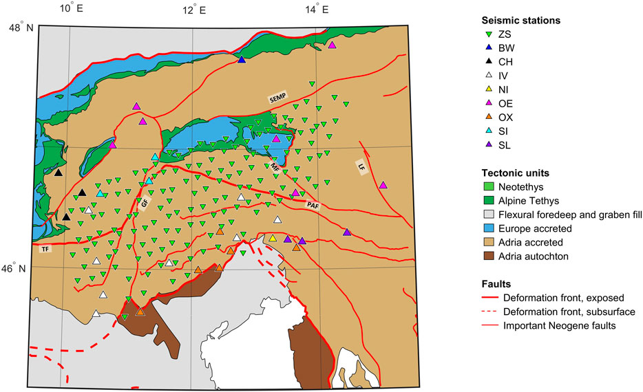
FIGURE 1. Station distribution of the dense SWATH-D complementary seismic network (ZS) and permanent stations of national networks in the same region. Major faults are GF, Giudicarie Fault; PAF, Periadriatic Fault; TF, Tonale Fault; SEMP, Salzach–Ennstal–Mariazell–Puchberg fault system; MF, Mölltal Fault; and LF, Lavanttal Fault. The background shows the geological map compiled by M.R. Handy with units and major lineaments simplified from the works of Bigi et al. (1992), Froitzheim et al. (1996), Schmid et al. (2004), Schmid et al. (2008), Handy et al. (2010), Bousquet et al. (2012), Handy et al. (2015), and Handy et al. (2019).
To address the question of subduction polarity and tectonic evolution in the transition of the Central to the Eastern Alps, the recently established seismic network SWATH-D provides a unique opportunity due to its unprecedented dense station coverage (AlpArray Seismic Network, 2015; Heit et al., 2017; Hetényi et al., 2018a). The 154 stations cover the critical transition between the TRANSALP (Lüschen et al., 2004) and the EASI experiment (Hetényi et al., 2018b) along the Periadriatic Fault (Handy et al., 2010). While the Moho geometry in the TRANSALP experiment was still unclear (Lüschen et al., 2004), the EASI experiment seems to image the Adriatic Moho below the European plate, which indicates an Adriatic subduction (Hetényi et al., 2018b; Kästle et al., 2020). While tomographic studies lack evidence for the subduction polarity in the Eastern Alps (Kästle et al., 2020 and references therein), they clearly suggest a European subduction in the Western and in the Central Alps (Lippitsch, 2003; Zhao et al., 2016). The result from EASI therefore indicates a polarity switch, possibly in the area covered by the SWATH-D complementary network. The present study addresses open questions regarding the slab break-off, slab geometry, and tectonic evolution in this key area of the Alpine system by analyzing the splitting of core–mantle phases due to seismic anisotropy beneath the network. Based on the findings from previous studies and our individual splitting measurements, we specifically account for two-layer anisotropic models which can account for both frozen-in lithospheric and asthenospheric mantle flows, or a present-day two-layer flow in the asthenosphere.
When a shear wave propagates through an anisotropic medium, the wave is split into a fast and a slow phase polarized perpendicular to each other (Savage 1999). The polarization directions coincide with the horizontal projection of the fast and slow directions of the anisotropic medium. Usually, core–mantle converted phases (e.g., SKS, SKKS, PKS, and PKKS) are used for the analysis, as their initial polarization is determined by the event-station geometry, when they leave the Earth’s core. Assuming a radially symmetric isotropic Earth, no splitting occurs, and the initial polarization in the radial direction is preserved in the recording at the receiver. In contrast, after the propagation through an anisotropic medium, seismic energy may be present on the transverse component due to shear-wave splitting. This anisotropic effect can be investigated by applying an inverse splitting operator with the aim to remove the splitting from the recorded data (Silver and Chan 1991). Here, we use the SplitRacer toolbox (Reiss and Rümpker 2017) to analyze the splitting of the core–mantle converted phases, which also includes standard procedures for requesting and processing large amounts of data from (virtual) seismic networks based on FDSN web services.
The SWATH-D (Heit et al., 2017) network provides 2 years of continuous seismic data at 154 stations between 2017 and 2019. This data set is accessible from the GEOFON archive. We include data from permanent stations in the area for longitudes between 10 and 14.5°E and for latitudes between 45.5 and 47.5°N. The data are assembled from the networks BW, CH, IV, NI, OE, OX, SI, and SL (see Figure 1 and Supplementary Table S1 in the supplements), which are also part of the AlpArray backbone (AlpArray Seismic Network, 2015; Hetényi et al., 2018a). Teleseismic events with magnitudes above 5.8 and within the distance range from 89 to 140° are selected for download. Data with gaps are discarded in the first quality check. The traces are cut into 100-s windows centered around the arrival of an expected core–mantle converted phase. A signal-to-noise ratio is calculated based on the normalized signal energy in a 25-s window subsequent to the expected arrival time of the phase and the normalized noise energy in a 20-s window preceding this arrival time. Phases with a signal-to-noise ratio below 2.5 are discarded. The traces are band-pass filtered with corner frequencies of 0.02 and 0.25 Hz for all stations. The windows containing the phases for later analysis are then selected by visual inspection. The long period signal of the selected phases is used to determine their initial polarization (Rümpker and Silver 1998), which allows us to identify a possible station misorientation. We correct for the mean misorientation and consider temporal changes at affected stations (see also Supplementary Table S2). The phases are individually analyzed for splitting in a grid search for a pair of splitting time and fast axis direction, minimizing the remaining transverse energy after applying the inverse splitting operator (Silver and Chan 1991). The fast axis direction is measured clockwise with respect to north in this study. The results are categorized after manual inspection as good, average, and null according to the quality of the measurement. Poor measurements are discarded and not considered for further analysis. The quality is assessed based on the ellipticity of the waveform, noise contamination, energy reduction, and error of the results. Phases with linear particle motion and low noise contamination are considered as null measurements. If phases show an elliptic particle motion and a considerable improvement in energy reduction on the transverse component after applying the inverse splitting operator, the measurements are considered as good for low noise contamination and average for moderate noise contamination. If the error exceeds realistic measures, the phases are discarded as poor measurements.
Previous studies have found evidence for a two-layer anisotropy in the eastern part of the region covered by the SWATH-D network (Qorbani et al., 2015a). We therefore search for two anisotropic layers in our analysis. Instead of fitting calculated effective (or apparent) splitting parameters to the observed results obtained from an event-by-event splitting analysis, we choose to perform the more stable two-layer joint-splitting approach (Silver and Savage 1994; Rümpker and Silver 1998; Homuth et al., 2016). This also allows us to include null measurements and serves to improve the statistical significance of the results. In the two-layer joint-splitting approach, an inverse splitting operator is calculated for a set of four parameters (Silver and Savage 1994; Rümpker and Silver 1998), a splitting time,
For our data set, 2 years of data are not sufficient for reliably determining two-layer splitting parameters at a single station. Therefore, we introduce a modification of the two-layer joint-splitting approach provided in the SplitRacer software. In view of the dense station spacing of the SWATH-D network and by considering the extent of typical XKS Fresnel zones in the upper mantle, we can assume that core–mantle converted phases largely sample the same anisotropic regime for neighboring stations. Therefore, we aim for the simultaneous analysis of neighboring stations (groups), with similar anisotropic patterns. As a measure of similarity between two data sets, we use their correlation coefficients (Everitt et al., 2011). We found that the four-dimensional distribution of transverse energy allows sufficient characterization of anisotropic features and waveform variability beneath a station. Therefore, we choose this as the basis for our measurement of correlation. The following describes our stepwise analysis procedure:
• We first apply the regular joint-splitting analysis for two anisotropic layers to every station j and store the individual contribution,
• In a second step, we cross-correlate the four-dimensional energy tensor (or misfit function) of each station to produce a correlation matrix,
• Based on this assumption, a cluster analysis using a complete linkage is performed (Everitt et al., 2011). The hierarchical clustering is a stepwise approach. Data points are merged into one group, based on the distance to each other (measured using the correlation coefficient). The new distances of all data points to the merged set are then based on the maximum distance (or the maximum value of the dissimilarity matrix) from them to one of the points in the set. In the hierarchical clustering, this procedure can be done from all data points treated as single individuals to one group, which contains all data points (for more details, see Everitt et al., 2011). The ideal number of groups has to be chosen by the analyst and depends on the data set and the purpose of the investigation. The correlation matrix can then be sorted for the groups, to visualize the similarity of the clusters, which produces patches of high values around the diagonal elements of the matrix for similar groups (see also Figure 2C).
• For each group found in the cluster analysis, a joint-splitting analysis of all phases measured at the dedicated stations is performed. Thus, four splitting parameters are identified, which minimize the overall transverse energy of all phases in this group. We base the joint splitting on a bootstrap approach with 1,000 assembled subsets (Efron 1979), to test the stability of the result. Each subset is sampled randomly from the set of phases in each group with replacement preserving the size of each set. The joint analysis for the subset is found for the stack of all individual energy tensors previously stored in the joint analysis of the stations. We discard results where both layers show a similar fast axis direction (
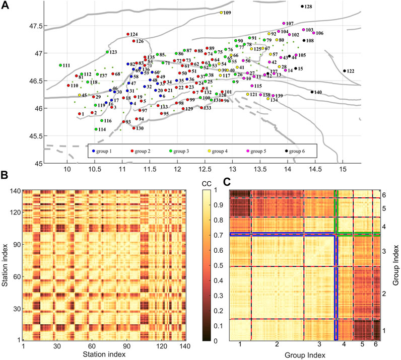
FIGURE 2. Cluster analysis for stations of similar anisotropic two-layer transverse-energy patterns. (A) Map of stations with index (as used in the correlation matrix), if at least one good measurement was recorded. The colored dots indicate the resulting six groups from the hierarchical clustering. (B) Matrix of correlation coefficients from inter-station correlation of the remaining transverse energy grid after joint splitting for two anisotropic layers. The color scales with the value of the correlation coefficient (CC). (C) Matrix of the same correlation coefficients as in (B) but sorted for groups based on the hierarchical cluster analysis with complete linkage. Six groups have been allowed (separated by red-black dashed lines), while two main groups are identified with blue (first three groups) and green (last three groups) frames.
The splitting analysis of individual events provides, in total, 3,123 pairs of splitting parameters. 792 of them are categorized as good, 1,467 as average, and 863 as null measurement. The splitting time for good and average measurements varies mainly between 1.3 ± 0.5 s and shows no major lateral variation. The dominant fast axis direction is between 50° and 65°, although there is a trend toward larger angles of 90° and up to 145°, which appear mainly with growing longitude. At first sight, the individual results can be interpreted as gentle clockwise rotation of anisotropic fast axis orientation from west to east (see Figure 3). However, the permanent stations in the east show a large variation of the individual results, which can also be seen to be less pronounced in the west. We further investigate the azimuthal distribution of the good measurements with respect to their station position in longitude (see Figure 4). The splitting measurements change laterally, mainly with longitude. The lateral and azimuthal change of the splitting parameters can be visualized in one representation, if we consider the longitude position of the station, where the measurements are recorded, as the radius in a polar plot, where the polar angle represents the back azimuth of the incoming event (see Figure 4A). While the measurements have the same lateral pattern for events coming from the opposite direction (see 45°–90° and 225°–270°, respectively), their fast axis orientation changes for events coming from different angles. This is clear evidence for the events sampling the same anisotropic origin, whereas the azimuthal variation points toward a possible anisotropic layering. Stations with a longitude greater than 13°E show the same fast axis direction for events coming from 180° to 225° and for events coming from 270° to 315°, indicating a 90° periodicity. This favors a multilayer anisotropic origin in the east. In a more classical representation of the splitting time and fast axis direction (see Figure 4B), the azimuthal variation for the stations located east of 13°E becomes evident. We estimate the two-layer characteristics of the single measurements by fitting synthetic apparent splitting parameters for a two-layer anisotropic model to our measured parameters. The synthetic splitting time and fast axis direction are calculated using the expressions introduced by Silver and Savage (1994). The apparent parameters are calculated for a two-layer model, where the splitting time of each layer is varied for 0.2 s between 0 and 4 s. The fast axis direction of each layer is varied in 10° steps between 0 and 180°. One synthetic pair of parameters for each measured pair is calculated considering the initial polarization defined by the back azimuth of the event. This allows us to define a misfit between the measured and synthetic parameters and leads to a favored model with minimum misfit. We find the best fitting model, which is defined by two equally strong anisotropic layers, an upper layer with a splitting time of 1 s and a fast axis direction of 120° and a lower layer defined by a splitting time of 1.6 s and a fast axis direction of 70°. This agrees well with the azimuthal pattern observed by Qorbani et al. (2015a) and their anisotropic model. However, while the central part of the network between 12°E and 13°E shows no significant change in the fast axis direction, a similar periodicity of weak azimuthal variation can be seen for stations west of 12°E. We investigate this further by analyzing the azimuthal variation for stations in the longitude range between 11 and 12°E. Here, we observe again a clear azimuthal variation in the splitting-parameter plots (see Figure 4C). The corresponding best fitting two-layer anisotropic model shows one dominating upper layer with a splitting time of 1.4 s and a fast axis direction of 50°. The lower layer is weaker but still considerably strong with a splitting time of 0.6 s. The fast axis direction of the deeper layer points toward 170°. This indicates a layered anisotropy for the western part of the network also, which will be further tested in a joint analysis of multiple events for two anisotropic layers in the following section. Based on the single measurements, we would expect a much smaller two-layer effect with one dominating layer (possible locally confined) in the west, compared to the east with the very pronounced variation in the anisotropic parameters.
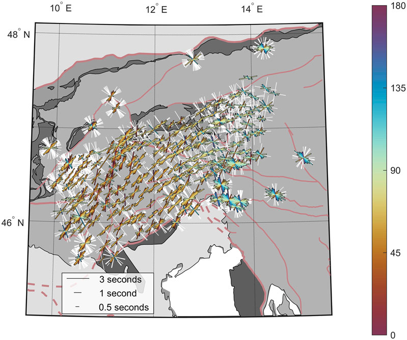
FIGURE 3. Results from single-splitting analysis. Measurements of categories good and average are presented as bars aligned with the fast axis direction and scale with strength of anisotropy. The color of the bars indicates the fast axis direction. Null measurements are shown as white crosses in the direction of the back azimuth and with 90° phase shift.
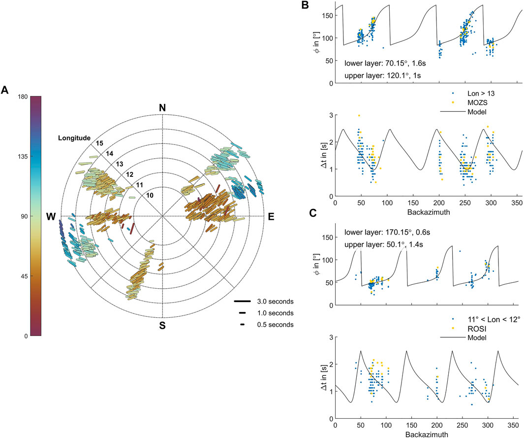
FIGURE 4. (A) Azimuthal variation of the measurements categorized as good with respect to longitude of the station (radius) and the back azimuth of the event. The color of the bars indicates the fast axis direction. (B) Synthetic apparent splitting parameters for the best fitting two-layer anisotropic model to the measurements of stations with longitude larger than 13°E (solid line). Blue circles indicate the individual splitting measurements categorized as good of all stations in this area. The yellow circles show the measurements of the exemplary station MOZS. (C) Synthetic apparent splitting parameters for the best fitting two-layer anisotropic model to the measurements of stations between the longitude of 11°E–12°E. Similar to (B) for station ROSI.
In the following section, we test the entire data set for layered anisotropy, by searching for splitting parameters of two anisotropic layers which best fit the data. We include all stations, as this analysis also allows us to test for one dominating layer with the other layer showing only minor splitting. Therefore, no previous selection on stations to be used for this analysis is necessary. A cluster analysis is performed, where we search for stations with similarities in their four-dimensional matrix of the remaining transverse energy derived from a two-layer joint-splitting analysis, as described above. We discard stations without any good measurements for this analysis to avoid a distortion caused by noise-contaminated stations. From the complete linkage using the correlation matrix of station-wise correlated four-dimensional misfit functions, we can visually identify two main groups of similar energy tensors (see Figures 2A,C), which are separated at 12.5°E–13°E. However, we allow for additional variation within these two groups by introducing six different groups in total to consider minor lateral variation in the (one- or) two-layer anisotropic pattern (compare Figure 2A).
The results from the joint splitting of the six groups all show robust splitting results (Figure 5). Three groups (1–3, see Figures 5A–C) are characterized by an upper layer with a fast axis between 55 and 70° and a lower layer with a fast axis between 1 and 37°. The splitting time of these groups (1–3) show a dominance of the upper layer with a value of 0.8–1.2 s. Only group 1 (see Figure 5A) shows a clear, pronounced second layer with a splitting time of 0.5 s and a small error for splitting time and fast axis direction in both layers. Group 2 (Figure 5B) is characterized by a considerable splitting of 0.4 s, but the error from the bootstrapping statistics of ±0.3 s shows the minor confidence in this parameter. Therefore, a one-layer solution might explain the data equally well. The splitting time for group 3 (Figure 5C) itself is very weak with only 0.2 s and is therefore also explained equally well using a one-layer model. The larger error in the fast axis direction of the lower layer is also indicative of the minor relevance of the two-layer anisotropy. For the remaining three groups (4–6, see Figures 5D–F), the lower layer shows strong splitting with a splitting time of 0.8–1 s. The fast axis direction for the lower layer shows values between 65° and 73°. While group 4 (Figure 5D) exhibits an upper layer with a splitting time of only 0.4 s, the other two groups (5 and 6, Figures 5E,F) show an equally pronounced splitting as the lower layer with 0.9 s. All three groups show a similar direction for the fast axis of the upper layer (106°–114°). Group 4 (Figure 5D) also shows a larger error for the fast axis in the weaker upper layer, which is indicative of a smaller significance of the two-layer anisotropy, similar to group 2 (Figure 5B). The two main groups (1-3 and 4–6) clearly separate into a western and an eastern subdomain at a longitude between 12.5°E and 13°E (Figure 6). This coincides with the location of the EASI profile (AlpArray Seismic Network, 2014) and also with the location between 12 and 12.5°E, where Qorbani et al. (2015a) found a transition of anisotropic effects in this region. The western part is (at least locally) characterized by a lower layer of almost N–S aligned fast axis direction (unit D in Figure 6C) and an upper layer of approximately 60° fast axis direction consistently measured for the whole western area (unit C in Figure 6C). The eastern part is characterized by a lower layer with the same direction as the previous upper layer, a fast axis direction of 60° (unit B in Figure 6C). The fast axis in the upper layer of the eastern region is aligned roughly along 110° (unit A in Figure 6C). The larger error of the fast axis direction associated with group 4 may indicate that the error is introduced by the transition from the eastern to the western area, as parts of the rays coming from the west might intersect a larger portion of the eastern regime. This lateral change is not considered in the rather simplified two-layer anisotropy, where only vertical variation is assumed. The confidence in the two-layer anisotropy for group 4 (Figure 5D) is supported by the small error in the splitting time of only 0.1 s.
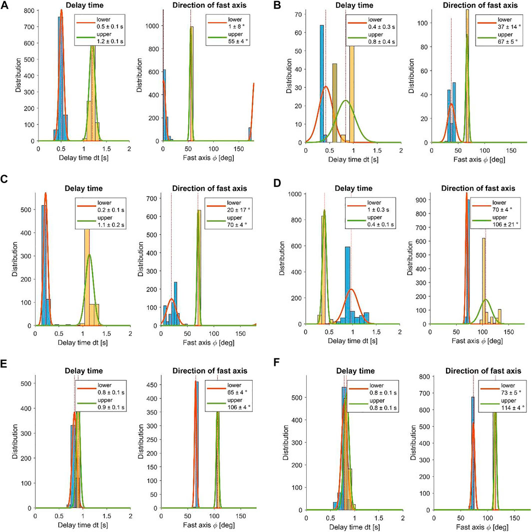
FIGURE 5. Results for the bootstrap statistics of the groups 1–6 [(A–F) in order of the groups] found in the cluster analysis. Blue bars show the histograms for the lower layer and yellow bars the histograms for the upper layer. The lines show a fit of a Gaussian curve to the distribution of each parameter given by its mean and standard deviation.
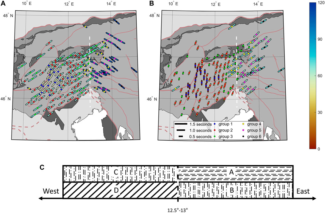
FIGURE 6. Two-layer splitting results in two separate maps indicating three different anisotropic sources. (A) Upper layer and (B) lower layer anisotropy from the joint-splitting analysis (see Figure 5). The dashed white line indicates the separation of the western and the eastern subareas at ∼13°E longitude. (C) 2D block model of main anisotropic units. A represents the upper layer in the east and B and C show the same anisotropic direction but represent the lower layer in the east (B) and the upper layer in the west (C). D represents the lower anisotropic layer in the west.
We find a lateral and a vertical variation in the anisotropic properties of the Eastern Alps, similar to Qorbani et al. (2015a). However, the statistical approach based on bootstrapping in combination with the joint-splitting analysis also allows us to identify a two-layer anisotropy for the area west of 13°E, which was previously thought to be characterized by only a single anisotropic layer (Barruol et al., 2011; Bokelmann et al., 2013; Qorbani et al., 2015a; Petrescu et al., 2020a). The dense station spacing also allows a high lateral resolution of the anisotropic pattern, which supports the abrupt change between the eastern and western parts with a distinct boundary at 12.5°E–13°E. The two-layer joint splitting allows us to separate the study area into a western and an eastern subdomain. Both domains show a layer with a fast axis of ∼60°, defining the upper layer in the west and the lower layer in the east. While the lower layer in the western subdomain shows only weak anisotropy and N–S–direction, the upper layer in the eastern subdomain is equally pronounced as the lower layer and shows a fast axis of 100°–115°.
When observing a possible vertical variation of seismic anisotropy, the crust is likely contributing at least part of this effect. Qorbani et al. (2015b) found wide similarities of single anisotropic directions to kinematic data for lower crustal material in the Tauern Window and alignment with fault structures. This is interpreted as vertical coherent deformation of the crust and the lithospheric mantle, mainly controlled by the indentation of the Adriatic microplate. Our study area is further extended to the south and covers a larger longitudinal range, which includes the main Alpine suture marked by the Tonale Fault (TF) (see also Figure 1 and Figure 7) and the Periadriatic Fault (PAF). The Giudicarie Fault (GF) differs from the mainly E–W aligned fault systems and forms a displacement of the two major faults. To investigate a possible alignment with deep-reaching surface geological features, we back-projected the individual measurements into a depth of 120 km (see Figure 7), which is the maximum base of the lithosphere for the area of the Tauern Window (Jones et al., 2010; Bianchi and Bokelmann, 2014; Qorbani et al., 2015b). While Qorbani et al. (2015b) found a very good agreement of the fast axis direction and kinematic data with the faults in the small area around the Tauern Window [in particular with the Mölltal Fault (MF)], we see such an alignment only for a limited number or only part of the faults. At the Mölltal Fault (MF), only measurements that are very close to the fault appear to align with the surface structure. They extend to the north to a region of more variable fast axis direction. A large depth extent of the fault and therefore a considerable effect is not to be expected from this very localized apparent alignment. The measurements around the Lavanttal Fault (LF) system might also be interpreted as an aligned pattern of the fast axis with the fault. However, the measurements appear to have a rotational pattern around the station location, which coincides well with the pattern of the fast axis direction for the neighboring station in the S–W and the north. This favors a deeper origin (e.g., multilayer anisotropy) as for these other stations, no alignment with surface features is visible and the rotational pattern indicates a 90° periodicity. It is remarkable that the Periadriatic Fault (PAF) and the Tonale Fault (TF), as major sutures for the European–Adriatic collision, show no significant correlation with the fast axis directions. Only the Giudicarie Fault (GF) with the northern and southern parts seems to produce a more significant imprint on the fast axis direction. The single measurements align with the fault and also show (to its west) an irregular NNE–SSW alignment along the fault, which is not visible for the measurements in the vicinity. In summary, we only see the Giudicarie Fault (GF) as a major surface feature, which seems to connect to larger depths, producing a possible anisotropic effect in the shear-wave splitting. The remaining faults seem to produce either only a very locally confined effect or produce, surprisingly, no effect at all, for example, the Periadriatic Fault (PAF) and the Tonale Fault (TF).
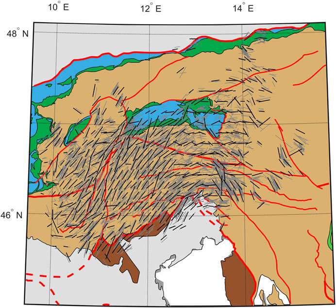
FIGURE 7. Single splitting measurements with quality good and average projected into a depth of 120 km (gray bars). For better visualization, the measurements are averaged on a regular grid, which are shown as black bars. Same tectonic map as in Figure 1.
Seismic tomography can provide insight into slab geometries and lithospheric thinning as well as asthenospheric upwelling in terms of positive and negative velocity perturbations. However, so far, studies based on body waves show only a limited agreement of velocity anomalies with flow patterns derived from shear-wave splitting (see Qorbani et al., 2015a and references therein; Lippitsch, 2003; Koulakov et al., 2009). A recent surface wave tomography by Kästle et al. (2018), Kästle et al. (2020) provides significantly improved resolution for relatively shallow structures (between 50 and 200 km). The latter shows a distinct weakening in the positive velocity perturbation of the European slab at a depth of ∼120 km at the transition to the Eastern Alps. The start of the weakening of the positive anomaly is located at a longitude of ∼13°E and therefore coincides well with the changing anisotropic pattern found in our study. This weakening can also be identified in images from body wave tomography (Zhao et al., 2016 ; Kästle et al., 2020). The weakening of the positive velocity anomaly has been interpreted as the discontinuous European slab and marks a break-off at depths of about 120–200 km. If we assume 4% anisotropy and a mantle shear velocity of 4.5 km/s, the required thickness of the anisotropic volume is about 90–100 km to satisfy the splitting times found for the upper layer in the east. The depth range between the lithospheric base and the slab fragment is found to be around 80 km and agrees with the required volume (within errors).
The dominant anisotropy (of about 60°) in the western part coincides well with the Alpine orogeny and is aligned parallel-to-subparallel to the strike of the mountain belt. This is evidence for a vertical coherent deformation with coupled anisotropy from the lithosphere to the upper asthenosphere as proposed by Silver (1996). The fast axis is not perfectly aligned with the mountain axis but shows a constant trade-off of about 10–20°. While this disagrees with an ideal coherent deformation of the crust and the mantle lithosphere, the overall regional changes of anisotropy in the Alpine area clearly rejects the simple asthenospheric flow model. In that case, the fast polarizations are expected to align more-or-less parallel to the absolute plate motion. The high variability within the plate therefore favors a shallower origin of the anisotropy. The deviation of the orogen-parallel alignment may be indicative of fossil anisotropy that is mainly preserved in the deeper crust in combination with the mantle lithosphere related to a previous stage of the European–Adriatic collision. The fast axis direction would then point to the alignment of the pre-collisional front during the subduction of the Piemont–Valais oceanic units (Handy et al., 2015).
An alternative scenario for the origin of the observed pattern in the western part of the study area is a slab-controlled flow that is mainly driven by the Adriatic intender causing a steep European subduction. The blocked mantle flow is then forced to flow around the retreating European slab, causing the alignment parallel to the orogeny (see Figure 8A, and Király et al., 2018; Petrescu et al., 2020a). Both scenarios seem equally likely for the western region, where the dominant upper layer exhibits fast axes oriented subparallel to the orogenic belt. However, our observations for the eastern subdomain show discrepancies with a slab-controlled orogen-parallel flow behind the Alpine Front; as part of the asthenospheric domain behind the slab is reoriented in the direction of the upper layer (representing the flow through the gap produced by the break-off), we would expect to observe a weakening in the slab-controlled splitting. As a consequence, the volume pushed back by the retreating slab is shortened, leading to a weaker anisotropic effect parallel to the orogeny. However, the measured direction and the strength of the anisotropy are preserved in the lower layer of the eastern subdomain and resemble the anisotropy of the upper layer in the west. Therefore, our two-layer splitting results support a lithospheric origin and the vertical coherent deformation model with orogen-parallel anisotropy or fossil anisotropy parallel to the pre-collisional subduction front (see Figure 8B). The upper layer in the east can be interpreted as an asthenospheric flow that is controlled by the break-off event, which initiated 35 Ma ago (Handy et al., 2015) when the subduction of the Tethys oceanic plate was completed. The contact of the Adriatic plate with the more rigid European continental plate favored the break-off and changed the dynamic condition in the collision. This led to a perturbation of the coherent deformation with a cancellation of the anisotropic effect in the upper lithosphere. The orogeny-parallel direction remains preserved in the detached slab fragment, which we measure as lower-layer anisotropy in the east. It may be noted that splitting observations further to the east in the Pannonian Basin and the Carpathians exhibit a similar fast axis direction to the upper layer in the eastern subdomain (Petrescu et al., 2020b and references therein). This is evidence for a larger-scale feature that is connected to the upper-layer anisotropy found in the eastern subdomain of our study area.
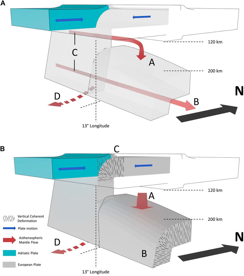
FIGURE 8. Schematic model of the lithospheric/asthenospheric interaction in the study region. A to D correspond to the anisotropic units shown in Figure 6(A–B) European plate subducts below the Adriatic plate. During the subduction process, the European plate is pushed back and produces a weak N–S directed plate motion–induced flow at the bottom of the slab (D). At around 35 Ma, a slab break-off initiated, which opened a gap for asthenospheric flow at a depth between ∼120 and ∼200 km. (A) Asthenosphere produces a toroidal flow around the retreating European slab (B and C). The opening of the break-off causes a reorientation of the minerals parallel to the orogen C into the new flow direction A of 115°N. (B) As a result of the compressive regime, anisotropy develops parallel to the orogeny (B and C) within the crust and lithosphere due to vertical coherent deformation (VCD). This anisotropy is stored in the subducting European plate. The opening of the slab break-off results in asthenospheric flow of 115°N (A). While the compressional regime in the west remains constant with the VCD causing the measured upper-layer anisotropy and plate motion–induced flow causing the lower-layer anisotropy, the change of deformation in the eastern part is perturbed by the break-off event. Here, the upper-layer anisotropy is caused by the asthenospheric flow above the detached slab, which preserves the VCD of the former collision causing the lower-layer (frozen-in) anisotropy B.
In contrast, the N–S directed anisotropy, which we resolve in the western subdomain, is quite weak and is only locally a stable feature, while the fast axis directions of all groups in the area point in a similar direction. The generally small delay times indicate less significant anisotropy or a non-horizontal fast axis, which may also be present across a wider region, but is suppressed, due to one or more dominating anisotropic layers. If we interpret the N–S directed anisotropy in the east as an asthenospheric flow below the lithosphere, such large-scale distribution would be necessary. The asthenospheric flow would then represent the return flow of mantle material following the dip of the subducting plate and submerge below the retreating European slab that is pushed by the Adriatic intender (see Figure 8 and compare with Funiciello et al., 2006 for laboratory experiments). The close vicinity of the group with clear two-layer results in the west to the Giudicarie Fault might favor this geologic feature as the origin of an apparent two-layer effect. As the back-projected single measurements also show an alignment with the fault (see Figure 7), this provides additional evidence for a deep-reaching fault, which affects the splitting. While the order of the layers is a counterargument, as the N–S layer (parallel to the strike of the fault) is found to be the lower layer in contrast to the shallow surface feature, the conditions for the two-layer analysis are not ideal. The number of measurements and the azimuthal coverage are limited. It seems logical that the laterally confined feature of the fault leads to an effect on events of only a limited azimuthal range. That, in combination with the limited azimuthal event coverage, can lead to an apparent two-layer model. Still, the strong effect on the splitting measurements requires a deep-reaching fault likely extending into the mantle lithosphere. This is not supported by Moho contours of the suture, where a displacement, as seen at the surface, is not visible (Spada et al., 2013; Handy et al., 2015). Whether the measured two-layer effect in the western subdomain originates in the mantle or is influenced by the crust could be resolved with a longer measurement period of a similarly dense network. This would allow the application of techniques based on receiver functions or ambient noise, which may be able to resolve shallower features in more detail.
This study addresses the open questions regarding a possible slab break-off accompanied by a subduction polarity flip in the transition of the Central to the Eastern Alps. We approach this question based on tectonic implications given by shear-wave splitting measurements at the dense SWATH-D complementary network and stations of the AlpArray backbone in the same area. As previous studies imply a two-layer anisotropy in the Eastern Alps (Qorbani et al., 2015a), we investigate this further and search for a possible two-layer anisotropic model. A depth-dependent anisotropic structure is also supported by the observed azimuthal variation of the single splitting measurements. The temporary character of the SWATH-D experiment and the associated limited amount of data do not allow for a conventional single-station two-layer analysis in this area. Therefore, we combine measurements of multiple stations based on a cluster analysis to resolve the splitting parameters of two layers. While allowing for further variation in up to six groups, the cluster analysis yields two main groups of similar splitting effects separated approximately at a longitude of 13°E. The western part is characterized by a lower layer of N–S direction and an upper layer with a fast direction of roughly 60°. The eastern part shows a lower layer with a fast direction of 60° and an upper layer with a fast direction of 110°, which is in agreement with previous observations (Qorbani et al., 2015a).
As the upper layer of the western part shows the same direction as the lower layer in the east, a common origin for the anisotropy seems likely. We interpret this as lithospheric anisotropy frozen in the European subducting slab with vertical coupling into the asthenosphere. Weak N–S aligned anisotropy in the west indicates either a return flow at the bottom of the retreating European slab pushed by the Adriatic plate or, alternatively, a deep-reaching Giudicarie Fault, which may produce an apparent two-layer effect. The abrupt change of the two-layer anisotropic pattern with an equally pronounced splitting of the upper layer in the east is evidence for a break-off event initiated 35 Ma ago (Handy et al., 2015). While the slab fragment is sinking into the mantle (a connection to the European slab is likely to remain), the gap provides an opening for asthenospheric flow from the Alpine Front to the Pannonian Basin.
While this interpretation provides evidence for the subduction of the European plate below the Adriatic intender with a break-off event in the eastern part of the Alps, the splitting measurements cannot constrain a possible subsequent subduction of the Adriatic plate below Europe, filling the gap (Lippitsch, 2003; Handy et al., 2015; Kästle et al., 2020). Therefore, further investigation is required to resolve the subduction polarity in the Eastern Alps.
Publicly available datasets were analyzed in this study. These data can be found here: ZS, GEOFON Data Archive (doi: 10.14470/MF7562601148); BW, Department of Earth and Environmental Sciences, Geophysical Observatory, University of Munchen (doi: 10.7914/SN/BW); CH, Swiss Seismological Service (SED) at ETH Zurich (doi: 10.12686/sed/networks/ch); IV, SI, INGV Seismological Data Centre (doi: 10.13127/SD/X0FXnH7QfY); NI, OGS (Istituto Nazionale di Oceanografia e di Geofisica Sperimentale) and University of Trieste (doi: 10.7914/SN/NI); OE: ZAMG-Zentralanstalt für Meterologie und Geodynamik (doi: 10.7914/SN/OE); OX, OGS (Istituto Nazionale di Oceanografia e di Geofisica Sperimentale) (doi: 10.7914/SN/OX); SL, Slovenian Environment Agency (doi: 10.7914/SN/SL).
FL developed and performed the data analysis and wrote the first draft of the manuscript. FL and GR jointly discussed the results and their interpretation and revised the manuscript.
This study was supported by the Deutsche Forschungsgemeinschaft (DFG) within the priority program “Mountain Building Processes in Four Dimensions” (SPP 4D-MB).
The authors declare that the research was conducted in the absence of any commercial or financial relationships that could be construed as a potential conflict of interest.
The handling editor GH and the reviewers SS and GB declared a shared research group, the AlpArray Working Group, with one of the authors, GR, at the time of review.
All claims expressed in this article are solely those of the authors and do not necessarily represent those of their affiliated organizations, or those of the publisher, the editors, and the reviewers. Any product that may be evaluated in this article, or claim that may be made by its manufacturer, is not guaranteed or endorsed by the publisher.
We would like to thank two reviewers for their constructive and very helpful comments. We acknowledge the operation of the SWATH-D complementary seismic network with the support of the Geophysical Instrument Pool Potsdam (GIPP), see Heit al. (2017), and the permanent seismic networks used in this study: BW, Department of Earth and Environmental Sciences, Geophysical Observatory, University of München; CH, Swiss Seismological Service (SED) at ETH Zurich; IV, SI, INGV Seismological Data Centre; NI, OGS (Istituto Nazionale di Oceanografia e di Geofisica Sperimentale) and University of Trieste; OE: ZAMG-Zentralanstalt für Meterologie und Geodynamik; OX, OGS (Istituto Nazionale di Oceanografia e di Geofisica Sperimentale); SL, Slovenian Environment Agency. We acknowledge the scientific exchange and cooperation within the AlpArray Working Group (http://www.alparray.ethz.ch) and would like to thank the AlpArray Seismic Network Team: György HETÉNYI, Rafael ABREU, Ivo ALLEGRETTI, Maria-Theresia APOLONER, Coralie AUBERT, Simon BESANÇON, Maxime BÈS DE BERC, Götz BOKELMANN, Didier BRUNEL, Marco CAPELLO, Martina ČARMAN, Adriano CAVALIERE, Jérôme CHÈZE, Claudio CHIARABBA, John CLINTON, Glenn COUGOULAT, Wayne C. CRAWFORD, Luigia CRISTIANO, Tibor CZIFRA, Ezio D'ALEMA, Stefania DANESI, Romuald DANIEL, Anke DANNOWSKI, Iva DASOVIĆ, Anne DESCHAMPS, Jean-Xavier DESSA, Cécile DOUBRE, Sven EGDORF, ETHZ-SED Electronics Lab, Tomislav FIKET, Kasper FISCHER, Wolfgang FRIEDERICH, Florian FUCHS, Sigward FUNKE, Domenico GIARDINI, Aladino GOVONI, Zoltán GRÁCZER, Gidera GRÖSCHL, Stefan HEIMERS, Ben HEIT, Davorka HERAK, Marijan HERAK, Johann HUBER, Dejan JARIĆ, Petr JEDLIČKA, Yan JIA, Hélène JUND, Edi KISSLING, Stefan KLINGEN, Bernhard KLOTZ, Petr KOLÍNSKÝ, Heidrun KOPP, Michael KORN, Josef KOTEK, Lothar KÜHNE, Krešo KUK, Dietrich LANGE, Jürgen LOOS, Sara LOVATI, Deny MALENGROS, Lucia MARGHERITI, Christophe MARON, Xavier MARTIN, Marco MASSA, Francesco MAZZARINI, Thomas MEIER, Laurent MÉTRAL, Irene MOLINARI, Milena MORETTI, Anna NARDI, Jurij PAHOR, Anne PAUL, Catherine PÉQUEGNAT, Daniel PETERSEN, Damiano PESARESI, Davide PICCININI, Claudia PIROMALLO, Thomas PLENEFISCH, Jaroslava PLOMEROVÁ, Silvia PONDRELLI, Snježan PREVOLNIK, Roman RACINE, Marc RÉGNIER, Miriam REISS, Joachim RITTER, Georg RÜMPKER, Simone SALIMBENI, Marco SANTULIN, Werner SCHERER, Sven SCHIPPKUS, Detlef SCHULTE-KORTNACK, Vesna ŠIPKA, Stefano SOLARINO, Daniele SPALLAROSSA, Kathrin SPIEKER, Josip STIPČEVIĆ, Angelo STROLLO, Bálint SÜLE, Gyöngyvér SZANYI, Eszter SZŰCS, Christine THOMAS, Martin THORWART, Frederik TILMANN, Stefan UEDING, Massimiliano VALLOCCHIA, Luděk VECSEY, René VOIGT, Joachim WASSERMANN, Zoltán WÉBER, Christian WEIDLE, Viktor WESZTERGOM, Gauthier WEYLAND, Stefan WIEMER, Felix WOLF, David WOLYNIEC, Thomas ZIEKE, Mladen ŽIVČIĆ and Helena ŽLEBČÍKOVÁ. We would also like to thank to the SWATH-D Working Group: Ben HEIT, Michael WEBER, Christian HABERLAND, Frederik TILMANN (Helmholtz-Zentrum Potsdam Deutsches GeoForschungsZentrum [GFZ]) and the SWATH-D Field Team: Luigia CHRISTIANO, Peter PILZ, Camilla CATTANIA, Francesco MACCAFERRI, Angelo STROLLO, Susanne HEMMLEB, Stefan MROCZEK, Thomas ZIEKE, Günter ASCH, Peter WIGGER, James MECHIE, Karl OTTO, Patricia RITTER, Djamil AL-HALBOUNI, Alexandra MAUERBERGER, Ariane SIEBERT, Leonard GRABOW, Xiaohui YUAN, Christoph SENS-SCHONFELDER, Jennifer DREILING, Rob GREEN, Lorenzo MANTILONI, Jennifer JENKINS, Alexander JORDAN, Azam Jozi NAJAFABADI, Susanne KALLENBACH (Helmholtz-Zentrum Potsdam Deutsches GeoForschungsZentrum [GFZ]), Ludwig KUHN, Florian DORGERLOH, Stefan MAUERBERGER, Jan SEIDEMANN (Universität Potsdam), Rens HOFMAN (Freie Universität Berlin), Nikolaus HORN, Stefan WEGINGER, Anton VOGELMANN (Austria: Zentralanstalt für Meteorologie und Geodynamik [ZAMG]), Simone KASEMANN (Universität Bremen), Claudio CARRARO, Corrado MORELLI (Südtirol/Bozen: Amt für Geologie und Baustoffprüfung), Günther WALCHER, Martin PERNTER, Markus RAUCH (Civil Protection Bozen), Giorgio DURI, Michele BERTONI, Paolo FABRIS (Istituto Nazionale di Oceanografia e di Geofisica Sperimentale [OGS] [CRS Udine]), Andrea FRANCESCHINI, Mauro ZAMBOTTO, Luca FRONER, Marco GARBIN (also OGS) (Ufficio Studi Sismici e Geotecnici-Trento).
The Supplementary Material for this article can be found online at: https://www.frontiersin.org/articles/10.3389/feart.2021.679887/full#supplementary-material
AlpArray Seismic Network (2015). AlpArray Seismic Network (AASN) Temporary component. AlpArray Working Group. Other/Seismic Network. doi:10.12686/alparray/z3_2015
AlpArray Seismic Network (2014). Eastern Alpine Seismic Investigation (EASI) - AlpArray Complementary Experiment. AlpArray Working Group. doi:10.12686/alparray/xt_2014
Backus, G. E. (1962). Long-wave elastic anisotropy produced by horizontal layering. J. Geophys. Res. 67, 4427–4440. doi:10.1029/jz067i011p04427
Barruol, G., Bonnin, M., Pedersen, H., Bokelmann, G. H. R., and Tiberi, C. (2011). Belt-parallel mantle flow beneath a halted continental collision: The Western Alps. Earth Planet. Sci. Lett. 302, 429–438. doi:10.1016/j.epsl.2010.12.040
Bianchi, I., and Bokelmann, G. (2014). Seismic signature of the Alpine indentation, evidence from the Eastern Alps. J. geodynamics 82, 69–77. doi:10.1016/j.jog.2014.07.005
Bigi, G., Cosentino, D., Parotto, M., Sartori, R., and Scandone, P. (1992). Structural model of Italy, 1:500.000. CNR Progetto Finalizzato Geodinamica 114 (3).
Bokelmann, G., Qorbani, E., and Bianchi, I. (2013). Seismic anisotropy and large-scale deformation of the Eastern Alps. Earth Planet. Sci. Lett. 383, 1–6. doi:10.1016/j.epsl.2013.09.019
Bousquet, R., Schmid, S. M., Zeilinger, G., Oberhänsli, R., Rosenberg, C., Molli, G., et al. (2012). “Tectonic framework of the Alps,” in Lithosphere Structure and Tectonics of the Alps (Paris: CCGM/CGMW).
Christensen, N. I. (1966). Shear wave velocities in metamorphic rocks at pressures to 10 kilobars. J. Geophys. Res. 71, 3549–3556. doi:10.1029/jz071i014p03549
Crampin, S. (1987). The basis for earthquake prediction. Geophys. J. Int. 91, 331–347. doi:10.1111/j.1365-246X.1987.tb05230.x
Dewey, J. F., Helman, M. L., Knott, S. D., Turco, E., and Hutton, D. H. W. (1989). Kinematics of the western Mediterranean. Geol. Soc. Lond. Spec. Publications 45 (1), 265–283. doi:10.1144/gsl.sp.1989.045.01.15
Dewey, J. F., Pitman, W. C., Ryan, W., and Bonnin, J. (1973). Plate Tectonics and the evolution of the Alpine system. Geol. Soc. America Bull. 84 (10), 3137–3180. doi:10.1130/0016-7606(1973)84<3137:ptateo>2.0.co;2
Efron, B. (1992). Bootstrap Methods: Another Look at the Jackknife. Ann. Stat. 7 (1), 569–593. doi:10.1007/978-1-4612-4380-9_41
Everitt, B. S., Landau, S., Leese, M., and Stahl, D. (2011). Cluster Analysis Chichester: Wiley. doi:10.1002/9780470977811
Froitzheim, N., Schmid, S. M., and Frey, M. (1996). Mesozoic paleogeography and the Timing of eclogite-facies metamorphism in the Alps: A working hypothesis. Eclogae Geologicae Helv. 89 (1), 81.
Funiciello, F., Moroni, M., Piromallo, C., Faccenna, C., Cenedese, A., and Bui, H. A. (2006). Mapping mantle flow during retreating subduction: Laboratory models analyzed by feature Tracking. J. Geophys. Res. 111 (B3), a–n. doi:10.1029/2005jb003792
Handy, M. R., Giese, J., Schmid, S. M., Pleuger, J., Spakman, W., Onuzi, K., et al. (2019). Coupled Crust‐Mantle Response to Slab Tearing, Bending, and Rollback Along the Dinaride‐Hellenide Orogen. Tectonics 38, 2803–2828. doi:10.1029/2019tc005524
Handy, M. R., M. Schmid, S., Bousquet, R., Kissling, E., and Bernoulli, D. (2010). Reconciling plate-Tectonic reconstructions of Alpine Tethys with the geological-geophysical record of spreading and subduction in the Alps. Earth-Science Rev. 102, 121–158. doi:10.1016/j.earscirev.2010.06.002
Handy, M. R., Ustaszewski, K., and Kissling, E. (2015). Reconstructing the Alps-Carpathians-Dinarides as a key to understanding switches in subduction polarity, slab gaps and surface motion. Int. J. Earth Sci. (Geol Rundsch) 104, 1–26. doi:10.1007/s00531-014-1060-3
Harangi, S., Downes, H., and Seghedi, I. (2006). Tertiary-Quaternary subduction processes and related magmatism in the Alpine-Mediterranean region. Geol. Soc. Lond. Mem. 32, 167–190. doi:10.1144/gsl.mem.2006.032.01.10
Heit, B., Weber, M., Tilmann, F., Haberland, C., Jia, Y., and Pesaresi, D. (2017). The Swath-D Seismic Network in Italy and Austria. GFZ Data Services. Other/Seismic Network. doi:10.14470/MF7562601148
Hetényi, G., Molinari, I., Molinari, I., Clinton, J., Bokelmann, G., Bondár, I., et al. (2018a). The AlpArray seismic network: a large-scale European experiment to image the Alpine orogen. Surv. Geophys. 39 (5), 1009–1033. doi:10.1007/s10712-018-9472-4
Hetényi, G., Plomerová, J., Bianchi, I., Kampfová Exnerová, H., Bokelmann, G., Handy, M. R., et al. (2018b). From mountain summits to roots: Crustal structure of the Eastern Alps and Bohemian Massif along longitude 13.3°E. Tectonophysics 744, 239–255. doi:10.1016/j.tecto.2018.07.001
Homuth, B., Löbl, U., Batte, A. G., Link, K., Kasereka, C. M., and Rümpker, G. (2016). Seismic anisotropy of the lithosphere/asthenosphere system beneath the Rwenzori region of the Albertine Rift. Int. J. Earth Sci. (Geol Rundsch) 105, 1681–1692. doi:10.1007/s00531-014-1047-0
Jones, A. G., Plomerova, J., Korja, T., Sodoudi, F., and Spakman, W. (2010). Europe from the bottom up: A statistical examination of the central and northern European lithosphere-asthenosphere boundary from comparing seismological and electromagnetic observations. Lithos 120, 14–29. doi:10.1016/j.lithos.2010.07.013
Karato, S.-i., Jung, H., Katayama, I., and Skemer, P. (2008). Geodynamic Significance of Seismic Anisotropy of the Upper Mantle: New Insights from Laboratory Studies. Annu. Rev. Earth Planet. Sci. 36, 59–95. doi:10.1146/annurev.earth.36.031207.124120
Kästle, E. D., El-Sharkawy, A., Boschi, L., Meier, T., Rosenberg, C., Bellahsen, N., et al. (2018). Surface Wave Tomography of the Alps Using Ambient-Noise and Earthquake Phase Velocity Measurements. J. Geophys. Res. Solid Earth 123 (2), 1770–1792. doi:10.1002/2017jb014698
Kästle, E. D., Rosenberg, C., Boschi, L., Bellahsen, N., Meier, T., and El-Sharkawy, A. (2020). Slab break-offs in the Alpine subduction zone. Int. J. Earth Sci. (Geol Rundsch) 109, 587–603. doi:10.1007/s00531-020-01821-z
Király, Á., Faccenna, C., and Funiciello, F. (2018). Subduction Zones Interaction Around the Adria Microplate and the Origin of the Apenninic Arc. Tectonics 37, 3941–3953. doi:10.1029/2018tc005211
Kissling, E., Schmid, S. M., Lippitsch, R., Ansorge, J., and Fügenschuh, B. (2006). Lithosphere structure and Tectonic evolution of the Alpine arc: new evidence from high-resolution Teleseismic Tomography. Geol. Soc. Lond. Mem. 32, 129–145. doi:10.1144/gsl.mem.2006.032.01.08
Koulakov, I., Kaban, M. K., Tesauro, M., and Cloetingh, S. (2009). P- andS-velocity anomalies in the upper mantle beneath Europe from Tomographic inversion of ISC data. Geophys. J. Int. 179 (1), 345–366. doi:10.1111/j.1365-246x.2009.04279.x
Lippitsch, R. (2003). Upper mantle structure beneath the Alpine orogen from high-resolution Teleseismic Tomography. J. Geophys. Res. 108. doi:10.1029/2002jb002016
Long, M. D., and Becker, T. W. (2010). Mantle dynamics and seismic anisotropy. Earth Planet. Sci. Lett. 297, 341–354. doi:10.1016/j.epsl.2010.06.036
Lüschen, E., Lammerer, B., Gebrande, H., Millahn, K., and Nicolich, R. (2004). Orogenic structure of the Eastern Alps, Europe, from TRANSALP deep seismic reflection profiling. Tectonophysics 388, 85–102. doi:10.1016/j.tecto.2004.07.024
Menke, W., and Levin, V. (2003). The cross-convolution method for interpretingSKSsplitting observations, with application to one and Two-layer anisotropic earth models. Geophys. J. Int. 154 (2), 379–392. doi:10.1046/j.1365-246x.2003.01937.x
Molli, G., and Malavieille, J. (2011). Orogenic processes and the Corsica/Apennines geodynamic evolution: insights from Taiwan. Int. J. Earth Sci. (Geol Rundsch) 100, 1207–1224. doi:10.1007/s00531-010-0598-y
Nur, A. (1971). Effects of Stress on Velocity Anisotropy in Rocks With Cracks. J. Geophy. Res. 76 (8), 2022–2034. doi:10.1029/JB076I008P02022
Nur, A., and Simmons, G. (1969). Stress-induced velocity anisotropy in rock: An experimental study. J. Geophys. Res. 74 (27), 6667–6674. doi:10.1029/jb074i027p06667
Petrescu, L., Pondrelli, S., Salimbeni, S., Faccenda, M., and Group, A. W. (2020a). Mantle flow below the central and greater Alpine region: insights from SKS anisotropy analysis at AlpArray and permanent stations. Solid Earth 11 (4), 1275–1290. doi:10.5194/se-11-1275-2020
Petrescu, L., Stuart, G., Houseman, G., and Bastow, I. (2020b). Upper mantle deformation signatures of craton-orogen interaction in the Carpathian-Pannonian region from SKS anisotropy analysis. Geophys. J. Int. 220 (3), 2105–2118. doi:10.1093/gji/ggz573
Qorbani, E., Bianchi, I., and Bokelmann, G. (2015a). Slab detachment under the Eastern Alps seen by seismic anisotropy. Earth Planet. Sci. Lett. 409 (1), 96–108. doi:10.1016/j.epsl.2014.10.049
Qorbani, E., Kurz, W., Bianchi, I., and Bökelmann, G. (2015b). Correlated crustal and mantle deformation in the Tauern Window, Eastern Alps. Ajes 108, 159–171. doi:10.17738/ajes.2015.0010
Reiss, M. C., and Rümpker, G. (2017). SplitRacer: MATLAB Code and GUI for Semiautomated Analysis and Interpretation of Teleseismic Shear‐Wave Splitting. Seismological Res. Lett. 88 (2A), 392–409. doi:10.1785/0220160191
Reiss, M. C., Rümpker, G., Tilmann, F., Yuan, X., Giese, J., and Rindraharisaona, E. J. (2016). Seismic anisotropy of the lithosphere and asthenosphere beneath southern Madagascar from Teleseismic shear wave splitting analysis and waveform modeling. J. Geophys. Res. Solid Earth 121, 6627–6643. doi:10.1002/2016jb013020
Reiss, M. C., Rümpker, G., and Wölbern, I. (2018). Large-scale Trench-normal mantle flow beneath central South America. Earth Planet. Sci. Lett. 482, 115–125. doi:10.1016/j.epsl.2017.11.002
Rümpker, G., and Silver, P. G. (1998). Apparent shear-wave splitting parameters in the presence of vertically varying anisotropy. Geophys. J. Int. 135 (3), 790–800. doi:10.1046/j.1365-246x.1998.00660.x
Savage, M. K. (1999). Seismic anisotropy and mantle deformation: What have we learned from shear wave splitting? Rev. Geophys. 37, 65–106. doi:10.1029/98RG02075
Schmid, S. M., Bernoulli, D., Fügenschuh, B., Matenco, L., Schefer, S., Schuster, R., et al. (2008). The Alpine-Carpathian-Dinaridic orogenic system: correlation and evolution of Tectonic units. Swiss J. Geosci. 101, 139–183. doi:10.1007/s00015-008-1247-3
Schmid, S. M., Fügenschuh, B., Kissling, E., and Schuster, R. (2004). Tectonic map and overall architecture of the Alpine orogen. Eclogae geol. Helv. 97, 93–117. doi:10.1007/s00015-004-1113-x
Schmid, S. M., Scharf, A., Handy, M. R., and Rosenberg, C. L. (2013). The Tauern Window (Eastern Alps, Austria): a new Tectonic map, with cross-sections and a Tectonometamorphic synthesis. Swiss J. Geosci. 106, 1–32. doi:10.1007/s00015-013-0123-y
Silver, P. G., and Chan, W. W. (1991). Shear wave splitting and subcontinental mantle deformation. J. Geophys. Res. 96 (B10), 16429–16454. doi:10.1029/91JB00899
Silver, P. G., and Savage, M. K. (1994). The interpretation of shear-wave splitting parameters in the presence of Two anisotropic layers. Geophys. J. Int. 119 (3), 949–963. doi:10.1111/j.1365-246x.1994.tb04027.x
Silver, P. G. (1996). Seismic anisotropy beneath the continents: Probing the depths of geology. Annu. Rev. Earth Planet. Sci. 24 (1), 385–432. doi:10.1146/annurev.earth.24.1.385
Spada, M., Bianchi, I., Kissling, E., Agostinetti, N. P., and Wiemer, S. (2013). Combining controlled-source seismology and receiver function information to derive 3-D Moho Topography for Italy. Geophys. J. Int. 194, 1050–1068. doi:10.1093/gji/ggt148
Ustaszewski, K., Schmid, S. M., Fügenschuh, B., Tischler, M., Kissling, E., and Spakman, W. (2008). A map-view restoration of the Alpine-Carpathian-Dinaridic system for the Early Miocene. Swiss J. Geosci. 101, 273–294. doi:10.1007/s00015-008-1288-7
Vignaroli, G., Faccenna, C., Jolivet, L., Piromallo, C., and Rossetti, F. (2008). Subduction polarity reversal at the junction between the Western Alps and the Northern Apennines, Italy. Tectonophysics 450, 34–50. doi:10.1016/j.tecto.2007.12.012
von Blanckenburg, F., and Davies, J. H. (1995). Slab breakoff: A model for syncollisional magmatism and Tectonics in the Alps. Tectonics 14, 120–131. doi:10.1029/94tc02051
Yousef, B. M., and Angus, D. A. (2016). When do fractured media become seismically anisotropic? Some implications on quantifying fracture properties. Earth Planet. Sci. Lett. 444, 150–159. doi:10.1016/j.epsl.2016.03.040
Yuan, H., Dueker, K., and Schutt, D. L. (2008). Testing five of the simplest upper mantle anisotropic velocity parameterizations using Teleseismic S and SKS data from the Billings, Montana PASSCAL array. J. Geophys. Res. 113, B03304. doi:10.1029/2007jb005092
Keywords: shear-wave splitting, cluster analysis, anisotropy, mantle flow, Alpine orogeny, Eastern Alps, lithosphere, asthenosphere
Citation: Link F and Rümpker G (2021) Resolving Seismic Anisotropy of the Lithosphere–Asthenosphere in the Central/Eastern Alps Beneath the SWATH-D Network. Front. Earth Sci. 9:679887. doi: 10.3389/feart.2021.679887
Received: 12 March 2021; Accepted: 16 July 2021;
Published: 03 September 2021.
Edited by:
György Hetényi, University of Lausanne, SwitzerlandReviewed by:
Götz Bokelmann, University of Vienna, AustriaCopyright © 2021 Link and Rümpker. This is an open-access article distributed under the terms of the Creative Commons Attribution License (CC BY). The use, distribution or reproduction in other forums is permitted, provided the original author(s) and the copyright owner(s) are credited and that the original publication in this journal is cited, in accordance with accepted academic practice. No use, distribution or reproduction is permitted which does not comply with these terms.
*Correspondence: Frederik Link, bGlua0BnZW9waHlzaWsudW5pLWZyYW5rZnVydC5kZQ==
Disclaimer: All claims expressed in this article are solely those of the authors and do not necessarily represent those of their affiliated organizations, or those of the publisher, the editors and the reviewers. Any product that may be evaluated in this article or claim that may be made by its manufacturer is not guaranteed or endorsed by the publisher.
Research integrity at Frontiers
Learn more about the work of our research integrity team to safeguard the quality of each article we publish.