Evaluation of Remote Mapping Techniques for Earthquake-Triggered Landslide Inventories in an Urban Subarctic Environment: A Case Study of the 2018 Anchorage, Alaska Earthquake

Earthquake-induced landslide inventories can be generated using field observations but doing so can be challenging if the affected landscape is large or inaccessible after an earthquake. Remote sensing data can be used to help overcome these limitations. The effectiveness of remotely sensed data to produce landslide inventories, however, is dependent on a variety of factors, such as the extent of coverage, timing, and data quality, as well as environmental factors such as atmospheric interference (e.g., clouds, water vapor) or snow and vegetation cover. With these challenges in mind, we use a combination of field observations and remote sensing data from multispectral, light detection and ranging (lidar), and synthetic aperture radar (SAR) sensors to produce a ground failure inventory for the urban areas affected by the 2018 magnitude (M_w) 7.1 Anchorage, Alaska earthquake. The earthquake occurred during late November at high latitude (∼61°N), and the lack of sunlight, persistent cloud cover, and snow cover that occurred after the earthquake made remote mapping challenging for this event. Despite these challenges, 43 landslides were manually mapped and classified using a combination of the datasets mentioned previously. Using this manually compiled inventory, we investigate the individual performance and reliability of three remote sensing techniques in this environment not typically hospitable to remotely sensed mapping. We found that differencing pre- and post-event normalized difference vegetation index maps and lidar worked best for identifying soil slumps and rapid soil flows, but not as well for small soil slides, soil block slides and rock falls. The SAR-based methods did not work well for identifying any landslide types because of high noise levels likely related to snow. Some landslides, especially those that resulted in minor surface displacement, were identifiable only from the field observations. This work highlights the importance of the rapid collection of field observations and provides guidance for future mappers on which techniques, or combination of techniques, will be most effective at remotely mapping landslides in a subarctic and urban environment.

Introduction

The November 30, 2018 magnitude (M_w) 7.1 Anchorage, Alaska earthquake, triggered substantial ground failure throughout Anchorage and surrounding areas (Grant et al., 2020b; Jibson et al., 2020). The earthquake was an intraslab event with a focal depth of about 47 km and an epicenter about 16 km north of the city of Anchorage. Most of the landslides triggered by the earthquake were small (<15,000 m²), and shallow, attributed to the relatively short duration of ground motion (1 min) and deep source, which resulted in widespread shaking but without high peak ground accelerations (Grant et al., 2020b; Jibson et al., 2020). Peak ground accelerations reached ∼30% g. Despite the relatively subdued ground failure, geotechnical damage to buildings and structures was widespread (Franke et al., 2019). The last major earthquake to significantly damage Anchorage was the 1964 M 9.2 Great Alaska earthquake, a subduction zone earthquake that shook the city at similar levels to the 2018 earthquake but for 4–7 min and caused extensive landslide damage, including large translational landslides in developed areas of the city (Hansen, 1965).

The 2018 earthquake is an important ground failure event to document thoroughly not only because of the region’s history of earthquake-triggered ground failure, but also as a key dataset needed to improve hazard characterization in other geologically and climatically similar regions in the world. Documenting events with subdued ground failure is important because these events are underrepresented in existing inventories. Field-based observations, photos, and ground failure features recorded by U.S. Geological Survey (USGS) scientists during the 10 days immediately following the earthquake are summarized in Grant et al. (2020a) and Jibson et al. (2020). However, around the time of the earthquake, Anchorage was experiencing approximately 6 h of daylight between 09:45 and 15:50, which limited field observations. A cumulative total of 0.109 m of snowfall occurred in Anchorage the 10 days following the earthquake (NOAA/NWS Interactive Snow Information https://www.nohrsc.noaa.gov/interactive), which also obscured overflight observations, particularly at higher elevations (Grant et al., 2020b; Jibson et al., 2020). Partial or complete snow coverage persisted until late March (NOAA/NWS Interactive Snow Information). Grant et al. (2020b) and Jibson et al. (2020) note that their observations are generally incomplete due to these adverse conditions experienced while collecting data.

Our long-term goal is to produce a complete and high-quality landslide inventory associated with this event. The data collected in the field, however, were not sufficient to build such an inventory. The adverse conditions experienced indicate that an inventory built solely on these data would be incomplete because some landslide features may have been obscured by snowfall or simply not documented (i.e., those landslides in areas not easily accessible). Thus, we built an inventory by using both the field observation data and remotely sensed data as they supplement one another. To assemble our inventory, we first identified the location of landslide features by comparing the field observation data (photos) to high-resolution satellite imagery (WorldView-2, WorldView-3, GeoEye-1). Once the location of the landslide was determined, we used a variety of remote sensing methods to locate the head scarp of the landslide feature and to also delineate the landslide where possible. In creating our inventory, we found that the effectiveness of remote sensing data to identify and delineate landslides in this environment varied. In our study area, some field-verified landslides could be identified and delineated using multiple methods while others could not be identified at all. Our inventory allowed us to determine the capabilities and limitations of remotely sensed data to map landslides in an environment such as Anchorage. This knowledge can be used to guide remote mapping beyond the field area and help us achieve our goal of eventually creating a complete landslide inventory.

We use the landslide inventory to retroactively evaluate the effectiveness of the three remote sensing methods used: 1) light detection and ranging (lidar) elevation differencing, 2) normalized difference vegetation index (NDVI) differencing, and 3) synthetic aperture radar (SAR) amplitude change detection (ACD). We compare these methods against the inventory data in a subarea of Anchorage for which data for all three methods are available. For clarity, we refer to this subarea as the study area. We describe the effectiveness of each method to identify certain landslide types and why some methods may have outperformed others. Additionally, we identify environmental and data-type specific challenges. While such an analysis will help in our efforts to build a complete inventory beyond the study area, this work can aid others in remote mapping as well.

Background

The location, size, and spatial distribution of landslides can help define regional landslide trends, reveal geologic and structural patterns of a given environment, and inform landslide hazard and susceptibility models (e.g., Keefer, 1984; Mirus et al., 2020). Landslide inventories have long provided the foundation for a wide variety of landslide research, such as updating and improving landslide susceptibility models (Stanley and Kirschbaum, 2017; Nowicki Jessee et al., 2018), optimizing empirical and deterministic criteria for landslide early warning systems (Baum et al., 2010; Mirus et al., 2018), or understanding the role of hillslope erosion in landscape evolution (Larsen and Montgomery, 2012). Thus, compiling landslide inventories after triggering events (e.g., earthquake, rainfall) is highly beneficial for landslide hazard assessment and risk reduction efforts.

Recent studies have emphasized the importance of landslide inventory quality across a variety of triggering scenarios, landscapes, and climates for landslide studies and model development (Tanyaş et al., 2017; Mirus et al., 2020; Tanyaş and Lombardo, 2020). The accuracy and completeness of landslide inventories vary due to data quality, accessibility, and availability, as well as event-specific field conditions and accessibility. Limitations in data resolution or field observations also result in infrequent documentation of the smallest landslides triggered by a seismic or rainfall event (Guzzetti et al., 2012). Additionally, the end goals and purpose for creating landslide inventories differ between authors and across organizations, resulting in varying levels of detail and data inclusion (e.g., Mirus et al., 2020).

Many advancements in landslide mapping and inventory quality can be linked to the increasing availability and attainability of remotely sensed imagery that aid in large scale mapping (Guzzetti et al., 2012), complementing traditional field observations. Manual image interpretation or automatic detection methods can be used with a variety of aerial and satellite data products, such as optical (visual) images, multispectral images, laser scanning, and radar sensors to develop inventories (Booth et al., 2009; Martha et al., 2011; Harp et al., 2016; Mondini et al., 2019). The quality of inventories developed using each approach varies, however, and is dependent on a few variables. For example, manual interpretation of imagery can be limited by the resolution of data and experience of the mapper and can be time intensive depending on the level of detail desired (Galli et al., 2008). Automatic methods tend to increase the speed at which inventories can be generated but have been shown to overestimate the landslide-affected area resulting in a high false positive rate (Li et al., 2014). Additionally, each data product has inherent advantages and disadvantages. For example, optical images can be hampered by poor weather conditions, poor lighting, clouds, or snow. Active radar methods typically avoid some barriers associated with optical imaging; radar satellites emit their own energy and thus can collect images at night, and the longer wavelengths used allow imaging through clouds and other adverse weather conditions. However, radar methods are still limited by geometric distortions (e.g., layover, foreshortening, or shadowing), ground moisture, dense vegetation or heavy snowfall, and atmospheric noise (Colesanti and Wasowski, 2006; Rott and Nagler, 2006). Imagery-based landslide mapping can be enhanced with the continued improvement of image filtering, clustering, classification, change detection, multi-data integration, or other techniques (Guzzetti et al., 2012 and references therein). Thus, carefully examining the performance of these methods under various circumstances can help improve the overall efficacy of landslide mapping for others.

Data and Methods

In this study, we constrain our study area to the extent covered by the post-earthquake lidar (lidar differenced area, Figure 1) because it is relatively well characterized by field observations (Grant et al., 2020a). In addition to this, all other data we examine (optical and SAR imagery) have coverage in this area (details of all data used can be found in Table 1). We first used a combination of field observations (Grant et al., 2020a), manual inspection of optical imagery, and three different remote sensing methods (lidar differencing, NDVI differencing, and SAR amplitude change detection), to produce a landslide inventory in the study area. We describe each method and the accompanying datasets in detail in the following subsections. For each landslide, we identify the approximate center of the head scarp as a point and delineate the shape of the landslide if possible. Delineation of each landslide involved creating a polygon of the landslide affected area. The landslide-affected area includes both the landslide scar and deposit. We classify each landslide according to Keefer (1984) and note whether the landslide is new or reactivated.

FIGURE 1

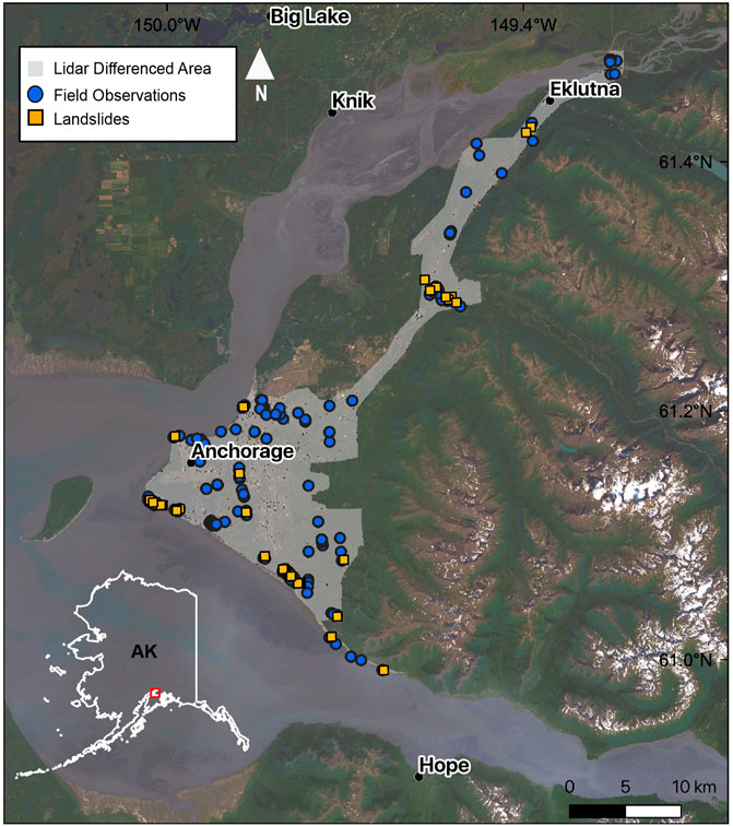
FIGURE 1. Location of the study area within Anchorage, AK. The extent of the lidar differenced area is shown in gray. Landslides are shown as orange squares whereas he approximate location of field observations are shown as blue circles. The field observations consist of multiple photos of all types of ground failure (including ground failure as a result of liquefaction) taken from various vantage points (ground, helicopter). Orange squares are locations that are included in the landslide inventory for this study, which also have corresponding field observations in most cases.

TABLE 1

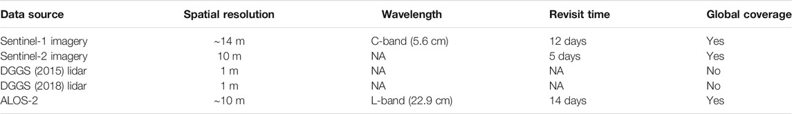
TABLE 1. The spatial resolution, wavelength, revisit time, and coverage offered by the sensors whose data were used in this study.

Using this manually compiled inventory, we then retrospectively evaluate the effectiveness of the three remote sensing methods to identify and delineate the different types of mapped landslides individually without the benefit of manual analysis and combined data sources. We do this by comparing the probability distribution of landslide pixels and the non-landslide pixels for each method. The intention of this exercise is to explore how well these methods might work for automated mapping. Our evaluation methods are detailed in Evaluation of Method Effectiveness.

Field Observations and Optical Imagery

For this study, we used the 1,301 geotagged photos from the ground and helicopter reconnaissance collected by Grant et al. (2020a) within the study area to help map and delineate 43 landslides (Figure 1). Because of the differences in vantage points and cameras used, the accuracy of coordinates associated with each photo varies, thus this field observation database is used primarily with comparisons against high-resolution optical satellite imagery (WorldView-2, WorldView-3, GeoEye-1). We use the high-resolution optical imagery to determine a more accurate location for the manifestations of ground failure in the field photos by matching geographic features seen in the photos to those in the optical imagery (i.e., houses, structures, roads).

Elevation Differencing

Elevation differencing determines the change in elevation between two time periods using digital elevation models (DEMs). The difference in elevation is determined at the pixel scale by subtracting the change in elevation between two aligned pixels (James et al., 2012). This method has proven effective for mapping landslides in a variety of environments and climates (e.g., Bull et al., 2010; Ventura et al., 2011; Prokešová et al., 2014; Mora et al., 2018). The extent of the effectiveness of this method for landslide mapping, however, is dependent on the spatial and temporal resolution of the DEMs, quality of the data, and the extent of coverage.

This study uses 1-m pre- and post-earthquake DEMs derived from lidar data acquired by the state of Alaska and made available via the Alaska Division of Geological and Geophysical Surveys (DGGS) elevation portal (DGGS Staff, 2013). The pre-event data were collected in May 2015 while the post-event data were acquired in December 2018, the week following the earthquake. The reported vertical accuracy for the 2015 DEM is 9.25 cm. Vertical accuracy of the 2018 DEM has not yet been reported by the acquisition team. More information and metadata for these datasets can be downloaded via the DGGS elevation portal (DGGS Staff, 2013). The 2015 DEM was provided in feet, so this raster was converted to meters to remove a vertical offset between the DEMs. The DEMs were aligned by first clipping each to the area of which they both overlap. Then, using the “raster align” tool in QGIS (3.10; https://www.qgis.org/), the clipped DEMs were aligned to one another. Aligning the DEMs involves rescaling and reprojecting the DEMs as needed to ensure that the individual pixels in each image are aligned to one another. After alignment, the DEMs are differenced using the raster calculator in QGIS. The elevation differenced map is computed as

$\text{Elevation}\text{Difference}={\text{DEM}}_{\text{Post}}-{\text{DEM}}_{\text{Pre}}(1)$

in which DEM_Post refers to the 2018 DEM while DEM_Pre refers to the 2015 DEM.

After creating the elevation differenced map, landslides were identified by examining areas within the differenced map that suggested there had been a significant increase or decrease in elevation (relative to surrounding landscape) since the DEM_Pre was acquired (2015). The landslides are visually easy to identify, as most of the study area experienced very little change in elevation. Despite this, a majority of the areas that experienced dramatic changes in elevation since 2015 were related to development and mining activity. Thus, it is necessary to differentiate elevation change that is solely due to landsliding from these other events. To do so, we used high-resolution optical imagery (WorldView-2, WorldView-3, GeoEye-1) to rule out the changes that were the result of development or mining activity.

Normalized Difference Vegetation Index Differencing

NDVI is used to map the relative distribution of vegetation in landscapes. This can be useful for landslide mapping because slope failure often results in damage to vegetation. NDVI maps are generated using the near-infrared (NIR) and red (R) image bands contained within a multispectral image (Deering and Haas, 1980):

$\text{NDVI}=\frac{\text{NIR}-\text{R}}{\text{NIR}+\text{R}}(2)$

Because vegetation absorbs visible light and reflects near-infrared light, this index gives an indication of the health of existing vegetation at the pixel scale. It also maps the relative distribution of vegetation in a landscape because non-vegetated areas are classified with a lower NDVI value. Thus, NDVI differencing maps can reveal areas where vegetation has been damaged or stripped away from the landscape (i.e., due to landslides). Differencing maps can be generated by subtracting the pre-event NDVI pixels from the post-event NDVI pixels. Then, within the change detection image, those pixels that correspond to large changes in NDVI can be further assessed visually to determine whether the change corresponds to a landslide. As previously mentioned, we use optical imagery (WorldView-2, WorldView-3, GeoEye-1) to determine if the NDVI change corresponds to other phenomena such as urban development and/or mining activity.

The lack of sunlight and presence of snow prohibited the creation of accurate NDVI maps in the days immediately preceding and following the event, so we instead used summer NDVI composites from 2018 to 2019 to generate a NDVI differencing map spanning the time of the earthquake. The summer composites were produced using Google Earth Engine (Gorelick et al., 2017) using satellite imagery from the European Space Agency’s Sentinel-2 multispectral satellite. The 10 m resolution composites are generated by taking the median value of each pixel within an image collection after filtering out pixels containing clouds. The composites are then used to produce NDVI maps for the summers preceding and following the earthquake and then differenced to isolate areas where landslides triggered by the earthquake may have caused damage to the normal vegetative cover. The NDVI differenced map is computed as

$\text{NDVI}\text{Difference}={\text{NDVIComp}}_{\text{Pre}}-{\text{NDVIComp}}_{\text{Post}}(3)$

in which NDVIComp_post refers to the summer 2019 NDVI composite and NDVIComp_Pre refers to the summer 2018 NDVI composite.

Synthetic Aperture Radar Amplitude Change Detection

Synthetic aperture radar (SAR) amplitude images measure the proportion of microwave backscattered from that area on the ground, which depends on a variety of factors such as the type, size, shape, orientation, roughness, moisture content, and dielectric constant of reflectors within a given pixel. SAR amplitude change detection (ACD) compares the amplitude intensities between two dates to detect changes in amplitude intensity that may indicate surface changes (e.g., floods, mass movements, or liquefaction events).

Three sets of images are used for change detection before and after the earthquake from the Sentinel-1 and ALOS-2 satellites (Supplementary Table S1). Scene pairs include ascending Sentinel-1 on November 17, 2018 and January 26, 2019, descending Sentinel-1 data on November 22, 2018 and December 4, 2018, and ascending ALOS-2 data on November 17, 2018 and January 26, 2018. Images were processed using SNAP 7.0 software (SNAP - ESA Sentinel Application Platform v7.10, http://step.esa.int). Both Sentinel and ALOS-2 products were radiometrically calibrated to radar reflectivity per unit area, filtered for speckle using a Lee filter operating as a 3 × 3 pixel moving window, corrected for geometric/terrain distortions using a range doppler orthorectification, and composited to determine amplitude changes between the pre-event and post-event image. Pixel intensity was converted to the backscattering coefficient measured in decibel (dB) units that ranges from c. +10 dB for very bright objects to −40 dB for very dark surfaces. Differencing these data that are converted to decibel units is equivalent to the log-ratio method used in other studies (Mondini et al., 2019; Jung and Yun, 2020; Lin et al., 2021) to determine the change in amplitude between SAR scenes. These studies compute the log-ratio value as

${\text{A}}_{\text{ratio}}={\text{log}}_{10}\left(\frac{{\mathrm{A}}_{\text{pre}}}{{\mathrm{A}}_{\text{post}}}\right)(4)$

in which the A_pre and A_post values correspond to the radar brightness coefficient values (Mondini et al., 2019; Jung and Yun, 2020; Lin et al., 2021). Once we converted our data to dB units, the images were then simply differenced as

$\text{Amplitude}\text{Difference}={\text{Amp}}_{\text{Pre}}-{\text{Amp}}_{\text{Post}}(5)$

Additionally, an amplitude change detection time series of Sentinel-1 images between 2015/11/29 and 2020/11/01 was generated using Google Earth Engine (see Data Availability Statement). This approach produces pre- and post-event time series maps utilizing Sentinel-1 ground range detected (GRD) products. GRD products are processed to remove thermal noise and are radiometrically and terrain calibrated. The processed data are also provided in dB units, so the composited time-series maps are differenced as

$\text{Amplitude}\text{Difference}={\text{AmpComp}}_{\text{Pre}}-{\text{AmpComp}}_{\text{Post}}(6)$

In the workflow, image composites are generated for time periods preceding and following the event of interest utilizing VH (vertical transmit, horizontal receive) polarization images. The method utilizes both ascending and descending data to generate the composites. Different polarizations and seasonal composites (i.e., summer months only) did not impact the results. List of the SAR scenes used can be found in the Supplementary Data Sheet S1.

Evaluation of Method Effectiveness

Manual mappers visually look for discontinuities in remote sensing products that correspond to landslides. They typically use knowledge of where landslides are more likely to occur (e.g., steep coastal bluffs, riverbanks) to guide their efforts. Automatic mapping relies on a similar approach and can be implemented using either pixel-based or object-based image analysis methods. Pixel-based methods are those that classify imagery at the pixel scale and do not take into consideration neighboring pixels (Scaioni et al., 2014). Object-based image analysis typically involves the use of thresholding and segmentation techniques (Martha et al., 2011). Thresholding typically entails removing or masking the areas within target images where landslides are least likely to occur, similar to the way in which a manual mapper uses their knowledge of landslide susceptibility to guide their efforts. Segmentation groups the portions of the image into objects comprising similar pixels (Hölbling et al., 2015) working the same way as a human would to identify continuous sets of pixels that may correspond to a landslide. A set of rules, which can be prescribed by the mapper or determined using machine learning algorithms, can be applied to the target image to determine which of the objects or pixel clusters correspond to landslides. Automatic methods tend to struggle with differentiating similar objects from one another, resulting in a large number of false positives (Li et al., 2014). Because of this, automatic methods tend to be more successful when those landslide pixels and subsequently the objects to which they correspond are markedly different from the surrounding pixels (Rosin and Hervas, 2005).

With these concepts in mind, the performance of each of the three remote sensing methods is compared using the probability distributions of landslide pixels versus landscape pixels for each method. This is done in order to determine which methods would be more useful at delineating landslides of different types in this environment using both manual and automatic mapping methods without prior knowledge of the exact location of the landslides. Those landslide pixels that are markedly different from the remaining pixels in the target image would have a probability distribution that differs from the general landscape distribution and thus, likely be more easily identifiable using both manual and automatic approaches.

To generate the probability distributions for each method, we sampled the landslide pixels and landscape pixels of each corresponding raster. We sampled the values at all landslide pixels and then randomly sampled an equal number of pixels from the landscape (non-landslide areas). We then plotted the probability distributions of the sampled landslide and landscape pixels for each method to facilitate comparison. To determine the effect of noise removal on the distributions and to smooth all layers to roughly the same resolution for more direct comparison, the elevation and NDVI differenced raster images were smoothed using a Gaussian filter with a standard deviation of ∼15 m. The results of this smoothing on the distributions can be seen in Supplementary Figure S2. Noise removal did not significantly impact the results, so we do not filter the final data. We show the percentage of observed landslide pixels as a point over each bin in the probability distributions for each method. This displays, for each method, the range of values where landslides are likely to be found.

Landslide Detection and Method Effectiveness

Landslide Inventory

Within the study area, we were able to successfully document the location of 43 landslides using the combined methodologies, including three soil block slides, nine soil slumps, 20 soil slides, nine rapid soil flows, and two rock falls (those landslides that were not classified by those who gathered field observations were classified using the field photos and remote sensing data). Of these landslides, we were able to delineate 39 (90%) as they were easy to identify visually using the remotely sensed data; the remaining 4 (9%) were mapped with a point at the approximate location that was determined using field observations. Field photos of these undelineated landslides (two soil slides and two incipient soil slumps) can be seen in Figure 2. Of the 43 landslide events, 38 (88%) were identifiable using the elevation differenced map and 21 landslides (48%) were identifiable using the NDVI differenced map. No landslides could be delineated using the ACD methods. Remote mapping methods failed to aid in the identification and delineation of four landslides identified in the field, and five landslides not observed in the field were mapped using remote mapping methods. A visual representation of each method is presented in Figure 3. Because the data we used have varying degrees of spatial and temporal resolution, the accuracy of each mapped landslide varies. Accuracy refers to the location of the landslide, the existence of the landslide (i.e., whether it can be confidently attributed to the earthquake) and the delineation. Mapping uncertainty associated with each feature can be found in Supplementary Table S3.

FIGURE 2

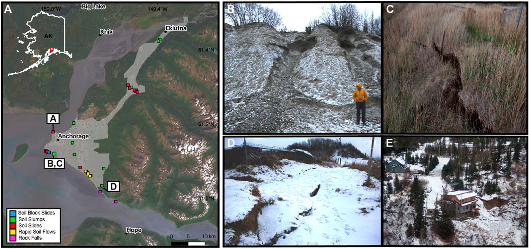
FIGURE 2. The map on the left (A) shows the location of landslides by type as well as the location of those landslides that could not be delineated using remote sensing mapping methods (labeled B–E on the map). Corresponding photos of those landslides can be seen to the right of the map. The top center photo shows a (B) soil slide with a person for scale. The top right (C) and bottom center (D) show incipient soil slumps and the bottom right (E) shows a soil slide. (Photo Credits: USGS).

FIGURE 3

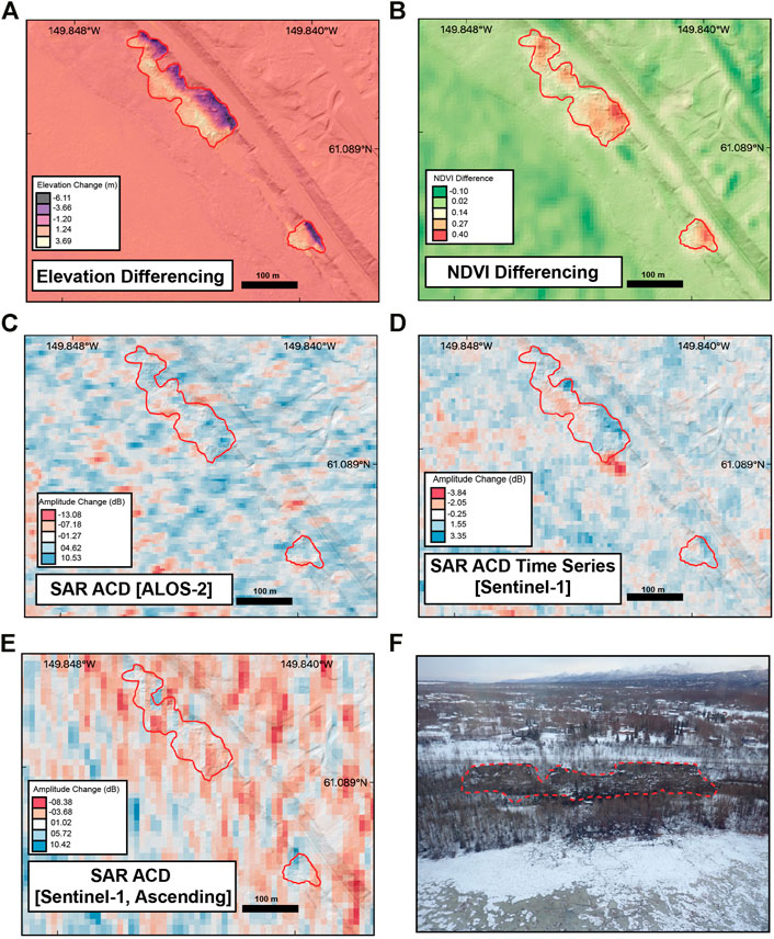
FIGURE 3. An example of the performance of each method at detecting rapid soil flows (outlined in red). Panel (A) shows the performance of elevation differencing and (B) shows the performance of NDVI differencing. Panels C–E display the performance of the remaining SAR ACD methods. An aerial photo of these rapid soil flows can be seen in panel (F) (Photo Credit: USGS).

Method Performance Summary

As previously mentioned, elevation and NDVI differencing were able to aid in the identification and delineation of most landslides whereas ACD methods were largely ineffective. This statement is supported by Figures 4A,B, where the probability distributions of the landslide pixels in the elevation and NDVI change maps differ greatly from those of the remaining landscape in comparison to results from the amplitude-based methods (Figures 4C–F) which are essentially indistinguishable. The distributions of the landscape and landslide pixels for the ACD methods are similar, which suggest that the data are generally too noisy to identify and delineate landslides.

FIGURE 4

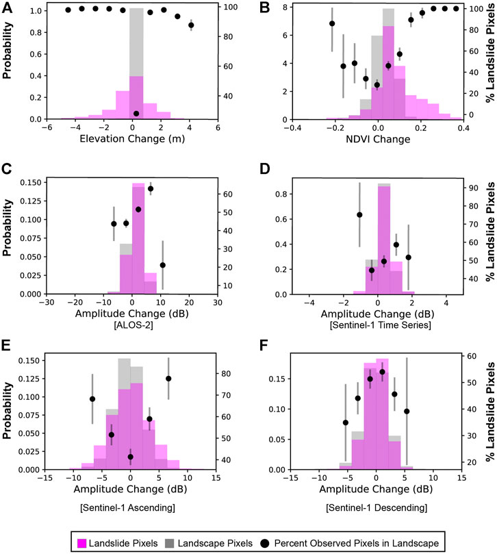
FIGURE 4. Probability distributions comparing landslide pixels to landscape pixels for each method. Panel (A) and (B) display the distributions for the elevation and NDVI differencing, respectively. Panels (C–F) display the distributions of the remaining SAR ACD methods. Confidence interval for each point shown as gray line (significance level 0.05).

For the elevation differenced map, the probability distribution for the landslide pixels is negatively skewed. Because a negative change in elevation corresponds to erosion, this suggests that the landslides mapped are mostly erosional (i.e., soil slides, rapid soil flows). The NDVI change distribution is positively skewed, suggesting that the mapped landslides are those that are severe because they remove vegetation and leave a significant scar on the landscape. The minimum landslide area mapped using elevation differencing was 26 m² while the minimum area mapped by the NDVI differencing method was 355 m². SAR ACD methods were ineffective primarily due to noise (possibly caused by atmospheric interference, snowfall, moisture, and dense vegetation) hindering the delineation and identification of landslides. Additionally, the amplitude values of the resulting landslide scar or deposit were similar to the original landscape (i.e., soil slide occurring in areas of unvegetated, exposed soil), preventing the utility of this method. Geometric distortion also prevented any delineation of landslides along coastal bluffs using the SAR ACD methods. Because of these issues with SAR ACD methods, we will only discuss the effectiveness of elevation and NDVI differencing to delineate landslide types in subsequent sections.

Elevation Differencing

The probability distributions for the soil slumps, soil slides, and rapid soil flows suggest that elevation differencing was more effective at delineating these landslide types than the others (soil block slides and rock falls) in our study area (Figures 5C, E, G). This is based on the fact that the distribution of landslide pixels for these landslide types differs from the general landscape distribution and also because, over a certain range of elevation change values, a relatively high percentage of landslide pixels is observed. Landslide pixels associated with soil block slides and rock falls (Figures 5A,I) are too similar to the remaining landscape distribution to state that elevation differencing can be effective at delineating those landslide types automatically. Despite this, the field observations allowed us to identify and delineate the soil block slides using the elevation differenced map. So, in regard to manual mapping, the differencing was helpful to delineate these types of landslides but only with prior knowledge of likely landslide locations. This suggests that automatic methods may not be able to systematically map soil block slides using elevation differencing. Rock falls, in our study area, were not able to be delineated using the lidar differenced map. Even with knowledge that they occurred and the general vicinity in which they occurred, delineation was challenging. This could be attributed to their deposits being thin and the time difference between the lidar datasets producing noise that corresponds to non-earthquake related changes. Only two rock falls were mapped in the study area, which limits our observations of these features.

FIGURE 5

FIGURE 5. Probability distributions comparing landslide pixels to landscape pixels by landslide type for the elevation and NDVI differencing methods. Panels (A) and (B) display the distributions that correspond to soil block slides for the elevation and NDVI differencing methods, respectively. Similarly, panels (C) and (D) correspond to soil slumps, panels (E) and (F) correspond to soil slides, (G)and (H) correspond to rapid soil flows and (I) and (J) correspond to rock falls. Confidence interval for each point shown as gray line (significance level 0.05).

Normalized Difference Vegetation Index Differencing

The probability distributions for the soil slumps and rapid soil flows suggest that NDVI differencing was more effective at delineating these landslide types than the others (Figures 5D,H). This is based on the fact that the distribution of landslide pixels for these landslide types differs from the general landscape distribution and also because, over a certain range of NDVI change values a relatively high percentage of landslide pixels is observed. Soil block slides, soil slides, and rock falls (Figures 5B, F, J) are too similar to the remaining landscape distribution to state that NDVI differencing is effective at delineating these landslide types.

Discussion

In this study, lidar elevation differencing and NDVI differencing are proven to be more effective at identifying and delineating landslides in an urban subarctic environment than SAR ACD methods. Elevation differencing proved useful to identify and delineate soil slumps, soil slides and rapid soil flows, while NDVI differencing is more effective at capturing soil slumps and rapid soil flows. The success of the elevation differencing method at delineating soil slumps, soil slides and rapid soil flows can be attributed to the fact that they have distinct erosional or depositional signatures which increases the extent of the landslide affected area. Because soil slumps tend to result in a large, semi-coherent landslide deposit left in the landscape, the probability distribution for this landslide type is positively skewed and thus, these landslides are easy to delineate using elevation differenced data. Soil slides and rapid soil flows have an elongated erosional signature with small and thin deposits, which result in a negatively skewed probability distribution.

The success of the NDVI differencing method at delineating soil slumps and rapid soil flows can be attributed to their severity and size, with the major limiting factor being that landslides need to occur in vegetated areas in order for NDVI methods to be useful. Because soil slumps and rapid soil flows are disruptive to the overlying vegetation, they have the potential to have a lasting impact on the landslide affected area. Even though the images used in our study are a year apart, these landslides are still able to be delineated due to their severity and ability to leave a lasting scar on the landscape. Thus, in scenarios where these landslide types are known to have been triggered, the methods presented here could prove useful at identifying those landslides and delineating them.

Although the earthquake occurred in late fall with winter conditions, seasonal NDVI composites preceding and following the earthquake were shown to be effective at identifying and delineating landslides. Because the NDVI composites were generated using widely available Sentinel-2 data, the method can be easily implemented in future studies. The resolution of this data (10 m resolution), however, may fail to map smaller landslides. In this study, for instance, the minimum landslide area that could be mapped using the NDVI differenced data was 355 m². While not widely available, higher resolution imagery containing NIR bands, such as from the WorldView sensors, may be able to generate higher resolution NDVI differencing maps.

Challenges to Overcome

While we were able to effectively identify and delineate landslides observed in the field using the remote sensing methods, and delineate an additional five that were not identified in the field, we also faced many challenges that prevented us from mapping all landslides in our study area. Snow accumulation and lack of sunlight were the primary challenges associated with landslide mapping using field and multispectral data, but the expression of the landslides due to the nature of the ground motion also played a crucial role. Despite the November 30 earthquake being the largest earthquake since the M 9.2 Great Alaska earthquake to affect the Anchorage area, the landslides triggered were generally small, shallow, and limited in number (Jibson et al., 2020). Many slope failures consisted of minor slope cracking and deformation (e.g., Figure 2) that may result in costly damage to structures but are too subtle to identify via the remote sensing methods. In addition, many of these geotechnical failures were repaired prior to the date of the post-event imagery used in this study (we had to wait until the Spring or Summer for post-event images to be of sufficient quality for mapping). To summarize, producing a complete and high-quality landslide inventory is challenging for this particular earthquake due to the environmental conditions as well as the subdued surface expression of the landslides.

Within our study area, we failed to delineate soil slides and soil slumps that were identified in the field with remotely sensed data. This is primarily attributed to the resolution of the NDVI (∼10 m) and elevation data (1 m) because these failures were small. This may also result in a failure to effectively map rock falls as well. However, there were only two rock falls in our study area so with this small sample size it is difficult to definitively say if rock falls are generally challenging to map using the methods presented here. Additionally, NDVI may have failed to capture some landslides due to the composites being produced from images taken several months before and after the earthquake event, if vegetation disruption was minor, the vegetative cover could have fully recovered in that time. While we were able to successfully use NDVI differencing to map other landslides in our study area, this method is unfortunately not applicable above tree line in arid or semi-arid environments due to a lack of vegetation and thus lack of changes in vegetation due to landslide scouring. Though outside the study area, there were some rock falls above tree line in the mountainous areas east of Anchorage (Grant et al., 2020b; Jibson et al., 2020). Elevation differencing can solve these issues, however there are limitations related to data availability as well as the spatial and temporal resolution of the data. Here, our mapping was limited by the extent of the 1-m DEM data and the 3-year time difference between the pre- and post-DEMs. One way to overcome this may be to use the DEMs available as part of the ArcticDEM project (Porter et al., 2018). The ArcticDEM data are derived from stereo satellite imagery and made available for a large portion of the northern latitudes at 2 m resolution. The data are periodically released, however, and at the time of publication the latest release did not include any post-earthquake DEMs. Depending on data access and computer processing power, one could also generate these DEMs using stereo satellite imagery and the NASA AMES stereo pipeline (Beyer et al., 2018). One limitation, however, is that unlike lidar methods, the ArcticDEM project produces a digital surface model (DSM) that does not remove vegetation. This emphasizes the importance of collecting regular “pre-event” baseline data to facilitate rapid and reliable mapping.

Despite the many advantages of using SAR sensors for mapping surface changes, SAR ACD methods were not effective at mapping landslides in this study due to several geomorphologic, radiometric, and image processing factors (see Mondini et al., 2021 for a recent review). During image pre-processing, both horizontal-horizontal (HH) and horizontal-vertical (HV) polarization scenes were considered. HV scenes typically had lower (darker) backscatter and did not improve landslide detection, therefore only HH scene results are shown herein. Additionally, we found that a Lee filter operating as a 3 × 3 pixel moving window sufficiently reduced speckle, as determined visually and by comparing the variance in the intensity image before and after filtering.

Multiple platforms with different SAR bands and look directions were used to optimize landslide detection. A direct comparison of C-band (Sentinel-1) versus L-band (ALOS-2) performance is challenging due to the different temporal and spatial resolutions of the scenes. While the L-band scene contained less speckle than the C-band scenes, it did not result in an improvement in landslide detection. Landslide events must cause surface changes of a significant magnitude to be recognizable in the SAR imagery, thus changes in the amplitude were not sufficiently higher than the noise or speckle effect to identify surface changes. One of the most significant limiting factors for landslide detection in this study was illumination issues caused by the side-looking geometry of the SAR system, which results in geometric distortions in steep terrain, such as layover (top of a backscattering object is recorded closer to the radar than the lower parts of the objects) and radar shadows (lack of radar illumination). While both ascending and descending scenes were considered, steep, south-facing slopes where many of the landslides occurred still experienced significant geometric distortions, preventing landslide detection.

SAR can penetrate clouds and image during the day or a night, providing a potential workaround for mapping in the dark in subarctic and arctic regions. However, the snow coverage may have resulted in the large amount of noise present in our SAR scenes. Thus, the main question arising from this work is what other methods can we further develop to help with landslide mapping in dark, snow covered environments? A second questions is: what methods will help to map small and subdued landslides? The motivation for the first question is due to the need for mapping in subarctic regions, the second question arises from the fact that in many instances’ landslide inventories are produced for events that are extreme and leave an easily discernible mark on the landscape (Tanyaş et al., 2018). Thus, the landslide inventories that are generally used for modeling efforts tend to rely on information from these dramatic events and not events that result in smaller landslides. This situation results in subsequent models relying on these inventories to be biased. The answer to both questions can be obtained by further testing and developing methods in such an environment (where visibility is limited due to snow and lack of sunlight) and under similar conditions (limited surface expression of landslide damage).

Our work indicates the value of closely analyzing and further developing remote mapping methods in environments such as Anchorage, AK, and for events that result in minor surface deformation. A similar earthquake event occurred on March 31, 2020, in Stanley, Idaho. After the M_w 6.5 earthquake, USGS field reconnaissance efforts were restricted due to the ongoing COVID-19 pandemic. In addition, local response was stymied due to avalanche risk and late season snow limiting ground visibility via aircraft (Idaho Geological Survey, 2020). The Idaho event is just one example that highlights the utility of remote mapping in an environment such as Anchorage, AK. Anthropogenic climate change has also been shown to alter the characterization and frequency of landslides occurring in subarctic conditions (Coe et al., 2018; Coe, 2020) suggesting that developing such methods will be of high importance into the future. Here, we suggest that exploring remote mapping methods systematically can lead to a better understanding of landslide mapping in such an environment. Such development in the field could then greatly improve earthquake-triggered landslide susceptibility and hazard models.

The challenges left to overcome relate mainly to the resolution and quality of the data available. ArcticDEM data could potentially be used to map landslides in subarctic environments. Additionally, higher resolution satellite imagery could be used to generate NDVI maps. Digital image correlation (DIC) of high-resolution satellite imagery may be more effective at capturing coherent landslides such as soil block slides (Bickel et al., 2018). Despite the ineffectiveness of the SAR ACD methods, InSAR (Interferometric Synthetic Aperture Radar) could be used to map coherent deformation, such as lateral spreading, as well (Saroli et al., 2005). The NASA-ISRO SAR mission (NISAR) with a projected launch date of 2022, will have a long (L-band) wavelength, 3–10 m resolution, temporal resolution of 12 days, and will be freely available and open to the public. Since L-band radar can penetrate the tree canopy at greater depths than C-band, these new data may be useful in detecting landslides in forested areas (Rosen et al., 2017).

Conclusion

In our study, we provide evidence that remote mapping can augment field-based inventories by aiding in the discovery of previously unobserved landslides and also help to better delineate the landslide-affected area. Simultaneously, we also highlight the importance of rapid post-earthquake field observations in environments such as Anchorage, AK, as these allowed us to build an adequate inventory and also develop methods to map the remaining area affected by the earthquake.

Broadly, we demonstrate a gap in our knowledge of earthquake-triggered ground failure in arctic and subarctic environments in winter conditions because of difficulties in remote mapping under such circumstances. With many earthquake-prone areas subject to such circumstances (northern Japan, Alaska, Canada, Iceland) and many other regions prone to similar geologic conditions and winter weather, there is merit in determining an effective way to map landslides in such an environment. To date, few earthquake-induced landslide inventories are located in these subarctic environments despite the relatively high amount of seismic activity (Tanyaş et al., 2018). Many of the identified challenges are not unique to Alaska; thus, the observations and mapping methods described in this study can provide the foundation for others to develop workflows for mapping landslides in subarctic and urban regions and improve response and landslide inventory efforts in these challenging environments.

Data Availability Statement

Snowfall data were accessed using the Interactive Snow Information website maintained by the National Operational Hydrologic Remote Sensing Center (https://www.nohrsc.noaa.gov/interactive). High-resolution satellite imagery was downloaded using the MAXAR Global Enhanced GEOINT Delivery (G-EGD) system. The Google Earth Engine code used to create the synthetic aperture radar (SAR) amplitude change detection (ACD) time series maps can be accessed via GitHub at the following link: https://github.com/MongHanHuang/GEE_SAR_landslide_detection(https://doi.org/10.5281/zenodo.4060268). The landslide inventory used in our analysis is provided by Martinez et al. (2021). Field observation data can be found in Grant et al. (2020a).

Author Contributions

The study was conceived by KEA, EMT, LNS, and SNM. Field inventory and landslide inventory were created by SNM. Elevation, NDVI differencing, and SAR ACD time series maps were derived by SNM. ALOS-2 and Sentinel-1 SAR ACD maps were derived by LNS. Probability distribution analysis was carried out by SNM. KEA and EMT guided the structure of the work. All authors contributed to discussion of findings and implications for future work.

Conflict of Interest

The authors declare that the research was conducted in the absence of any commercial or financial relationships that could be construed as a potential conflict of interest.

Disclaimer

Any use of trade, firm, or product names is for descriptive purposes only and does not imply endorsement by the U.S. Government.

Acknowledgments

We would like to acknowledge Rob Witter, Alex Grant, and Randall W. Jibson (U.S. Geological Survey) for their constructive feedback throughout the duration of this project as well as for their contributions to the field observations database. We would also like to thank Barrett Salisbury from the Alaska Department of Natural Resources (Alaska DNR) for his support in regard to data accessibility and information regarding the earthquake event. Thank you to Stephen Slaughter and Jeffrey Coe (U.S. Geological Survey) for their helpful suggestions and comments. And lastly, thank you to the reviewers for their careful review and constructive feedback.

Supplementary Material

The Supplementary Material for this article can be found online at: https://www.frontiersin.org/articles/10.3389/feart.2021.673137/full#supplementary-material

References

Baum, R. L., Godt, J. W., and Savage, W. Z. (2010). Estimating the Timing and Location of Shallow Rainfall-Induced Landslides Using a Model for Transient, Unsaturated Infiltration. J. Geophys. Res. Earth Surf. 115, 1–26. doi:10.1029/2009jf001321

CrossRef Full Text | Google Scholar

Beyer, R. A., Alexandrov, O., and McMichael, S. (2018). The Ames Stereo Pipeline: NASA’s Open Source Software for Deriving and Processing Terrain Data. Earth Space Sci. 5, 537–548. doi:10.1029/2018ea000409

CrossRef Full Text | Google Scholar

Bickel, V., Manconi, A., and Amann, F. (2018). Quantitative Assessment of Digital Image Correlation Methods to Detect and Monitor Surface Displacements of Large Slope Instabilities. Remote Sens. 10 (6), 865. doi:10.3390/rs10060865

CrossRef Full Text | Google Scholar

Booth, A. M., Roering, J. J., and Perron, J. T. (2009). Automated Landslide Mapping Using Spectral Analysis and High-Resolution Topographic Data: Puget Sound Lowlands, Washington, and Portland Hills, Oregon. Geomorphology 109 (3–4), 132–147. doi:10.1016/j.geomorph.2009.02.027

CrossRef Full Text | Google Scholar

Bull, J. M., Miller, H., Gravley, D. M., Costello, D., Hikuroa, D. C. H., and Dix, J. K. (2010). Assessing Debris Flows Using LIDAR Differencing: 18 May 2005 Matata Event, New Zealand. Geomorphology 124, 75–84. doi:10.1016/j.geomorph.2010.08.011

CrossRef Full Text | Google Scholar

Coe, J. A. (2020). Bellwether Sites for Evaluating Changes in Landslide Frequency and Magnitude in Cryospheric Mountainous Terrain: A Call for Systematic, Long-Term Observations to Decipher the Impact of Climate Change. Landslides 17, 2483–2501. doi:10.1007/s10346-020-01462-y

CrossRef Full Text | Google Scholar

Coe, J. A., Bessette-Kirton, E. K., and Geertsema, M. (2018). Increasing Rock-Avalanche Size and Mobility in Glacier Bay National Park and Preserve, Alaska Detected From 1984 to 2016 Landsat Imagery. Landslides 15, 393–407. doi:10.1007/s10346-017-0879-7

CrossRef Full Text | Google Scholar

Colesanti, C., and Wasowski, J. (2006). Investigating Landslides With Space-Borne Synthetic Aperture Radar (SAR) Interferometry. Eng. Geol. 88, 173–199. doi:10.1016/j.enggeo.2006.09.013

CrossRef Full Text | Google Scholar

Deering, D. W., and Haas, R. H. (1980). Using Landsat Digital Data for Estimating Green Biomass. NASA Tech. Memo. 80727, 1.

Google Scholar

DGGS Staff (2013). Elevation Datasets of Alaska: Alaska Division of Geological & Geophysical Surveys Digital Data Series 4. Available at: https://maps.dggs.alaska.gov/elevationdata/ (Accessed June 1, 2020).

Google Scholar

Franke, K. W., Koehler, R. D., Beyzaei, C. Z., Cabas, A., Pierce, I., Stuedlein, A., et al. (2019). Geotechnical Engineering Reconnaissance of the 30 November 2018 Mw 7.0 Anchorage, Alaska Earthquake. GEER Report GEER-059, 1–46. (Accessed June 1, 2020).

Google Scholar

Galli, M., Ardizzone, F., Cardinali, M., Guzzetti, F., and Reichenbach, P. (2008). Comparing Landslide Inventory Maps. Geomorphology 94, 268–289. doi:10.1016/j.geomorph.2006.09.023

CrossRef Full Text | Google Scholar

Gorelick, N., Hancher, M., Dixon, M., Ilyushchenko, S., Thau, D., and Moore, R. (2017). Google Earth Engine: Planetary-Scale Geospatial Analysis for Everyone. Remote Sens. Environ. 202, 18–27. doi:10.1016/j.rse.2017.06.031

CrossRef Full Text | Google Scholar

Grant, A. R., Jibson, R. W., Witter, R. C., Allstadt, K., Thompson, E., Bender, A. M., et al. (2020a). Field Reconnaissance of Ground Failure Triggered by Shaking During the 2018 M7.1 Anchorage, Alaska, Earthquake: U.S. Geological Survey Data Release. Open-File Report 2020-1043. (Accessed June 1, 2020).

Google Scholar

Grant, A. R. R., Jibson, R. W., Witter, R. C., Allstadt, K. E., Thompson, E. M., and Bender, A. M. (2020b). Ground Failure Triggered by Shaking during the November 30, 2018, Magnitude 7.1 Anchorage, Alaska, Earthquake: U.S. Geological Survey. Open-File Report 2020-1043. (Accessed June 1, 2020).

Google Scholar

Guzzetti, F., Mondini, A. C., Cardinali, M., Fiorucci, F., Santangelo, M., and Chang, K.-T. (2012). Landslide Inventory Maps: New Tools for an Old Problem. Earth-Sci. Rev. 112, 42–66. doi:10.1016/j.earscirev.2012.02.001

CrossRef Full Text | Google Scholar

Hansen, W. R. (1965). Effects of the Earthquake of March 27, 1964, at Anchorage, Alaska. Washington, DC. US Government Printing Office.

Google Scholar

Harp, E. L., Jibson, R. W., and Schmitt, R. G. (2016). Map of Landslides Triggered by the January 12, 2010, Haiti Earthquake: Scientific Investigations Map Reston, VA. U.S. Geological Survey, 15.

Google Scholar

Hölbling, D., Friedl, B., and Eisank, C. (2015). An Object-Based Approach for Semi-Automated Landslide Change Detection and Attribution of Changes to Landslide Classes in Northern Taiwan. Earth Sci. Inform. 8, 327–335. doi:10.1007/s12145-015-0217-3

CrossRef Full Text | Google Scholar

Idaho Geological Survey (2020). M6.5 Stanley, ID Earthquake Aerial Reconnaissance Report. Available at: https://www.idahogeology.org/pub/Other/IGS_Stanley_EQ_Recon_Summary_20200406.pdf. (Accessed June 1, 2020).

Google Scholar

James, L. A., Hodgson, M. E., Ghoshal, S., and Latiolais, M. M. (2012). Geomorphic Change Detection Using Historic Maps and DEM Differencing: The Temporal Dimension of Geospatial Analysis. Geomorphology 137, 181–198. doi:10.1016/j.geomorph.2010.10.039

CrossRef Full Text | Google Scholar

Jibson, R. W., R. Grant, A. R., Witter, R. C., Allstadt, K. E., Thompson, E. M., and Bender, A. M. (2020). Ground Failure From the Anchorage, Alaska, Earthquake of 30 November 2018. Seismol. Res. Lett. 91 (1), 19–32. doi:10.1785/0220190187

CrossRef Full Text | Google Scholar

Jung, J., and Yun, S.-H. (2020). Evaluation of Coherent and Incoherent Landslide Detection Methods Based on Synthetic Aperture Radar for Rapid Response: A Case Study for the 2018 Hokkaido Landslides. Remote Sens. 12 (2), 265. doi:10.3390/rs12020265

CrossRef Full Text | Google Scholar

Keefer, D. K. (1984). Landslides Caused by Earthquakes. Geol. Soc. Am. Bull. 95, 406–421. doi:10.1130/0016-7606(1984)95<406:lcbe>2.0.co;2

CrossRef Full Text | Google Scholar

Larsen, I. J., and Montgomery, D. R. (2012). Landslide Erosion Coupled to Tectonics and River Incision. Nat. Geosci. 5, 468–473. doi:10.1038/ngeo1479

CrossRef Full Text | Google Scholar

Li, G., West, A. J., Densmore, A. L., Jin, Z., Parker, R. N., and Hilton, R. G. (2014). Seismic Mountain Building: Landslides Associated with the 2008 Wenchuan Earthquake in the Context of a Generalized Model for Earthquake Volume Balance. Geochem. Geophys. Geosyst. 15, 833–844. doi:10.1002/2013gc005067

CrossRef Full Text | Google Scholar

Lin, S.-Y., Lin, C.-W., and Van Gasselt, S. (2021). Processing Framework for Landslide Detection Based on Synthetic Aperture Radar (SAR) Intensity-Image Analysis. Remote Sens. 13 (4), 644. doi:10.3390/rs13040644

CrossRef Full Text | Google Scholar

Martha, T. R., Kerle, N., van Westen, C. J., Jetten, V., and Kumar, K. V. (2011). Segment Optimization and Data-Driven Thresholding for Knowledge-Based Landslide Detection by Object-Based Image Analysis. IEEE Trans. Geosci. Remote Sens. 49, 4928–4943. doi:10.1109/tgrs.2011.2151866

CrossRef Full Text | Google Scholar

Martinez, S. N., Schaefer, L. N., Allstadt, K. E., and Thompson, E. M. (2021). Initial Observations of Landslides Triggered by the 2018 Anchorage, Alaska Earthquake. USGS Data Release (Accessed June 1, 2020).

Google Scholar

Mirus, B. B., Becker, R. E., Baum, R. L., and Smith, J. B. (2018). Integrating Real-Time Subsurface Hydrologic Monitoring with Empirical Rainfall Thresholds to Improve Landslide Early Warning. Landslides 15, 1909–1919. doi:10.1007/s10346-018-0995-z

CrossRef Full Text | Google Scholar

Mirus, B. B., Jones, E. S., Baum, R. L., Godt, J. W., Slaughter, S., Crawford, M. M., et al. (2020). Landslides Across the USA: Occurrence, Susceptibility, and Data Limitations. Landslides 17, 2271–2285. doi:10.1007/s10346-020-01424-4

CrossRef Full Text | Google Scholar

Mondini, A. C., Guzzetti, F., Chang, K. T., Monserrat, O., Martha, T. R., and Manconi, A. (2021). Landslide Failures Detection and Mapping Using Synthetic Aperture Radar: Past, Present and Future. Earth-Sci. Rev. 216, 103574. doi:10.1016/j.earscirev.2021.103574

CrossRef Full Text | Google Scholar

Mondini, A., Santangelo, M., Rocchetti, M., Rossetto, E., Manconi, A., and Monserrat, O. (2019). Sentinel-1 SAR Amplitude Imagery for Rapid Landslide Detection. Remote Sens. 11 (7), 760. doi:10.3390/rs11070760

CrossRef Full Text | Google Scholar

Mora, O., Lenzano, M., Toth, C., Grejner-Brzezinska, D., and Fayne, J. (2018). Landslide Change Detection Based on Multi-Temporal Airborne LiDAR-Derived DEMs. Geosciences 8, 23. doi:10.3390/geosciences8010023

CrossRef Full Text | Google Scholar

Nowicki Jessee, M. A., Hamburger, M. W., Allstadt, K., Wald, D. J., Robeson, S. M., Tanyas, H., et al. (2018). A Global Empirical Model for Near‐Real‐Time Assessment of Seismically Induced Landslides. J. Geophys. Res. Earth Surf. 123, 1835–1859. doi:10.1029/2017jf004494

CrossRef Full Text | Google Scholar

Porter, C., Morin, P., Howat, I., Noh, M.-J., Bates, B., Peterman, K., et al. (2018). ArcticDEM. Harvard Dataverse, V1. https://www.pgc.umn.edu/data/arcticdem/ (Accessed June 1, 2021).

Google Scholar

Prokešová, R., Kardoš, M., Tábořík, P., Medveďová, A., Stacke, V., and Chudý, F. (2014). Kinematic Behaviour of a Large Earthflow Defined by Surface Displacement Monitoring, DEM Differencing, and ERT Imaging. Geomorphology 224, 86–101.

Google Scholar

Rosen, P., Hensley, S., Shaffer, S., Edelstein, W., Kim, Y., Kumar, R., et al. (2017). “The NASA-ISRO SAR (NISAR) Mission Dual-Band Radar Instrument Preliminary Design,” in 2017 IEEE International Geoscience and Remote Sensing Symposium (IGARSS) Fort Worth, TX, July 23–28, 2017, 3832–3835.

Google Scholar

Rosin, P. L., and Hervás, J. (2005). Remote Sensing Image Thresholding Methods for Determining Landslide Activity. Int. J. Remote Sens. 26, 1075–1092. doi:10.1080/01431160512331330481

CrossRef Full Text | Google Scholar

Rott, H., and Nagler, T. (2006). The Contribution of Radar Interferometry to the Assessment of Landslide Hazards. Adv. Space Res. 37, 710–719. doi:10.1016/j.asr.2005.06.059

CrossRef Full Text | Google Scholar

Saroli, M., Stramondo, S., Moro, M., and Doumaz, F. (2005). Movements Detection of Deep Seated Gravitational Slope Deformations by Means of InSAR Data and Photogeological Interpretation: Northern Sicily Case Study. Terra Nova 17 (1), 35–43. doi:10.1111/j.1365-3121.2004.00581.x

CrossRef Full Text | Google Scholar

Scaioni, M., Longoni, L., Melillo, V., and Papini, M. (2014). Remote Sensing for Landslide Investigations: An Overview of Recent Achievements and Perspectives. Remote Sens. 6 (10), 9600–9652. doi:10.3390/rs6109600

CrossRef Full Text | Google Scholar

Stanley, T., and Kirschbaum, D. B. (2017). A Heuristic Approach to Global Landslide Susceptibility Mapping. Nat. Hazards 87, 145–164. doi:10.1007/s11069-017-2757-y

PubMed Abstract | CrossRef Full Text | Google Scholar

Tanyaş, H., Allstadt, K. E., and van Westen, C. J. (2018). An Updated Method for Estimating Landslide-Event Magnitude. Earth Surf. Process. Landf. 43, 1836–1847. doi:10.1002/esp.4359

CrossRef Full Text | Google Scholar

Tanyaş, H., and Lombardo, L. (2020). Completeness Index for Earthquake-Induced Landslide Inventories. Eng. Geol. 264, 105331. doi:10.1016/j.enggeo.2019.105331

CrossRef Full Text | Google Scholar

Tanyaş, H., Van Westen, C. J., Allstadt, K. E., Anna Nowicki Jessee, M., Görüm, T., Jibson, R. W., et al. (2017). Presentation and Analysis of a Worldwide Database of Earthquake-Induced Landslide Inventories. J. Geophys. Res. Earth Surf. 122, 1991–2015. doi:10.1002/2017JF004236

CrossRef Full Text | Google Scholar

Ventura, G., Vilardo, G., Terranova, C., and Sessa, E. B. (2011). Tracking and Evolution of Complex Active Landslides by Multi-Temporal Airborne LiDAR Data: The Montaguto Landslide (Southern Italy). Remote Sens. Environ. 115, 3237–3248. doi:10.1016/j.rse.2011.07.007

CrossRef Full Text | Google Scholar